Article

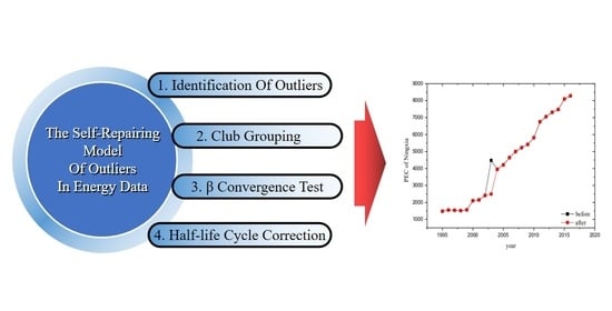
Research on the Self-Repairing Model of Outliers in Energy Data Based on Regional Convergence

1
Key Laboratory of Ocean Energy Utilization and Energy Conservation of Ministry of Education, Dalian University of Technology, Dalian 116024, China
2
School of Economics and Management, China University of Petroleum, Beijing 102249, China
*
Author to whom correspondence should be addressed.
Energies 2020, 13(18), 4909; https://doi.org/10.3390/en13184909
Submission received: 3 August 2020 / Revised: 12 September 2020 / Accepted: 15 September 2020 / Published: 18 September 2020
(This article belongs to the Section C: Energy Economics and Policy)

Abstract

:
The need for the statistical stability of data is increasing nowadays as the data resource has become a more and more important production factor. In this study, a set of general identification and correction models are established for data outlier modification. The research object we chose is the data of per capita energy consumption. Based on the joint diagnosis method of outliers and the regional convergence theory, the abrupt outliers are identified and corrected. The study finds that there is an outlier in the data of the Ningxia Hui Autonomous Region. According to the club grouping method, 30 provinces in China are divided into two clubs and the Ningxia Hui Autonomous Region is determined to be in the first club. We calculate the convergence rate and obtain the correction results combining the half-life cycle model.

Graphical Abstract

1. Introduction

With the rapid development of information technology, the data resource has become an important factor of production, with more attention being paid to its stability. The energy industry is the foundation of national economic and social development, which is also deeply influenced by big data. Energy statistics are the cornerstone of energy research and policymaking. People have been trying to make the energy data as complete as possible, and few attempts have been made to verify and correct abnormal data. In this paper, we utilize regional convergence theory and the half-life cycle model to correct outlier in energy statistic data. For the identification process of outliers, the joint diagnosis method based on the autoregressive moving average (ARMA) model of a time series is used.
The study of regional convergence theory began in the mid-20th century, developed from Solow’s neoclassical growth model [1]. The main idea is that economies tend to develop into the same steady-state from time to time due to the nature of diminishing marginal returns. In the 1980s, the study on convergence began to develop and the types of convergence were divided into four main types: σ convergence, β convergence, γ convergence and club convergence. Baumol (1986) [2] conducted an empirical study on convergence first and showed that the growth rate of productivity in industrialized countries is negatively corrected with its productivity level. Barro and Sala-i-Martin (1991) [3] proposed the econometric definitions of sigma convergence and beta convergence. Sigma convergence refers to the narrowing of the average income gap over time. Beta convergence means the growth rate of per capita income in underdeveloped regions is higher than that in developed regions, which shows a “catch-up effect”. Barro (2003) [4] analyzed panel data of per capita GDP of 100 countries from 1960 to 1990 and verified the existence of conditional convergence. Chambers (2016) [5] constructed the income distribution convergence model of 81 countries from 1990 to 2010 using the Gini coefficient and income mean logarithmic deviation cross-section data and panel data. Leonardo (2018) [6] studied whether the labor productivity of different regions in Peru convergent from 2002 to 2012, the results show that the labor productivity of Peru’s secondary industry (especially manufacturing industry) is convergent, while the labor productivity of agriculture and service industry is not convergent. With regard to the development of regional convergence theory, the research field gradually extended from economics to others, and an increasing amount of papers begin to study the convergence research of energy issues. List (1999) [7] used the time-series analysis method for the first time to study whether the income convergence in the United States is accompanied by the convergence of air pollutant emissions from 1929 to 1994. Mishra (2014) [8] uses panel Kwiatkowski–Phillips–Schmidt–Shin (KPSS) stationarity test and Lagrange multiplier unit root test to verify the convergence of energy consumption per capita in Association of Southeast Asian Nations (ASEAN) countries from 1971 to 2011. Sheng (2014) [9] analyzed the panel data of 27 provinces in China from 1978 to 2008, and used regression to study the relationship between China’s economic growth, energy demand and relevant policies. Apergis (2016) [10] tested the convergence of wholesale electricity prices in big Australian states. Solarin (2018) [11] used a more flexible fractional integrator-based method to test the hypothesis of convergence of renewable energy consumption in 27 Organization for Economic Co-operation and Development (OECD) countries.
In the mid-1990s, with the development of the study on time and space characteristics of the regional economy, club convergence theory began to get more attention. Club convergence refers to the convergence of economic growth of a group of regions in the same initial conditions and structural characteristics of economic growth to the same steady state. Barro and Sala-i-Martin (1991) propose the concept of club convergence, and they regard club convergence as the β convergence of a regional group that has similar initial economic conditions and structural characteristics of economic growth. Galor (1996) [12] argued that the traditional neoclassical growth model gives rise to the club convergence hypothesis and conditional convergence hypothesis, and also proposes the concept of club convergence. Phillips and Sul (2007) [13,14] propose the nonlinear time-varying factor model(log-t), which is an important method of convergence test based on regression. Kim (2012) [15] studied the dynamic behavior of electricity consumption and used the log-t test to conduct club grouping and convergence tests for 109 countries from 1971 to 2009. Paker (2016) [16] analyzed the convergence of global economic and manufacturing energy productivity clubs by taking 33 countries including OECD and non-OECD nations as samples. Based on the log-t method, there are energy productivity clubs and six manufacturing clubs in the global economy. Adrian (2016) [17] tested the homogeneity of 12 tourist source markets in Spain. Cuñado [18,19,20] examined the real convergence hypothesis in some countries by means of using time-series techniques.
The half-life model is established by Art Schneiderman in the United States, and its main content is that the failure rate level presents a negative correlation over a certain period. When giving the defect rate at the initial level and at the lowest level, the time required to reduce the defect rate by half is the half-life cycle. Romer (2001) [21] pointed out that the half-life cycle can be calculated when the convergence rate is known, which is the number of years needed to reduce the national income gap by half. Moon (2017) [22] investigated the half-life cycle of the relative consumer price index in 15 regions of Korea from 1990 to 2016. Bergman (2017) [23] analyzed the half-life circle of 124 homogeneous commodities in Denmark from 1997 to 2010, which was 9.4 months when taking deviation into account, and 28.7 months when adopting the standard method.
The diagnosis of time-series outliers began in the 1970s. Fox (1972) [24] was the first one to define and classify outliers, who took two kinds of outliers into account in the time-series model: additive outliers (AO) that affect only one observation, and innovative outliers (IO) that continuously affect several observations. Tsay (1986) [25] further divided the outliers into three types: mean drift (LS), temporary change (TC) and variance change (VC). Bruce and Martin (1989) [26] studied the identification method of structural changes in time series, namely taking the ARMA model as the basic framework. Chen and Liu (1993) [27] proposed a joint estimation method for the identification of outliers. Based on the Bayesian framework, Chen (2015) [28] proposed a method to comprehensively detect the location of outliers in the time-series model, and they demonstrate the effectiveness of the method through simulation research. Yan (2018) [29] proposed a method based on the Gaussian process prediction model to detect outliers in time-series data with time-varying disturbances. Sathe (2018) [30] proposed a simple subspace outlier detection algorithm; the results show that the method is much faster and the accuracy of detection is higher than traditional algorithms.
This paper introduces the theory of regional convergence and the concept of big data into the study of the energy model, combing the time-series analysis method and the half-life cycle method to establish a methodology system of self-correction of energy mutation data. The paper is mainly composed of the following aspects: the second chapter introduces the main research methods of this paper, the third chapter shows the data we use in the study, the fourth chapter analyzes the research results, and the fifth chapter is the conclusion of this paper.

2. Methodology

This paper uses a joint estimation method to identify outliers and regional convergence combining the half-life cycle method to correct outliers.

2.1. Identification of Outliers

2.1.1. Definition and Classification of Outliers

Time-series analysis refers to analyzing time series systematically and establishing reasonable models. Outliers often appear in time series, which have a serious impact on the application of data analysis. Outliers are usually the points that deviate from other observation data and therefore are obviously different from others. The first definition and classification of outliers are pointed out by Fox (1972), who divided data outliers into AO and IO. AO affects only one observation, which means that the time series will return to the normal path after passing through it, while IO affects several data points continuously.

2.1.2. ARMA Model

In order to avoid the biases in energy statistics, it is necessary to identify the outliers. The identification process is based on the ARMA model of time series. The ARMA model, known as the autoregressive moving average model, can be subdivided into three categories: autoregressive (AR) model, moving average (MA) model and ARMA model.
The structure of the ARMA (p, q) model is as follows:
x t = φ 0 + φ 1 x t 1 + φ 2 x t 2 + + φ p x t p + ε t θ 1 ε t 1 θ 2 ε t 2 θ q ε t q φ p 0 ,   θ q 0 E ( ε t ) = 0 , V a r ( ε t ) = σ τ 2 ,   E ( ε t ε s ) = 0 , s t E ( ε s ε t ) = 0 ,   s < t
when φ 0 = 0 , delay operator B is introduced:
ϕ ( B ) X t = Θ ( B ) ε t
where ϕ ( B ) = 1 φ 1 B φ 2 B 2 φ p B p is the polynomial of p-order autoregression confficient Θ ( B ) = 1 θ 1 B θ 2 B 2 θ q B q is the polynomial of q-order moving average coefficient.

2.1.3. Outliers Joint Estimation Method

Assuming { Y t } is a stationary time series and follows the ARMA process, its definition is:
Y t = θ ( B ) α ( B ) ϕ ( B ) a t t = 1 , , n ,
where n is the number of observed values of the sequence.
Considering that time series are affected by non-repeatable events, the model becomes:
Y t * = Y t + ω A ( B ) G ( B ) H ( B ) I t ( t 1 )
where Yt is the same as the above equation, when t = t1, It(t1) = 1; in other cases, It(t1) = 0. It(t1) is the indicator showing whether the outliers appear or not. It can locate the location where outliers appear. A ( B ) / { G ( B ) H ( B ) } reveals the type of outliers.
IO :   A ( B ) G ( B ) H ( B ) = θ ( B ) α ( B ) ϕ ( B )
AO :   A ( B ) G ( B ) H ( B ) = 1
Y t is supposed that there are m different types of outliers in time series, then the model containing all outliers is expressed as:
Y t = j = 1 m ω j L j ( B ) I t ( t j ) + θ ( B ) α ( B ) ϕ ( B ) a t
which is called joint estimation diagnostic model.
The residual sequence is:
e ^ t = j = 1 m ω j π ( B ) L j ( B ) I t ( t j ) + a t
where
ω ^ I O ( t 1 ) = e ^ t 1 τ ^ I O ( t 1 ) = ω ^ I O ( t 1 ) / σ ^ a ω ^ A O ( t 1 ) = t = t 1 n e ^ t x 2 t t = t 1 n x 2 t 2 τ ^ A O ( t 1 ) = { ω ^ A O ( t 1 ) / σ ^ a } ( t = t 1 n x 2 t 2 ) 1 / 2

2.1.4. Outliers Identification Process

After the establishment of the time-series ARMA model, the identification process of outliers can be further carried out.
The first stage: preliminary parameter estimation and outlier test.
Obtain residuals based on original or adjusted sequences and calculate model parameters of time series through maximum likelihood estimation.
For t = 1, …, n, according to the residuals obtained by 1.1, calculate τ ^ I O ( t ) , τ ^ A O ( t ) , η t = max { | τ ^ I O ( t ) | , | τ ^ A O ( t ) | } respectively. C is the critical value, if max t η t = | τ ^ t p ( t 1 ) | > c , then there may be an outlier at time t1, whose type may be IO or AO.
If no outlier is found, go to step 1.4. Otherwise, remove the identified outliers from the sequence and return to 1.2 to check additional outliers.
If there is no outlier in the first iteration process, it shows the original sequence is not affected by outliers. The set of identified outliers go to the second stage.
The second stage: joint estimation of outlier effect and model parameters.
Suppose there are m outliers of various types, which are located at t1, t2, …,tm. ωj is estimated by multiple regression using Equation (8).
Calculate the τ ^ statistic by τ ^ j = ω ^ j / s t d ( ω ^ j ) , j = 1 , , m . If min j | τ ^ j | = τ ^ v c (c is the critical value in 1.2), then delete the outlier at tν in m outliers. The remaining m − 1 outliers are returned to 2.1 to continue the iteration. Otherwise, enter 2.3.
The set of outliers obtained through calculation is considered to be real outliers of time series. Remove them and return to 1.1 to estimate model parameters and calculate the residual sequence.

2.2. Outlier Correction

2.2.1. Regional Convergence Theory

Unconditional β Convergence

Unconditional β convergence refers to the fact that the growth rate of per capita income of the underdeveloped region is higher than that of developed regions. Therefore, the lower the economic development level, the higher the growth rate of per capita income; and developing regions show a “catch-up effect” compared with developed regions. The unconditional β convergence model is expressed as follows:
1 t t 0 ln ( Y i , t Y i , t 0 ) = α [ 1 e β t t t 0 ] ln ( Y i , t 0 ) + ε i , t
where i represents the region, t is the year, t0 is the starting year. In this paper 1 t t 0 ln ( Y i , t Y i , t 0 ) means the average growth rate of energy consumption per capita; β is the rate of convergence. The sign of β is used to measure the existence of unconditional β convergence. When β > 0, it means the energy consumption per capita in China is converged, conversely when β < 0 means there is no convergence.

Conditional β Convergence

Conditional β convergence theory adds conditional quantity as an influencing factor under the model of unconditional convergence, the model is:
1 t t 0 ln ( I E t , i I E 0 , i ) = α [ 1 e β t t t 0 ] ln ( I E 0 , i ) + c i I F i + u i , t
where each indicator has the same meaning as the above equation. IFi is the influencing factor of convergence, ci is the coefficient of influencing factor.

2.2.2. Club Convergence

Club convergence means that with similar initial conditions and structural characteristics, the economic growth of a group of regions will converge to the same steady state. The regions in the same club have homogeneity, so it is of practical significance to examine the club’s convergence. Grouping by club convergence theory can make a more reasonable analysis of the similarities among different provinces within the club. This paper utilizes a log-t method to study club convergence.

Nonlinear Time-Varying Factor Model

Phillips and Sul (2007) proposed a nonlinear single-factor model:
X i t = δ i t μ t , δ i t = δ t + σ i ξ i t L ( t ) 1 t α
where δi is fixed, δit is independent identically distributed in cross-section on time series. L(t) is a slowly varying function, as t→∞, L(t)→∞.

Log-T Regression

Phillips and Sul proposed a simple method for detecting convergence. The steps are as follows:
(1)
calculate the cross-sectional variance ratio H1/Ht
(2)
regression:
log ( H 1 H t ) 2 log L ( t ) = a ^ + b log t + u ^ t
In the Equation, t = [rT], [rT] + 1, …, T, T is the time span, r = 0.3 according to recommendation. Slowly changing function L(t) =log(t+1). HACt statistic t b ^ of b ^ is obtained by OLS regression.

Club Grouping

Based on the log-t method, Phillips and Sul (2007) proposed an endogenous identification algorithm for convergence club. The specific steps are as follows:
Sort: the panel data are sorted from large to small according to the cross-section data of last year.
(1)
Form core group: calculate from the section element with the first order, add one element at a time in log-t regression. The calculated value t b ^ is compared with −1.65 until it is less than −1.65 for the first time. Assuming that k (2 ≤ k< N) cross-section elements fit the bill, the calculation criteria of the number of members k* (k* ≤ k)in the core group are as follows:
k * = arg max k { t b ^ ( k ) } s . t . min { t b ^ ( k ) } > 1.65
If k* = N, the convergence club does not exist and the entire panel converges. When k = 2, the constraint condition min { t b ^ ( k ) } > 1.65 is not valid, then remove the highest ordered unit and repeat the above steps for the remaining units.
(2)
Club members: the cross-section elements outside the core group are added into the core group for log-t regression successively, and the value t b ^ is calculated. When it is greater than the critical value c (usually 0), the cross-section element is added into the convergence club.
(3)
Stop rule: after the first convergence club is formed, perform the log-t-test on the remaining units. If null Hypothesis H0 is not rejected, the remaining units will be another convergence club. When the null hypothesis is rejected, repeat steps (1)–(3) for the remaining units.

2.2.3. Half-Life Cycle

The half-life cycle model is put forward by Art Schneiderman, and the main content is that the failure rate level presents a negative linear correlation in a certain time range. If the initial level defect rate and the lowest level defect rate is given, the time required to reduce the defect rate by half is half of the life cycle. The half-life cycle can be calculated by the rate of convergence, which means the number of days that a country reduces its income gap by half.
Yt represents the defect action level at any time, γ is the steady value, Yt0 shows the initial defect action level, and t0.5 is the half-life cycle. Then the half-life cycle model can be described by the mathematical model:
After the first half-life cycle, the descending space is:
ln Y t γ = 1 2 ( ln Y t 0 γ )
After the number of half-life cycles i ( i = t t 0 t 0.5 , i R 0 + ), the remaining improvement space is:
ln Y t γ = ( 1 2 ) i ( ln Y t 0 γ )
Steady-state calculation equation in the classic β convergence theory:
ln ( Y i t ) ln ( Y * ) = e β ( t t 0 ) ( ln ( Y i 0 ) ln ( Y * ) )
By combining the half-life cycle and convergence rate, the equation can be obtained:
t 0.5 = ln ( 2 ) β
Therefore, the time required to reduce the gap by half can be calculated based on the rate of convergence.

3. Data and Resources

To make the results more convincing, we need to use data from more provinces and more years. Figures are available only after Chongqing seceded from Sichuan province in 1997. Therefore, the data used in this paper are the per capita energy consumption (PEC) of China’s 30 provinces from 1997 to 2016. The data are from the China energy statistical yearbook 1998–2017. Data for each year are obtained from the statistical yearbook of the following year. Because the data of some regions are not included in China’s official statistics, Tibet, Hong Kong, Macao and Taiwan are not included in this study.

4. Results and Discussion

4.1. Identification of Outliers

The data for the time-series analysis in this paper are the PEC of 30 provinces. After the preliminary judgment of all the sequences, the Ningxia Hui Autonomous Region is taken as an example for analysis. The per capita energy consumption data of the Ningxia Hui Autonomous Region from 1995 to 2016 are shown in Table 1.
First, a sequence diagram is made according to the data as in Figure 1. It can be seen that there is an obvious abrupt change in 2003, which can be used to judge if there is an outlier based on further analysis.
The identification process of outliers mainly adopts the joint estimation diagnosis method proposed by Chen and Liu (1993). The good statistical and anti-interference properties of the model can make it identify outliers under normal circumstances correctly. The first step is to establish the ARMA model by preliminarily judging if the data fit the AR (1) or MA (1) model based on the autocorrelation function and partial autocorrelation function. The result of establishing the ARMA model is shown in Table 2.
According to the Akaike Information Criterion (AIC), the AR (1) model is selected and it is a first-order autoregressive model. The parameters of the model are estimated as follows:
X ^ t = 8.209311 + 0.974419 x t 1
According to the joint estimation method, the location and type of outlier are determined. The selection of critical value proposed by Chang (1988): c = 4 when the sensitivity is low, c = 3.5 when the sensitivity is medium and c = 3 when the sensitivity is high. In general, we name the critical value c as 3 when the sample size is less than 200.
Through the inspection, there is an outlier in Ningxia’s per capita energy consumption in 2003, the Ningxia Hui Autonomous Region’s τ value (3.9683) is greater than the critical value 3. Therefore, there is an outlier in Ningxia per capita energy consumption of 2003 and the type of it is an innovative outlier. After the identification of outliers is completed, the next section enters the data correction step.

4.2. Data Correction

In view of the data anomalies identified above, this paper adopts the regional convergence theory and then makes corrections according to the spatial correlation and geographical distribution characteristics between provinces and regions.

4.2.1. Club Grouping

The log-t method is used to divide the energy consumption per capita of 30 provinces into convergence clubs. Firstly, the per capita energy consumption of 30 provinces in 2016 is ranked from large to small. Ningxia ranked the highest. Taking Ningxia as the benchmark, we group Ningxia, Inner Mongolia, Qinghai, Xinjiang, Tianjin, Shanxi and Shanghai as the first core group through the core group test. Using the critical value c = 0, Liaoning, Hebei, Shandong, Jiangsu, Fujian, Shaanxi and Chongqing are added to the first club. The remaining provinces are gathered as the second group. The division and order of clubs in 30 provinces are shown in Table 3. And the grouping of clubs is shown in Table 4.
The club grouping is shown in Figure 2.

4.2.2. β Convergence Test

Based on the β convergence theory in 2.2.1, we conduct a regional convergence test within the divided clubs. The corresponding data are substituted into the equation for calculation, the results are shown in Table 5.
As the above results show, when the whole country is taken as the research object and clubs are not divided, the convergence rate of 30 provinces is 3.05%. When the clubs are grouped, the β value of the first club is 0.0450, so the convergence rate is 4.50%. The β value of the second club is 0.0612, so the convergence rate is 6.12%. Compared with the whole country, the convergence rate of two clubs was improved and the goodness of fit R2 value was also improved.

4.2.3. Half-Life Cycle Correction

Based on the per capita energy consumption data of 30 provinces and cities in China from 1997 to 2016, the convergence rate of the whole and each club is calculated, and then the semi-life cycle is further calculated. The results are shown in Table 6.
The two clubs both have unconditional β convergence. The convergence rate of club 1 is 4.50% and the half-life cycle is 15 years, indicating that the gaps between different regions decrease at the convergence rate of 4.50% and the time required for the initial gap to be reduced to half size is 15 years. Similarly, for club 2, the convergence rate is 6.12%, and the half-life cycle is 11 years, indicating that regional differences decrease at the convergence rate of 6.12% and it takes 11 years to reduce the initial gap by half.
The outlier identified in 4.1 is the data point of the Ningxia Hui Autonomous Region in 2003, which is in the first club with a convergence rate of 4.50%. The steady-state value calculated is 9.3628.
For the Ningxia Hui Autonomous Region, the per capita energy consumption in 2003 is revised to 2490.53 kce/person according to the half-life cycle equation with data from 1997. The data change condition after the correction is shown in Figure 3.
The data fluctuations become stable and no sharp changes occur.
The identification and correction process of outliers used in this study is a general system. For the identification process of the ARMA model, the larger the data volume is, the stronger its applicability and the better the data fitting effect will be. The theory of regional convergence is to divide the regions with similar initial conditions and structural characteristics into a group through geographical distribution characteristics and analyze the development status within the group which has good applicability.

5. Conclusions

Based on the theory of regional convergence in combination with a half-life cycle theory and time-series model of outlier’s joint estimation method, this paper firstly identifies and corrects outliers of per capita energy consumption data of the Ningxia Hui Autonomous Region in 2003, then presents a reference energy outlier correction model according to regional convergence theory and characteristics of spatial distribution. The main conclusions of this paper are as follows:
(1)
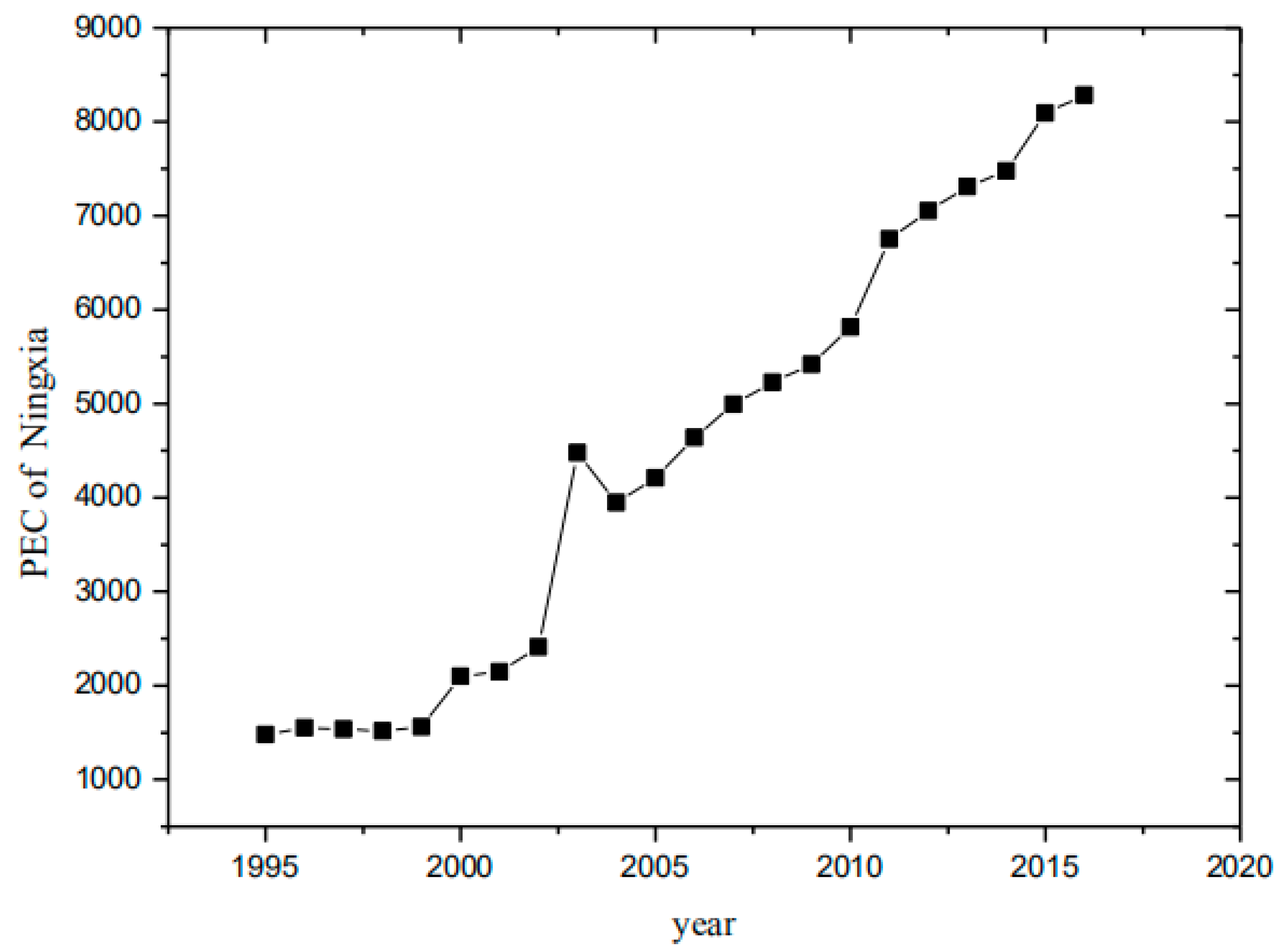
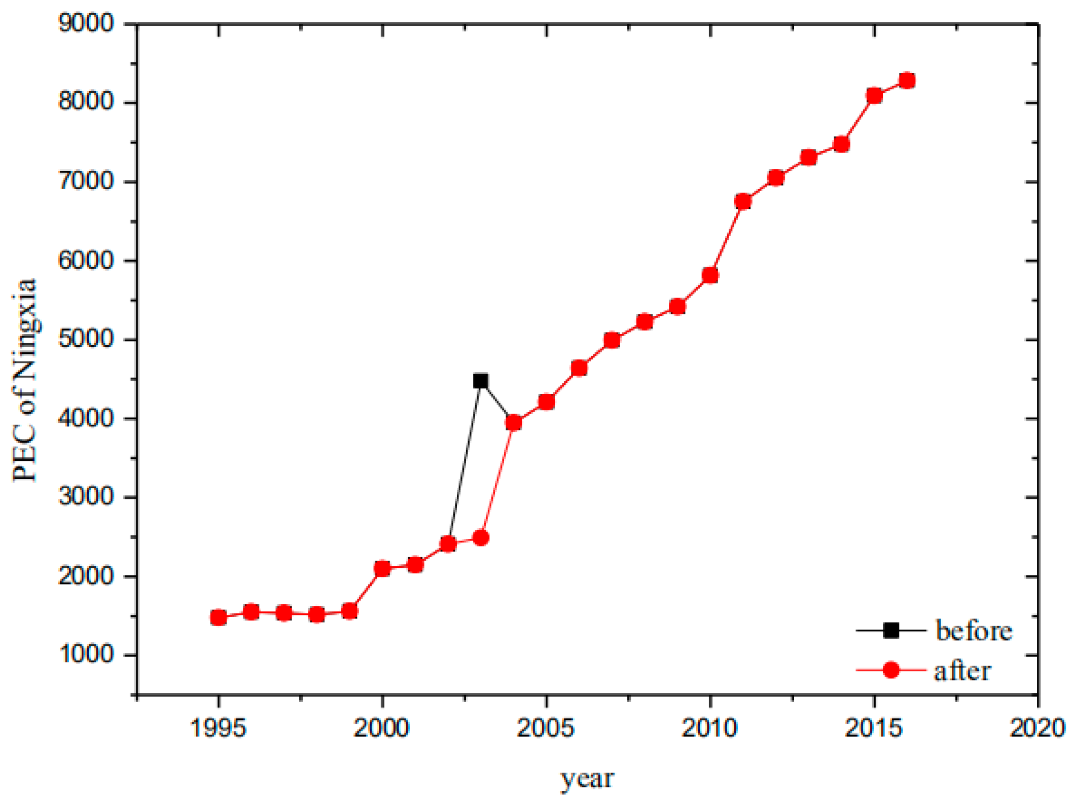
For the time-series data fitting AR (1) model and through the outlier joint estimation diagnostic method, we calculate the τ value of Ningxia Hui Autonomous Region in 2003 and that is 3.97, which is greater than the critical value and identified as a mutational outlier.
(2)
β convergence exists nationwide with a convergence rate of 3.05%. According to the nonlinear time-varying factor model (log-t method), 30 provinces are divided into two convergence clubs. The convergence rate of the first club (high per capita energy consumption) is 4.5%, and that of the second club (low per capita energy consumption) is 6.12%. The convergence rate of the two clubs is higher than that of the whole country.
(3)
Based on the half-life cycle model and the convergence rate, the half-life cycle of the first club is 15 years and that of the second club is 11 years. By constructing the half-life cycle model of β convergence theory, the revised data of the Ningxia Hui Autonomous Region represent 2490.53 kce/person.
(4)
The outliers identified in the paper are likely to be caused by human error, instrument failure and other errors in the process of data collection. This reminds us to attach importance to data collection, strengthen the supervision of data collection, and take measures such as multiple calculations to make the data real and effective.
This study takes China’s per capita energy consumption as the research object, then identifies the outlier and corrects it based on regional convergence theory. Considering the characteristics of geographical distribution in the theory of regional convergence, the similarity within the club is used to correct the process, so as to provide a reference method for improving the stability of data. At the same time, the identification and correction process established in this paper is a set of general theories and has good applicability to other data. However, the correction model proposed in this paper is just a reference method for outliers based on regional convergence theory, indicating that it is not an absolute process. Meanwhile, the stability of specific correction results needs to be further studied.

Author Contributions

Conceptualization, N.L.; methodology, N.L., Y.L. and X.Z.; software, Y.L.; validation, Z.P.; formal analysis, Y.J.; data curation, N.L. and X.Z.; writing—original draft preparation, Y.L.; writing—review and editing, X.J., X.Z. and J.P.; supervision, H.M. All authors have read and agreed to the published version of the manuscript.

Funding

This research received no external funding.

Acknowledgments

We gratefully acknowledge the financial support from the National Natural Science Foundation of China (No. 71603039, 5197602, 71828401). We are grateful to the editors and anonymous reviewers and to all those who have contributed to the improvement of this article.

Conflicts of Interest

The authors declare no conflict of interest. The funders had no role in the design of the study; in the collection, analyses, or interpretation of data; in the writing of the manuscript, or in the decision to publish the results.

References

  1. Solow, R.M. A Contribution to the Theory of Economic Growth. Q. J. Econ. 1956, 70, 65–94. [Google Scholar] [CrossRef]
  2. Baumol, W.J. Productivity Growth, Convergence, and Welfare: What the Long-Run Data Show. Am. Econ. Rev. 1986, 76, 1072–1085. [Google Scholar]
  3. Barro, R.J.; Salaimartin, X. Convergence across States and Regions. Brook. Papers Econ. Act. 1991, 1991, 107–182. [Google Scholar] [CrossRef] [Green Version]
  4. Roe, T. Determinants of Economic Growth: A Cross-Country Empirical Study. Am. Political Sci. Rev. 2003, 92, 145–477. [Google Scholar] [CrossRef]
  5. Chambers, D.; Dhongde, S. Convergence in income distributions: Evidence from a panel of countries. Econ. Model. 2016, 59, 262–270. [Google Scholar] [CrossRef]
  6. Iacovone, L.; Bayardo, L.F.S.; Sharma, S. Regional Productivity Convergence in Peru; Social Science Electronic Publishing: Washington, DC, USA, 2018. [Google Scholar]
  7. List, J.A. Have air pollutant emissions converged among U.S. regions? Evidence from unit root tests. South. Econ. J. 1999, 66, 144–155. [Google Scholar] [CrossRef]
  8. Mishra, V.; Smyth, R. Convergence in energy consumption per capita among ASEAN countries. Energy Policy 2014, 73, 180–185. [Google Scholar] [CrossRef]
  9. Sheng, Y.; Shi, X.; Zhang, D. Economic growth, regional disparities and energy demand in China. Energy Policy 2014, 71, 31–39. [Google Scholar] [CrossRef]
  10. Apergis, N.; Fontini, F.; Inchauspe, J. Integration of regional electricity markets in Australia: A price convergence assessment. Energy Econ. 2016, 62, 411–418. [Google Scholar] [CrossRef]
  11. Solarin, S.A.; Gil-Alana, L.A.; Al-Mulali, U. Stochastic convergence of renewable energy consumption in OECD countries: A fractional integration approach. Environ. Sci. Pollut. Res. 2018, 25, 17289–17299. [Google Scholar] [CrossRef]
  12. Galor, O. Convergence? Inferences from Theoretical Models. Econ. J. 1996, 106, 1056–1069. [Google Scholar] [CrossRef]
  13. Sul, D. Transition Modeling and Econometric Convergence Tests. Econometrica 2007, 75, 1771–1855. [Google Scholar]
  14. Phillips, P.; Sui, D. Economic Transition and Growth. J. Appl. Econom. 2010, 24, 1153–1185. [Google Scholar] [CrossRef] [Green Version]
  15. Kim, Y.S. Electricity Consumption and Economic Development: Are Countries Converging to a Common Trend? Energy Econ. 2015, 49, 192–202. [Google Scholar] [CrossRef]
  16. Parker, S.; Liddle, B. Economy-wide and manufacturing energy productivity transition paths and club convergence for OECD and non-OECD countries. Energy Econ. 2016, 62, 338–346. [Google Scholar] [CrossRef]
  17. Mérida, A.L.; Carmona, M.; Congregado, E.; Golpe, A.A. Exploring the regional distribution of tourism and the extent to which there is convergence. Tour. Manag. 2016, 57, 225–233. [Google Scholar] [CrossRef]
  18. Cuñado, J.; de Gracia, F.P. Real convergence in Africa in the second-half of the 20th century. J. Econ. Bus. 2006, 58, 153–167. [Google Scholar] [CrossRef]
  19. Cuñado, J.; Gil-Alana, L.A.; de Gracia, F.P. Additional Empirical Evidence on Real Convergence: A Fractionally Integrated Approach. J. Econ. Bus. 2006, 142, 67–91. [Google Scholar]
  20. Cuñado, J.; De Gracia, F.P. Real convergence in some Central and Eastern European countries. Appl. Econ. 2006, 38, 2433–2441. [Google Scholar] [CrossRef]
  21. Romer, D. Advanced Macroeconomics, 4th ed.; McGraw-Hill Education: New York, NY, USA, 2001. [Google Scholar]
  22. Seongman, M. Inter-Region Relative Price Convergence in Korea. East Asian Econ. Rev. 2017, 21, 123–146. [Google Scholar] [CrossRef]
  23. Bergman, U.M.; Hansen, N.L.; Heeboll, C. Intranational Price Convergence and Price Stickiness: Evidence from Denmark. Scand. J. Econ. 2018, 120, 1229–1259. [Google Scholar] [CrossRef]
  24. Fox, A.J. Outliers in Time Series. J. R. Stat. Soc. 1972, 34, 350–363. [Google Scholar] [CrossRef]
  25. Tsay, R. Time Series Model Specification in the Presence of Outliers. Publ. Am. Stat. Assoc. 1986, 81, 132–141. [Google Scholar] [CrossRef]
  26. Bruce, A.G.; Martin, R.D. Leave-k-out diagnostics for time series. J. R. Stat. Soc. 1989, 51, 363–424. [Google Scholar] [CrossRef]
  27. Chen, C.; Liu, L.M. Joint Estimation of Model Parameters and Outlier Effects in Time Series. J. Am. Stat. Assoc. 1993, 88, 284–297. [Google Scholar]
  28. Ping, C.; Jing, Y.; Li, L. Synthetic detection of change point and outliers in bilinear time series models. Int. J. Syst. Sci. 2015, 46, 284–293. [Google Scholar]
  29. Yan, H.; Yang, B.; Yang, H. Outlier detection in time series data based on heteroscedastic Gaussian processes. J. Comput. Appl. 2018, 76. [Google Scholar] [CrossRef]
  30. Sathe, S.; Aggarwal, C.C. Subspace histograms for outlier detection in linear time. Knowl. Inf. Syst. 2018, 56. [Google Scholar] [CrossRef]
Figure 1. The per capita energy consumption data of Ningxia (kce/person).
Energies 13 04909 g001
Figure 2. Results of the club grouping.
Energies 13 04909 g002
Figure 3. The per capita energy consumption data before and after correction of Ningxia (kce/person).
Energies 13 04909 g003
Table 1. The per capita energy consumption data of the Ningxia Hui Autonomous Region (kce/person).
YearDataYearDataYearData
19951479.6520034479.3120116750.07
19961552.4020043948.9820127049.54
19971535.8520054211.4120137308.27
19981518.4020064639.0720147476.64
19991561.6920074995.0820158092.77
20002098.6320085225.3420168284.44
20012145.8320095420.25
20022409.0920105815.69
Table 2. The parameters of the autoregressive moving average (ARMA) model.
Case 1Case 2
Model: 1 1 0
Coefficients:
AR: 0.974419 ***
AIC: −0.239257
Model: 0 1 1
Coefficients:
MA: 0.961220 *
AIC: 1.046726
Note: *** and * denote rejection of the null hypothesis at the 1% and 10% levels, respectively.
Table 3. Division and order of clubs in 30 provinces.
Serial NumberProvinceFirst ClubSecond Club
Step 1Step 2Step 1Step 2
1Ningxiabenchmarkcore
2Inner Mongolia−0.1094core
3Qinghai−1.38054core
4Xinjiang−1.1309core
5Tianjin0.617951core
6Shanxi−0.17756core
7Shanghai2.484757core
8Liaoning1.5625811.562581
9Hebei1.2701862.484757
10Shandong1.8482062.055578
11Jiangsu1.7863471.223246
12Zhejiang0.96617−1.00499benchmark
13Heilongjiang−0.57553−6.504691.407396
14Beijing−0.17778−1.130356.157279
15Fujian0.6195551.902167
16Shaanxi1.031260.447247
17Chongqing1.3945790.180409
18Jilin0.763656−3.696675.497718
19Guizhou0.338821−3.595487.292697
20Hubei−0.00855−2.506957.092816
21Guangdong−0.72039−5.460637.795714
22Gansu−1.46008−6.521797.023633
23Sichuan−1.38843−2.090567.041624
24Henan−1.30784−1.773797.538447
25Hunan−0.79085−0.537477.20602
26Yunnan−1.3583−5.717236.881611
27Hainan−1.56274−4.269876.73345
28Guangxi−1.09245−1.04366.628484
29Anhui−1.95887−8.911765.915468
30Jiangxi −4.791335.766989
Table 4. Grouping of clubs.
NumberMembersThe Number of MembersCategory
Club 1Ningxia, Inner Mongolia, Qinghai, Xinjiang, Tianjin, Shanxi, Shanghai, Liaoning, Hebei, Shandong, Jiangsu, Fujian, Shaanxi, Chongqing14High energy consumption
Club 2Zhejiang, Heilongjiang, Beijing, Jilin, Guizhou, Hubei, Guangdong, Gansu, Sichuan, Henan, Hunan, Yunnan, Hainan, Guangxi, Anhui, Jiangxi16Low energy consumption
Table 5. Results of regional convergence test in clubs.
Test ParametersNationwideFirst ClubSecond Club
α0.22110.28340.3011
t-Statistic5.66264.453313.3257
Prob.0.00000.00080.0000
β0.03050.04500.0612
t-Statistic3.08972.19545.7992
Prob.0.00450.04850.0000
R20.38490.50100.8957
Log likelihood83.507440.182559.9100
F-statistic17.521712.0503120.2604
Prob (F-statistic)0.00030.00460.0000
Durbin-Watson stat1.21470.30321.0712
Table 6. Results of the convergence rate and the semi-life cycle in clubs.
ClubClub 1Club 2
β4.50%6.12%
γ9.36288.3233
Half-life cycle (year)1511

