Shaping High Efficiency, High Temperature Cavity Tubular Solar Central Receivers

Abstract

High temperature solar receivers are developed in the context of the Gen3 solar thermal power plants, in order to power high efficiency heat-to-electricity cycles. Since particle technology collects and stores high temperature solar heat, CNRS (French National Center for Scientific Research) develops an original technology using fluidized particles as HTF (heat transfer fluid). The targeted particle temperature is around 750 °C, and the walls of the receiver tubes, reach high working temperatures, which impose the design of a cavity receiver to limit the radiative losses. Therefore, the objective of this work is to explore the cavity shape effect on the absorber performances. Geometrical parameters are defined to parametrize the design. The size and shape of the cavity, the aperture-to-absorber distance and its tilt angle. A thermal model of a 50 MW hemi-cylindrical tubular receiver, closed by refractory panels, is developed, which accounts for radiation and convection losses. Parameter ranges that reach a thermal efficiency of at least 85% are explored. This sensitivity analysis allows the definition of cavity shape and dimensions to reach the targeted efficiency. For an aperture-to-absorber distance of 9 m, the 85% efficiency is obtained for aperture areas equal or less than 20 m² and 25 m² for high, and low convection losses, respectively.

1. Introduction

1.1. Context

Among the various concentrating solar technologies, central receiver (CR) point focusing systems (or solar power tower, SPT) offer a wide range of options, in term of power, working temperature, storage capacity and, as a consequence, conversion efficiency. Typical CR solar power plants, include a heliostat field that focuses the solar radiation onto the aperture of a receiver, located on top of a tower. The receiver absorbs the solar energy and transfers it either to the thermal energy storage or to the power block that converts heat to electricity. State-of-the-art technology uses molten salt as heat transfer fluid, a binary mixture of sodium and potassium nitrates that can operate up to 565 °C. The salt decomposes at higher temperature than 600 °C and freezes at approximately 220 °C. In central receiver systems, the solar receiver is a key component that endures high thermal stresses during heating and cooling phases and that accommodates solar flux density up to 850 kW/m² [1]. Tubular receivers are operated in all the commercial solar thermal power plants even if other options as porous receivers have been developed at pilot scale [1]. Molten salt working temperature results in heat-to-electricity efficiency of approximately 42%. Getting higher efficiencies (~50% and more) is possible at 700–750 °C with supercritical carbon dioxide (sCO₂) cycles [2] and at approximately 850 °C with combined cycles [3]. Such high operating temperatures result in great challenges on the solar receiver design, construction materials and heat transfer fluids. Central receiver designs are, either external or cavity types. At high temperatures, external receiver must tolerate high incident solar flux densities (high concentration, ~1000 suns), in order to maintain acceptable radiation losses [4]. Consequently, high wall-to-fluid heat transfer coefficients are compulsory in external tubular solar receivers to maintain the wall temperature within its allowable working condition as it is the case with liquid sodium [5]. The other option is using direct HTF heating design as falling particles solar receivers [1].

Cavity receiver concepts reduces radiative heat losses, as the mean concentration at the cavity aperture can be much higher than the mean concentration at the solar absorber surface. The design of the cavity receivers requires a compromise between maximizing solar radiation absorption (minimizing spillage) and minimizing radiation and convection losses. The trade-off between aperture size, radiation capture and operating temperature was examined in [6] for a cavity receiver located at the focus of a medium size solar furnace (18.9 kW_th). Researches on cavity receivers have been mainly focused on small-size cavities integrated with dish solar concentrators [7,8,9]. Numerical three-dimensional (3D) study of the combined natural convection and radiation heat losses of downward facing cavity receivers of different shapes was presented in [7], in the temperature range 250–650 °C. The results indicated that convection losses decrease strongly with the inclination angle of the cavity for all the receiver shapes. A correlation was proposed to predict the convective losses in a small range of Rayleigh number (Ra = 2 × 10⁸–6 × 10⁸). Le Roux et al. [8] have studied tubular receiver in the power range of 1–100 kW to be used in a small-scale solar thermal Brayton cycle using a micro-turbine. The numerical study integrated the optical efficiency of a dish concentrator (tracking error) and the thermal efficiency of the receiver. A 3D numerical simulation of cylindrical cavity receivers, with a 45° (π/4 radians), inclination was proposed in [9]. It was shown that the receiver efficiency varied sharply with the aperture size and that the ratio of radiation to convection losses was ranging from approximately two to four at low direct normal irradiance (DNI) (i.e., low temperature), and high DNI, respectively. Grange et al. [10] modeled a medium-scale cavity receiver to power a Brayton cycle. Receiver efficiency of solar power tower was studied for example in [11,12,13,14]. Rodriguez-Sanchez et al. [11] reported an operation efficiency of molten salt external receiver of the Solar Two demonstration power plant. The results showed that receiver efficiency was around 76% for full load and 69% for half load. These data are lower than previous estimations, 87%, and 80% respectively, reported when the external tube temperature was assumed independent of the incident power. Kim et al. [12] developed a simplified model of heat losses of SPT receivers using correlations derived from numerical simulations. External and cavity with a 9 m²-absorber have been considered in the temperature range 600–900 °C. For low wind velocity, calculated efficiency of Solar Two external receiver was 88% [12]. Generally, for cavity receivers at 900 °C the ratio of radiation to convection losses ranged between 2 and 7 except with head-on high wind condition (10 m/s) that resulted in a ratio approximately equal to one [12]. A cavity-type molten salt solar receiver model was developed in [13] in combination with a solar field optical model. The receiver model included a thermo-hydraulic approach of molten salt flow in 12 m-long tubes. Qiu et al. [14] have proposed a similar approach, including a strategy for a direct steam generation cavity solar receiver tested at Dahan pilot-plant (China). They demonstrated that the cavity effect could improve the optical efficiency throughout the whole year. The effect of directional variation of optical properties in cavity solar receiver was discussed in [15] using Monte Carlo simulations. They concluded that the higher the diffuse ratio, the higher the efficiency and the lower the influence of incident radiation pattern.

The estimation of convective losses in cavity solar receivers is still a subject for research, since accurate modelling of natural convection at high Rayleigh numbers is very challenging. Clausing [16,17] developed an analytical approach of convective losses in cavity central receivers and compared the data with experimental results. He considered two zones inside the cavity, a natural convection zone facing the aperture and a stagnant zone at the upper part of the cavity. The heat exchange between air and surfaces (active and inactive) was based on the average bulk air temperature T_b (T_b = (T_c + T_a)/2, where T_c and T_a are the cavity and ambient air temperature respectively). Nusselt number versus Rayleigh number correlations have been deduced for different regimes and cavity orientations. The comparison with experimental data resulted in a convective heat transfer coefficient of 7.2 and 9.7 W/m²K for the inactive, and the absorber tube surfaces, respectively. Samanes et al. [18] compared different correlations for convective losses prediction and selected the Clausing’s approach. A numerical analysis of convective losses of inclined cavity was proposed in [19]. They concluded that in no wind condition the Clausing model and the simulation results match very well (for both horizontal and inclined cavities). For inclined cavity with wind, an increase of the convective losses was predicted due to a shrinking of the stagnant zone, which is in contrast to the predictions of the Clausing model.

Table A1. List of references of convective losses studies in cavity receivers.

Reference	Topic of the Paper	Main Parameters	Results	Correlation
R.D. Jilte et al. [7]	Numerical 3D study of the combined natural convection and radiation losses associated to dish concentrators	T° = [250–650] °C. Cavity inclination: 0 to 90°. Cavity shapes: cylindrical, conical, etc and spherical	Convection losses decrease strongly with the inclination angle of the cavity for all the receiver shapes.	$Nu=0.122R{a}^{0.31}{\frac{T_{wall}}{T_{amb}}}^{0.066}\ast {\left(1+\cos \left(\frac{\pi }{2}-\alpha \right)\right)}^{0.38}$ For Rayleigh number between 2 × 108 and 6 × 108. Standard deviation of 16%.
C. Zou et al. [9]	3D numerical simulation of cylindrical cavity receiver	Cavity inclination: 45°	The receiver efficiency varied sharply with the aperture size. The ratio of radiation to convection losses ranges from approximately 2 to 4 at low DNI and high DNI, respectively.	Ø
J. Kim et al. [12]	Model of heat losses of Solar Power Tower receivers	External and cavity receiver with a 9 m2 absorber T° = [600–900] °C. $v_{wind}$ = [1,2,3,4,5,6,7,8,9,10] m/s, head-on and side-on.	For low wind velocity, calculated efficiency of Solar Two external receiver was 88%. For cavity receivers at 900 °C, the ratio of radiation to convection losses ranged generally between 2 and 7, except with head-on high wind condition (10 m/s) that result in a ratio around 1.	$\frac{Q_{conv}}{Q_{conv}+Q_{rad}}=a\ast ln\left(\frac{S_{ape}}{S_{rec}}\ast T_{rec}^4\ast {10}^{-12}\right)+b$ $a=-4.611\times {10}^{-4}{v}_{wind}^2+5.517\times {10}^{-3}{v}_{wind}-0.1071$ $b=-5.917\times {10}^{-4}{v}_{wind}^2+3.158\times {10}^{-2}{v}_{wind}+0.1190$ Standard deviation of 11.4%.
A.M. Clausing [16]	Analytical approach of convective losses in cavity central receivers	$P_{rec}$ = 1 and 39 MW T° = 920 and 1020 °C $H_{ape}$ = 5.6 and 0.93 m	The influence of the wind on the convective losses at normal operating conditions are small. The inclination of the aperture is critical since it strongly influences the height of the convective zone within the cavity.	Ø
A.M. Clausing [17]		$\alpha$ = 45 and 180° with the vertical Gr = [$1.39\times {10}^9$–$1.24\times {10}^{11}$].	The wind and buoyancy driven bulk flow both appear to have secondary influences for the cubic cavity orientations. There is a strong evidence for the existence of the stagnation zone and the proposed low convective energy flux across the boundary of this zone. The comparison with experimental data resulted in a convective heat transfer coefficient of 7.2 and 9.7 W/m2K for the inactive and the absorber surfaces respectively.	$Nu=0.082R{a}^{\frac{1}{3}}\left[-0.9+2.4\frac{T_{wall}}{T_{amb}}-0.5{\frac{T_{wall}}{T_{amb}}}^2\right]z\left(\alpha \right)$ $z\left(\alpha \right)=\{\begin{array}{c}1 si 0\le \alpha \le 135°\\ \frac{2}{3}\left[1+\frac{\sin \left(\alpha \right)}{\sqrt{2}}\right]\sin \alpha >135°\end{array}$ Factor z added to account for all orientation. Without it, previous authors found absolute deviation of 1%.
J. Samanes et al. [18]	Comparison of correlations for convective losses	Ps-10 like cavity receiver (300 tubes in a 7 m radius and 12 m height, and $P_{rec}$ = 56.7 MW) Five models are compared and validated	Clausing’s model provides the heat losses on each surface of the cavity receiver, and its method is considered as the best choice.	Ø
R. Flesch et al. [19]	Numerical analysis of convective losses	Head-on and side-on wind $\alpha$ = [0–90]°	Clausing’s model is a good approach for natural convection. When no wind is present, the losses decrease considerably with increasing the inclination angle of the receiver.	Ø

, presented in Appendix A, lists the previously cited studies and their main findings.

As discussed previously, the development of high efficiency power cycles requires the use of new heat transfer fluid that could be either high temperature molten salts, high pressure gases or particles [20]. Particles offer the unique set of advantages of high temperature operation, no freezing issues and ability to be used as cheap storage material. Until now, there are three main promising concepts of solar particle receivers. The so-called falling particle receiver developed by Sandia National Laboratory (SNL) [21], the centrifugal receiver proposed by the German aerospace center (DLR) [22] and particles-in-tube (or dense suspension of particles) solar receiver developed by the French National Center for Scientific Research (CNRS) [23,24]. A pilot scale demo-unit is currently under construction within the framework of Next-CSP European projects [25]. The main advantages of the latter concept are the use of a tubular receiver similar to the standard receiver of solar power tower and small diameter particles that exhibit high wall-to-fluidized bed heat transfer coefficient [26]. The main drawback is using an indirect heating configuration of the HTF that results in strong constraints on the absorber wall temperature and in the choice of a cavity receiver concept to reduce the radiative losses.

The previous literature review indicates that studies on the effect of cavity geometry and shape on the efficiency of SPT cavity receivers are very scarce and generally limited to small-scale systems. Moreover, the use of particles as heat transfer fluid leads to specific challenges and constraints that must be examined in details. The inadequate efficiency of large-scale solar receivers working in the temperature range 900–1000 °C presents a challenge. Obviously, the increase in overall solar-to-electricity efficiency of solar power plant, integrating an advanced heat-to-electricity conversion cycle, can be obtained only if the solar receiver efficiency is maintained in the same range as in current molten salt receiver, 85–90%. This is the targeted efficiency in this parametric study. Other specific constraints are justified by previous results and general consideration as explained below.

1.2. Background

The fluidized particle-in-tube receiver concept has been in development since 2010 [27]. The most important characteristics of this concept are the particle flow stability and regime along the tube height and the associated wall-to-fluidized bed heat transfer. The latter governs the acceptable incident solar flux on the tube walls. The working principle of the system is as follows: The bottom tip of the tubes are immersed in a fluidized bed generated in a vessel named “the dispenser”. The upward flow of the particle suspension is controlled by tuning the freeboard pressure in the dispenser. The differential pressure between the bottom (dispenser) and the top of the tube is directly correlated to the particle mass flow rate. The typical pressure drop in the tube is 100 mbar/m. The nominal solid mass flux inside the receiver tubes is limited by the choking phenomena that results in the clogging of the tubes at high solid mass flux. The choking limit depends on the gas velocity and particle properties [28]. Our own experimental results indicate that 250 kg/m²s is a safe limit for 50 mm intern diameter (ID) tubes and approximately 50 μm particles. The particles can experience a different regime along the tube height in particular bubbling and slugging [29]. Axisymmetric slugging must be avoided due to the associated reduction of the particle-to-wall heat transfer coefficient. Fortunately, slugging is strongly reduced with increases in temperature. Nevertheless, this issue results in a limited height of the tubes. General particle flow in each tube in a multi-tube solar receiver [30] is not affected by the presence of adjacent tubes. In particular, any difference in particle mass flow rate was observed. Concerning the maximum power of a single receiver, it is clearly related to the maximum acceptable height of the tubes, this issue is discussed in [31].

The design of solar power plant starts with the prediction of the performances at design point, i.e., at nominal conditions. Then, the time scale is introduced by simulating the plant production during a typical day and year. This paper presents the first step, the receiver design at nominal conditions. This step is necessary to start with the next step, the coupling between the solar field and the solar receiver that governs the overall solar-to-heat conversion efficiency of the system (optical efficiency × thermal efficiency). Moreover, the effect of transients on the receiver thermal efficiency and lifetime is another issue that require thermo-mechanical simulation.

Operating particle solar receivers in a solar thermal power plant requires handling and conveying of a large quantity of powder. This issue is discussed in [32].

Finally, some critical challenges in fluidized particle-in-tube solar receiver development have been identified. Slugging regime must be avoided in order to maintain a constant wall-to-fluidized bed heat transfer coefficient along the tube height. This issue can be solved by operating in the turbulent fluidization regime [33]. The control of incident solar flux distribution on the tube wall is mandatory to avoid hot spots; aiming strategy is proposed in [31]. Thermo-mechanical behavior of the tubes submitted to high thermal gradient between the irradiated front side and the back side as reported in [26] is one of the most critical issue at high temperature. This challenge can be addressed by increasing the particle mixing (see above cited “turbulent fluidization regime [33]”) and the heat transfer coefficient.

1.3. Objective

Consequently, the following assumption are made:

• The acceptable length of the absorber tubes limits the maximum power of the solar receiver. Based on a previous study [29] and further unpublished experimental results, the length of the tubes is fixed at 7 m. Accounting for this limited length of the tubes, the nominal power of a single solar receiver is approximately 50 MW [31].
• The wall-to-fluidized bed heat transfer coefficient is chosen in agreement with previous experimental data [26].
• The tubes are vertical. Vertical position of the absorber tubes is mandatory because tilting will result in a strong channeling and particle segregation. Indeed, this would cause a very non-homogeneous bed, with a dense bed (without bubbles) near the solar-irradiated part of the tube and all the bubbles in the opposite region [34]. This will cause a dramatic decrease of wall-to-bed heat transfer.
• The solar radiation acceptable flux density is another constraint related to the working temperature limit of the tube wall. This value is discussed in the next section.

Section 2 of the paper is devoted to the description of the solar cavity receiver, whose shape can vary, and to preliminary calculations (number of tubes and mean incident solar flux). Section 3 addresses the numerical modelling. The results of the model are presented in Section 4 as well as a discussion on the simulation data. Section 5 focuses on the influence of convective losses and temperature on the receiver efficiency and defines the parameters to respect in order to reach the targeted receiver thermal efficiency of at least 85%.

2. Receiver’s Geometry and Preliminary Considerations

2.1. General Description and Material Properties

The absorber is a key component of a solar tower power plant. Its main functions are: (i) to receive the concentrated solar flux, (ii) to be able to withstand the required operating temperature, and (iii) to transfer the produced heat to the heat transfer fluid as efficiently as possible. Its design results from a trade-off between the necessity to properly direct the concentrated solar flux from the heliostats to the absorber, to avoid tubes overheating (and thus open the cavity), and the thermal losses limitation (which tends to limit the cavity aperture dimension). For north-facing solar tower, the absorber takes the form of a semi-circular cavity in which cylindrical tubes are installed side-by-side. The heat transfer fluid (here fluidized bed) circulates in the later to extract the incident solar power.

Due to size constraints, the space between the tubes is very small and is assumed to be zero in the rest of the study. Furthermore, the tubes are assumed to behave as flat receiving walls, placed in a cavity in the shape of an arc of a circle (Figure 1). These walls are said to be “active” because they transmit the received solar radiation to the HTF. In order to avoid fluidization issues, these tubes are always positioned vertically (see Introduction). “Passive” refractory panels close the cavity (in blue in Figure 1). Under the effect of the incident radiation, the temperature of the active walls rises and heat transfer occurs between the tube walls and the fluidized particles (useful power) and within the cavity. The latter is composed of convection losses between the cavity air and the walls and of thermal radiation with the rest of the cavity. Part of the radiation from the passive surfaces is directed to the absorber and to themselves, and the rest escapes through the aperture. The fraction of radiation from the passive surfaces and the solar radiation, reflected by the absorber and which moves through the aperture, constitute the radiation losses.

The following assumptions are made to focus the study on the main design issues: The space between the tubes and the rear face of the cavity is considered null and the insulation of the rear faces is considered perfect. The passive walls are made of low absorption material in the solar spectrum that reflects the radiation towards the cavity. These passive surfaces are also thermally insulated from the ambient. In order to evaluate the convective losses on these surfaces, the conduction through the passive walls and their insulation is taken into account.

Finally, the cavity is necessarily opened so that the concentrated solar flux can irradiate the receiver’s tubes. The sunspot shape and the flux distribution on the absorber is controlled by the heliostat field layout and the heliostat orientation (aiming strategy). Optimizing the incident solar flux is out of the scope of this study. The input solar flux is selected a-priori, but is feasible in practice with a current heliostat field management technique [31].

Common materials used in commercial solar power plant have been selected for our study. The cylindrical tubes are made of Inconel 601 (an alloy of Nickel and Chromium) [35,36], and covered with a layer of Pyromark 2500©, a highly absorbent black paint [37,38]. Reflective surfaces are considered in Scuttherm [39] (others possible insulating materials are for example the Promaform [40] or the Insulfrax [41]). The properties of these materials in the solar and infrared spectral bands are presented in

Table 1. Properties of materials used, from literature data [35,36,37,38,39].

	$\mathbf{Absorptivity}{\mathit{\alpha }}^{\mathit{s}\mathit{o}\mathit{l}}$	$\mathbf{Reflectivity}{\mathit{r}}^{\mathit{s}\mathit{o}\mathit{l}}$	${\mathit{\alpha }}^{\mathit{I}\mathit{R}}$	${\mathit{r}}^{\mathit{I}\mathit{R}}$	$\mathbf{Emissivity}{\mathit{\epsilon }}^{\mathit{I}\mathit{R}}$	$\mathbf{Density}\mathit{\rho }$ (kg/m3)	$\mathbf{Thermal}\mathbf{Conductivity}\mathit{\lambda }$ (W/mK)
Absorbent Surfaces	0.9	0.1	0.85	0.15	0.85	8110	26.1
Reflective Surfaces	0.22	0.78	0.95	0.05	0.95	315	0.1

.

The heat transfer fluid is olivine fluidized by an air stream. The later have been selected for their excellent thermal and fluidization properties (group A of Geldart classification) [42,43]. The particle density is 3300 kg/m³ and its specific heat variation with temperature is given by Equation (1). An apparent specific heat is calculated, based on the average temperature of the particle in the tube ($T_{ave}=$ 650 °C), which gives $C_{p,olivine}=$ 1.3 kJ/kgK:

$$C_{p,olivine}=9.70\times {10}^{-8}{T}_{ave}^3-2.62\times {10}^{-4}{T}_{ave}^2+0.73T_{ave}+8.06\times {10}^2.$$

(1)

The receiver geometry is parametrized to explore the cavity shape effect on the absorber performance.

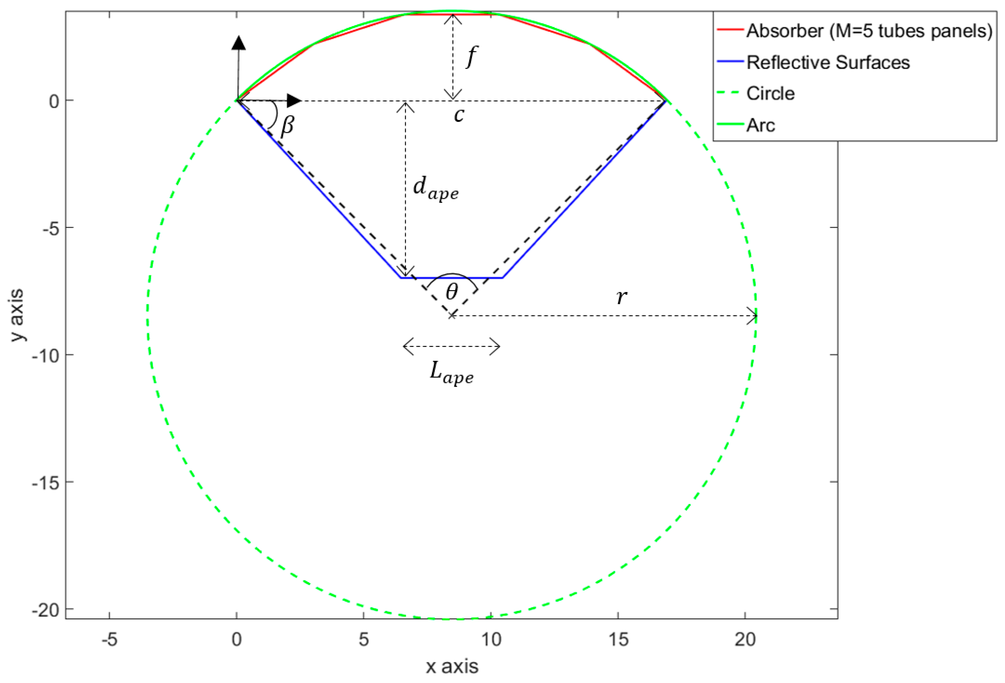
2.2. Geometry Parametrization

2.2.1. The Absorber

The cavity consists of a semi-cylindrical bottom and passive surfaces limiting the aperture. The circular arc is discretized into $M$ segments, each containing $N$ tubes (Figure 2). The geometry of the circular arc is characterized either by a radius of curvature $r$ and an arc angle $\theta$, or by the chord ($c$) and the arrow ($f$) of the two ends (see Figure 2).

Before every calculation, a geometry definition procedure is applied. The left end of the absorber defines the origin of the mark. The positions of the $M+1$ arc base points are calculated from the arc center point $\left(\frac{c}{2},-\left(r-f\right)\right)$ by applying a clockwise rotation of radius $r$ and angle $\theta /M$. As the geometry of the tubes is fixed and their number calculated a-priori to meet the objective of a 50 MW solar receiver, the radius of the arc corresponds to the minimum radius required to encompass all the $N_t$ tubes in the cavity (Equation (2)). Here, $D_t$ is the internal tube diameter of 50 mm and $e_t$ is the tube thickness, 2 mm. The cavity geometry effect is thus explored by varying two parameters {$M$,$\theta$}. The parameters are linked together by the following equation:

$$r=\frac{N_t\left(D_t+2e_t\right)}{M\sqrt{2\left(1-\cos \left(\frac{\theta }{M}\right)\right)}}.$$

(2)

2.2.2. The Aperture

The receiver aperture is square or rectangular, of length $L_{ape}$ and of height $H_{ape}$, and is placed at a distance $d_{ape}$ from the absorber central axes. While, the absorber is inevitably oriented vertically, the aperture may be tilted with respect to the vertical, by an angle $\alpha$, to orient it with respect to the mean axis of the heliostat field. Figure 3 shows this inclination with a schematic sectional view of the cavity, with the associated quantities. In this figure, the vertical plane of the absorber is shown in red, the top and bottom passive surfaces in blue, and the aperture is shown in black, tilted with respect to the horizontal (dotted lines) at an angle $\pi /2-\alpha$. The aperture tilt angle is defined such that it equals to 0 when the aperture is parallel to the absorber.

When the aperture is tilted, new geometrical parameters are derived using Equations (3) and (4), needed to determine aperture vertices:

$$H_{\alpha }=\frac{H_{ape}}{2}\left(1-\cos \alpha \right)$$

(3)

$$d_{\alpha }={\left[H_{\alpha }\left(H_{ape}-H_{\alpha }\right)\right]}^{\frac{1}{2}}.$$

(4)

With these considerations, three angles can be derived to describe the cavity geometry. The angle between the vertical absorber plane and the passive vertical surfaces, $\beta =\mathrm{atan}\left(\frac{2d_{ape}}{c-L_{ape}}\right)$ (see Figure 2), and the angles between the absorber plane and the top, and bottom passive surfaces, respectively ${\gamma }_h=\mathrm{atan}\left(\frac{d_{ape}}{H_t-H_{ape}}\right)$ and ${\gamma }_b=\mathrm{atan}\left(\frac{d_{ape}-d_{\alpha }}{H_{\alpha }}\right)$ (see Figure 3).

The aperture is thus defined by four different parameters: $d_{ape}$, $\alpha$, $L_{ape}$, $H_{ape}$. Prior to any calculation the different geometry vertices and surfaces are numbered and set in a Matlab program.

2.3. Tubes Number Calculation

The tube number in the absorber is calculated based on the extracted power objective. The later can be simply formatted based on a thermal balance on the particles in a tube (Equation (4)), or based on the targeted efficiency,

$${\varphi }_{abs}=\dot{m_p}{N}_t{C}_{p,part}\left(T_{part}^{out}-T_{part}^{in}\right)$$

(5)

where $\dot{m_p}$ denotes the particle mass flow rate per tube, $N_t$ the number of tubes, $C_{p,part}$ the specific heat of the particles (see Section 2.1), and $T_{part}^{in}$ and $T_{part}^{out}$ are, respectively, the inlet and outlet HTF temperature. The latters are fixed in our study to 550 °C and 750 °C respectively to fit with the temperature needed for a sCO₂ cycle [44]. Alternatively, the extracted power can be formulated based on the targeted efficiency ${\eta }_{rec}$ and the incident solar radiation power $P_{rec}$ as follow: ϕabc = η_rec P_rec.

Considering the maximal value for the particle mass flux $G_p=\dot{m_p}/\left(\frac{\pi D_t^2}{4}\right)$ of 250 kg/m²s, with $D_t$ the internal tube diameter (50 mm), an extracted power of 50 MW_th, the targeted efficiency of 85% and equalizing the two formulations, one obtains a total tube number of 360. This value is kept constant in the whole analysis. The chosen particle mass flux, 250 kg/m²s, is a tradeoff between very high values that can result in chocking and small values that will not satisfy the constraint on power extraction and that are difficult to stabilize. Moreover, we have tested this mass flux with a cold mockup. The pressure loss in the absorber does not change with the particles mass flow rate, because the driving force is the pressure inside the dispenser, as explained in the Section 1.2 (Background). The pressure loss depends on the mean particle volume fraction, which is approximately 30%.

2.4. Incident Concentrated Solar Flux

The second parameters to be predefined is the incident concentrated solar flux. The latter has to be high enough to fulfill the extracted power objective but low enough to avoid hot spot leading to the absorber damage. A simple analysis allows setting its value. First, the extracted power is expressed with respect to wall-to-fluidized bed heat transfer coefficient (Equation (6)), estimated to $h_{t,part}=$ 1200 W/m²K based on experimental data [26]. In practice, this coefficient is based on the mean logarithmic temperature difference in the tube and an exchange surface $A_t=\frac{\pi }{2}{D}_t{H}_t$, corresponding to the irradiated part of the exchange surface of the tube. This mean logarithmic temperature difference involves the tube wall temperatures at the inlet and outlet of the particles. For the sake of simplicity, no temperature variation along the tube wall is considered, which simplifies the formulation (Equation (7)):

$${\varphi }_{abs}=h_{t,part}{A}_t\mathsf{\Delta }{T}_{lm,part}$$

(6)

$$\mathsf{\Delta }{T}_{lm,part}=\frac{\left(T_{wall}^{in}-T_{part}^{in}\right)-\left(T_{wall}^{out}-T_{part}^{out}\right)}{\ln \left(\frac{T_{wall}^{in}-T_{part}^{in}}{T_{wall}^{out}-T_{part}^{out}}\right)}\approx \frac{T_{part}^{out}-T_{part}^{in}}{\ln \left(\frac{T_{wall}-T_{part}^{in}}{T_{wall}-T_{part}^{out}}\right)}.$$

(7)

By equalizing this formulation with the extracted power based on the targeted efficiency, ${\varphi }_{abs}={\eta }_{rec}{A}_t{\phi }_{inc}$, one can express the tube wall temperature as a function of the incident solar flux (Equation (8)). Figure 4 displays the wall temperature evolution. Equalizing Equation (5), for a one-tube thermal balance, with the thermal power based on the targeted efficiency and the given solar flux density, leads to an expression of the outlet particle temperature. Inserting the later in Equation (8) gives a new formulation of the wall temperature, which highlights a linear dependency with respect to ${\phi }_{inc}$. Such relationship is in accordance with the plot in Figure 4:

$$T_{wall}=\frac{T_{part}^{out}\ast e^x-T_{part}^{in}}{e^x-1}, withx=\frac{h_{t,part}\left(T_{part}^{out}-T_{part}^{in}\right)}{{\eta }_{rec}{\phi }_{inc}}$$

(8)

The thermomechanical stresses of Inconel 601 impose a wall temperature limit of 1000 °C. This temperature is reached for 480 kW/m². Given the high temperatures involved and the cavity effect, which will increase the net flux received by the absorber, the incident concentrated solar flux density is set to 400 kW/m² in this study. The latter corresponds to a wall temperature of approximately 950 °C.

With such wall temperature level, the radiation emission of the absorber surface, given by ${\epsilon }_{IR}\sigma T_{wall}^4$, equals 108 kW/m² which corresponds to roughly 27% of the incident solar radiation. Such order of magnitude unquestionably legitimates the choice of a cavity type receiver and the need for a geometrical optimization of the cavity to lower the radiation losses.

3. Numerical Modelling

3.1. Radiative Balance

The absorbent surfaces are submitted to concentrated solar power. Most of this radiation is absorbed by the tubes and heats the olivine particles. The tubes reflect part of this incident radiation and emit infrared radiation because of their temperature. The sum of the two fluxes, for a surface i, is the radiosity $J_i$. As the surfaces are considered as gray body in spectral bands, the radiosities in the solar ($300 \mathrm{nm}\le \lambda \le 3000 \mathrm{nm}$) and infrared ($\lambda \ge 3000\mathrm{nm}$) spectral bands may be separated, leading to total radiosities $J_i^{tot}=J_i^{sol}+J_i^{IR}$ (Equations (9) and (10)):

$$J_i^{sol}=r_i^{sol}\left({\phi }_{inc,i}+{\displaystyle \sum }_j{J}_j^{sol}{F}_{ij}\right)$$

(9)

$$J_i^{IR}={\epsilon }_i^{IR}\sigma T_{wall,i}^4+r_i^{IR}{{\displaystyle \sum }}_j{J}_j^{IR}{F}_{ij}.$$

(10)

In these equations, $F_{ij}$ designates the view factor between the surfaces i and j, i.e., the fraction of the flux density emitted by i and received by j. By definition, this term is a double integral, which only depends on the surfaces’ geometry. Functions implemented in Matlab allow calculating the view factors between plane polygons by entering the coordinates of their vertices [45]. Then, to calculate the radiosities of the involved surfaces, Equations (9) and (10) are written to obtain a matrix system of the form $AJ=B=>J=A^{-1}B$ (cf. Appendix B for the details of the $A$ and $B$ terms).

3.2. Losses and Efficiency

3.2.1. Absorbed Power

This model assumes that steady state is reached (i.e., a thermal equilibrium), and the wall temperatures are estimated according to preliminary calculations (see Section 2). Thus, one can express the power absorbed by the particles ${\varphi }_{abs}$ based on their temperature and mass flow (Equation (11)):

$${\varphi }_{abs}=G_p\frac{\pi D_t^2}{4}{N}_t{C}_{p,part}\left(T_{part}^{out}-T_{part}^{in}\right).$$

(11)

3.2.2. Radiative Losses

The radiative losses are calculated from the radiative balance, and represent the radiation which gets out from the cavity through the aperture, here referred to the “0” surface (Equation (12)), where $S_j$ the area of the jth surface:

$${\varphi }_{loss,rad}={{\displaystyle \sum }}_j{S}_j{F}_{j0}{J}_j=S_0{{\displaystyle \sum }}_j{F}_{0j}{J}_j.$$

(12)

3.2.3. Convective Losses

As discussed in Section 2, there are two kind of convective losses in this system.

First, the convective exchanges inside the cavity between active and passive surfaces and air (Equation (13)). The space between the tubes and the rear face of the cavity being very narrow, natural convection is neglected there. The cavity’s convective exchange with the active surfaces are thus the irradiated part of the tube. In the Clausing’s model [16,17], the cavity is split into two zones, separated with a horizontal border which corresponds to the aperture top limit. Above this border, the air is stagnant, its temperature is high and the convection exchange with the walls of the receiver is very low. Then, below the border, the convection is stronger because the air is moving. The fresh air is entering the cavity by the lower part of the aperture, is heated by convection and comes out by the upper part of the aperture. Negligible mixing occurs with the stagnant zone due to the change of the air density with temperature. According to [19], the Clausing’s model allows evaluating the natural convection in the cavity. However, in the case of forced convection, i.e., when there is some wind, the cavity is split into three zones, stagnant and strong convection zones, as in the Clausing’s model, but also with an intermediary transition zone, whose thickness depends on the aperture inclination and the wind velocity. Then, the aperture inclination affects the position of the border between the two (or three) convection zones, and increasing the tilt will increase the convection losses. In the no-wind case, i.e., with natural convection only, the Clausing’s model estimates the air temperature inside the cavity by the mean temperature between the walls and the air outside the cavity, $T_{ext}$. With an outside temperature of 15 °C and walls temperature of 950 °C, as estimated in Section 2, it leads to $T_{air}^{cav}=\frac{T_{wall}+T_{ext}}{2}\approx$ 500 °C.

Second, the convective exchanges with the ambient air, at the back-face of the passive surfaces. The thermal conduction through these elements leads to outside wall temperature $T_{wall}^{ext}$ higher than the ambient air temperature, which results in convective heat transfer (Equation (14)). To simplify the estimation, we arbitrarily consider outside walls temperatures of 150 °C. For an insulation thickness of 0.1 m, the conductive flux through the passive elements does not exceed 10⁻⁵ of the receiver power. Such order of magnitude justifies neglecting this term in the model:

$${\varphi }_{loss,conv}^{cav}={\displaystyle \sum }_i{S}_i{h}_{air}^{cav}\left(T_{wall,i}-T_{air}^{cav}\right)$$

(13)

$${\varphi }_{loss,conv}^{ext}={\displaystyle \sum }_j{S}_j{h}_{air}^{ext}\left(T_{wall,j}^{ext}-T_{ext}\right).$$

(14)

In Equations (13) and (14), $S_i$ is the overall surface area of both active and passive surfaces. We neglected the difference between inside and outside areas.

The convective exchange coefficients h_air in Equations (13) and (14) is not the same for active and passive surfaces according to Clausing (see Introduction). However, as explained in the Introduction, the estimation of convective losses in cavity solar receivers is a challenging subject and thus, the two convective exchange coefficients are assumed to be identical to focus on the scope of this study, which is to assess the influence of the receiver geometry on its efficiency. It is set to 10 W/m²K for the whole study; this value overestimates the convective losses. The effect of this assumption on the simulation results is discussed in Section 5.

3.2.4. Receiver Power and Efficiency

The power entering the solar receiver, $P_{rec}$, is equal to the sum of the exchanged powers (Equation (15)). The efficiency of the receiver ${\eta }_{rec}$ is the ratio between the power absorbed by the particles and $P_{rec}$ (Equation (16)). In the same way, the radiative and convective losses are the ratios between their corresponding power and the receiver power, and the sum of the losses and the efficiency is equal to 1. Here, the flux density distribution is not taken into consideration. We consider a mean solar flux density, as explained in Section 2.4:

$$P_{rec}={\varphi }_{abs}+{\varphi }_{loss,rad}+{\varphi }_{loss,conv}$$

(15)

$${\eta }_{rec}=\frac{{\varphi }_{abs}}{P_{rec}}.$$

(16)

4. Results

The following assumptions are included in the simulations:

• The incident flux on the absorber tubes is 400 kW/m² and the active and passive surfaces wall temperatures are homogenous and equal to 950 °C (see preliminary calculations).
• The ambient air temperature is set at 15 °C while the air temperature inside the cavity is set to 500 °C.
• The total number of tubes N_t is set at 360 but is rounded to have a ratio N_t/M as an integer.

The three parameters, estimated in the previous sections, are considered as constraints in our study.

4.1. Influence of the Absorber Geometry

The angle $\theta$ of the circular arc in which the absorber is inscribed (see Figure 2) was varied for several values of the panels’ number ($M$). The angle ranged from π/6 to π in radians. For each value, the radius of curvature of the arc and the parameters {$c$,$f$} are calculated (see Equation (2)). For the example shown in Figure 5a–c, the following parameters are fixed: The aperture to receiver distance d_ape = 7 m, the aperture length L_ape = 4 m and height H_ape = 5 m, for a zero inclination (i.e., an aperture parallel to the absorber).

The evolution of the radiative and convective losses, as well as the receiver efficiency, as a function of the arc angle (with M as a parameter), are shown in Figure 5. In Figure 5c, which represents the evolution of the receiver efficiency, three shapes of the receiver are inserted as sub-figures. They correspond to $\theta$ values of π/6, π/2 and π respectively for $M=$ 5. The absorber is represented in red along the arc (in green), and the vertical passive surfaces are in blue. The smaller the angle, the larger the radius of curvature is to house the $N_t$ tubes inside the receiver. It varies between 5 and 36 m, which corresponds to a variation of the distance between the two extremities of the absorber (the chord, $c$) between 12, and 18.5 m, respectively. Consequently, the angle $\beta$ between the vertical plane of the absorber and the passive surfaces varies between 44 and 60° (i.e., between 0.77 and 1.05 rad). The angle ${\gamma }_h$ between absorber and the upper passive surface is 74° (1.29 rad), and the angle ${\gamma }_b$ with the lower passive surface is zero since the aperture is not inclined. The power of the receiver varies very slightly for each case, and remains close to the expected 50 MW_th.

Figure 5 indicates that both types of losses are influenced by the receiver geometry, but the change in the receiver efficiency is limited to less than 1% in the range of variation of the parameters. The radiative losses tend to decrease with the increase of the arc angle, while the convective losses reach a maximum around 2π/3 (≈2 rad). Indeed, the increase of the arc angle results in an increase of the top and bottom passive panels that are at the same side as the absorber (with positive values of the y axis on the Figure 5c’s sub-figures), while it decreases the other top and bottom, and the left and right passive areas. Since the decrease of related areas is larger than the increase one, the convective losses decrease, until the threshold value of θ ≈ 2 radians. After this limit, the two losses decrease, which results in an increase of the receiver efficiency. The convective losses reach approximately 5% of the receiver power, which is approximately half of the radiative losses. According to these results, it might be reasonable to work with a fixed arc angle of π, but since the cross section of the absorber is a semicircle, it will be difficult to irradiate the sides located on the edges with the heliostats field. Consequently, the value π/2 seems more realistic considering that a coupling with the heliostat field (optical model) should be added to take into account this phenomenon. In the following calculations, the values π and π/2 are considered.

We do not observe a clear tendency with respect to the number of panels. Values up to $M=$ 21 have been tested, but results are not shown here for the sake of clarity. The simulation data differs by less than 1%. Increasing the number of panels results in a finer precision, since the absorber geometry tends to fit more and more the arc of circle. Nevertheless, in practice, it is complicated to arrange tubes on too many panels. Furthermore, those tubes are immersed in a “dispenser” fluidized bed. Connection constraints between the tubes and the dispenser fluidized bed limits the $M$ number. In the following calculations, the realistic value of $M=$ 5 is set. As a conclusion, our calculations indicate that, for the assumed aperture’s dimensions, the arc geometry of the absorber has a very small effect on the performances of the receiver.

4.2. Influence of the Aperture’s Distance

The distance between the aperture and the absorber, $d_{ape}$ was varied between 1 and 10 m. We consider the same parameters as above, an aperture area of 20 m², an arc angle $\theta =$ π or π/2 and a number of panels $M=$ 5. Correspondingly, the angle $\beta$ between the absorber and the vertical passive surfaces varies between 9 and 68° (i.e., between 0.16 and 1.19 rad), and the angle ${\gamma }_h$ with the top passive surface varies between 27 and 79° (i.e., between 0.47 and 1.38 rad). Figure 6 depicts the changes in the losses and efficiency.

To highlight the shape variations induced by $d_{ape}$, two “extreme” receiver shapes are presented as sub-figures of the Figure 6c. They correspond, respectively, to an aperture-absorber distance of 2, and 9 m, for $\theta$ value of π/2 and $M=$ 5 tubes panels. Figure 6 shows that the distance between the aperture and the absorber has a strong effect on the receiver efficiency because it drastically affects the radiative losses. Increasing $d_{ape}$ results in a decrease of the view factor between the absorber and the aperture, causing a decrease in the radiative losses. Conversely, the same variation of $d_{ape}$ corresponds to an increase of the surface area of the passive surfaces to an increase in the convection losses. The former remains greater than the latter for any $d_{ape}$, thus the receiver efficiency increases with $d_{ape}$. However, as discussed in the previous paragraph, the constraint linked to the integration of the solar field and the receiver leads to a compromise on the value of $d_{ape}$. $d_{ape}=$ 7 m seems to be a reasonable compromise.

Regarding the circular arc angle reduction, a slight decrease in the efficiency is observed, however the latter does not exceed 1%. Nevertheless, the two values are used in the following calculations for the comparison between the optimum value from a purely thermal point of view (π), and a more practical value (π/2).

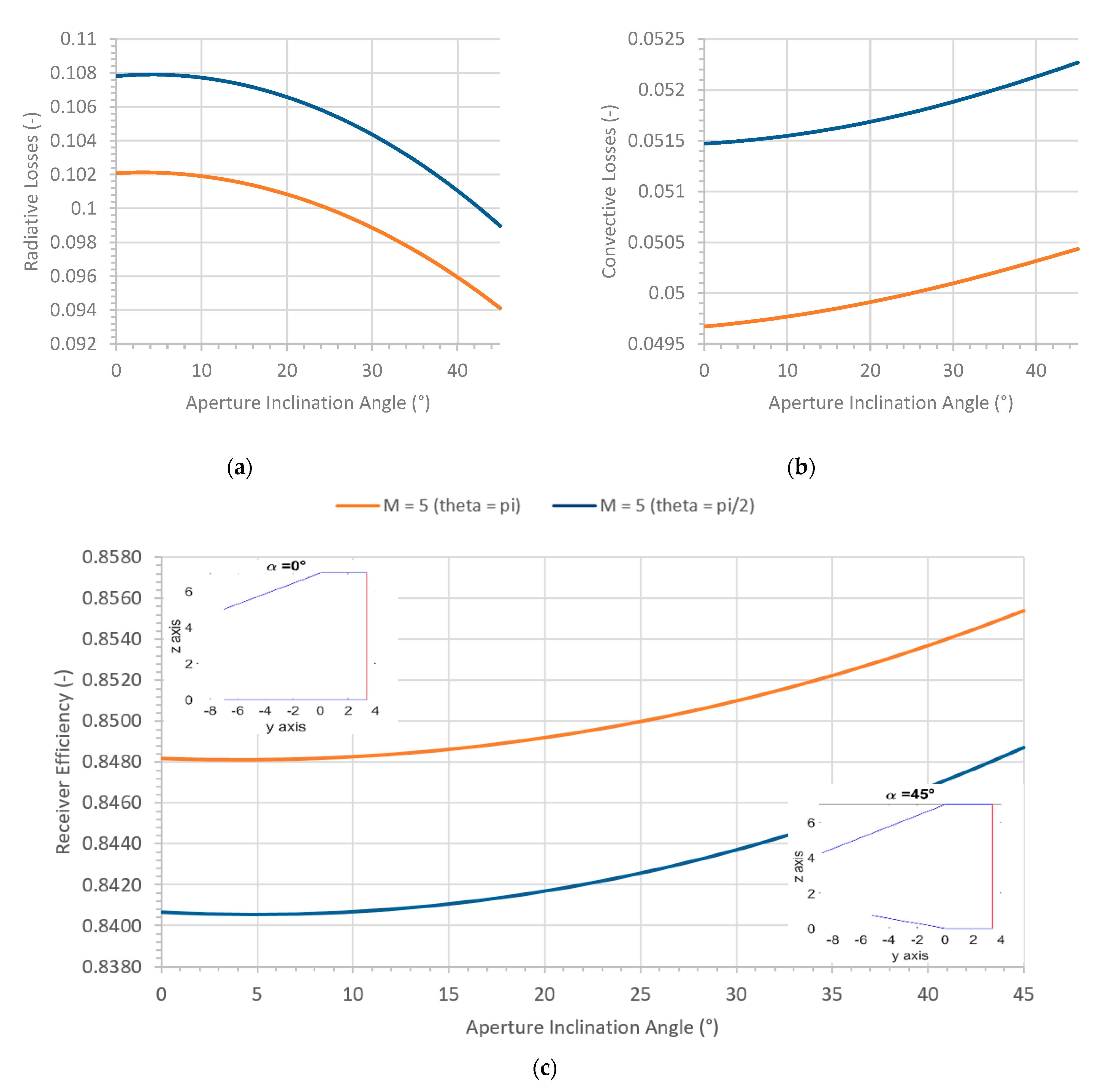
4.3. Influence of the Aperture Inclination

The effect of the inclination angle of the aperture relative to the vertical plane of the absorber, $\alpha$, is discussed in this section. The values of the other parameters are fixed, arc angle $\theta =$ π or π/2, number of panels $M=$ 5, and distance $d_{ape}=$ 7 m. The changes in the different losses and efficiency are presented in Figure 7, with an angle α that varies between 0 and 45° (π/4 radians). This corresponds to variations of the angle ${\gamma }_b$ between the absorber and the bottom passive surface in the range 82–90° (i.e., the range 1.43–1.57 rad), an angle ${\gamma }_h$ of 74° (1.29 rad) and an angle $\beta$, with the vertical passive surfaces, of 47 or 60° (i.e., 0.82 or 1.05 rad), depending on the case π/2 or π, respectively.

In Figure 7c, which represents the evolution of the receiver efficiency, two side views of the receivers are represented as sub-figures, corresponding, respectively, to $\alpha$ = 0 and 45°, in the case of $M=$ 5 and $\theta =$ π/2. In these sub-figures, the absorber panel is in red, and the passive surfaces in blue.

Significant decrease of the radiative losses is observed with the increase of the tilt angle $\alpha$. Despite the increase in the convective losses, the latter remains much smaller than the radiative losses, and the efficiency of the receiver increases with α. Indeed, increasing the inclination of the aperture (while keeping its surface area of 20 m² unchanged) strongly decreases the view factor between the absorber and the aperture, which strongly decreases the radiative losses, while it slightly increases the dimensions of the passive surfaces, which corresponds to the small increase in convective losses.

The coupling of the solar receiver with the solar field must be considered. Even if, from the thermal point of view, a maximal tilt angle is optimal, it might not allow direct solar radiation to reach the entire absorber surface, due to the dependence in its distribution on the height of the receiver and the distance to the central point of the heliostats field. Based on those considerations, the tilt angle selected for the rest of the study is an $\alpha$ of 30° (or π/6 radians), which corresponds to a suitable value for solar power tower.

Regarding the effect of the arc angle $\theta$, there is a slight increase of the receiver efficiency with $\theta$.

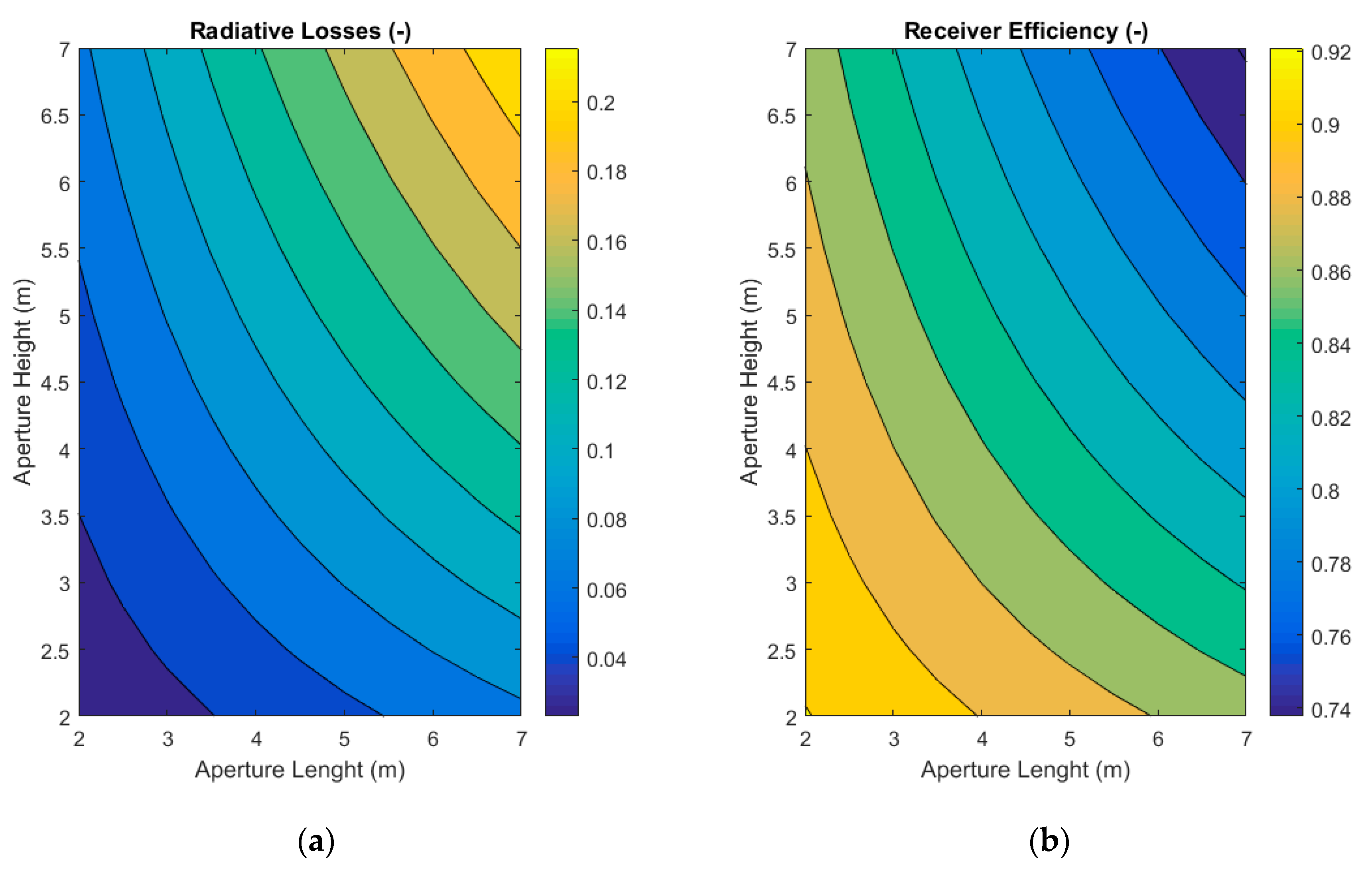
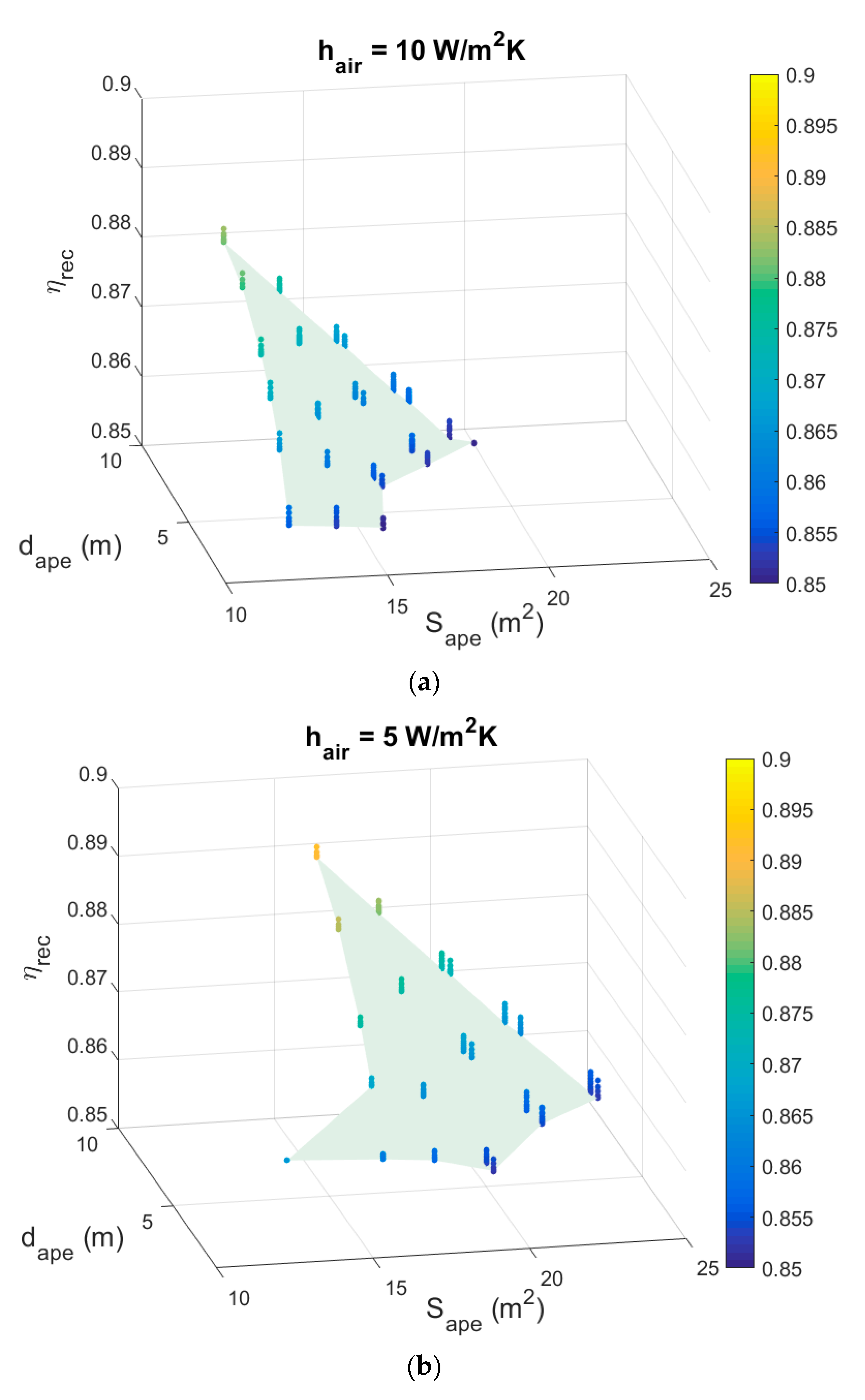
4.4. Influence of the Aperture Dimensions

In this section, the dimensions of the aperture, height $H_{ape}$ and length $L_{ape}$, are assessed while maintaining a rectangular shape. The previous selected parameters are maintained, an arc angle $\theta =$ π/2, a number of panels 5, a distance d_ape = 7 m and an aperture inclination angle $\alpha =$ 30°. Figure 8 shows the evolution of the different losses and efficiency. The angles $\beta$,${\gamma }_h$ and ${\gamma }_b$ range from 43 to 54° (i.e., from 0.75 to 0.94 rad), from 54 to 90° (i.e., from 0.94 to 1.57 rad), and from 85 to 89° (i.e., from 1.48 to 1.55 rad) respectively.

Obviously, the efficiency is maximum for the smallest aperture. However, flux distribution constraints on the absorber must be kept in mind to attain a realistic size. The convective losses are not presented in the figure because they remain almost constant, roughly 5% for all the aperture sizes, while the radiative losses range from 2.31% to 21.54% in the studied domain. Increasing the dimensions of the aperture results in a slight decrease of the passive surfaces areas, and therefore the convection within the cavity also slightly increases. Figure 9a illustrates the evolution of the efficiency and losses as a function of the area of the aperture, $S_{ape}$. The minimum limit of 85% is reached for an aperture area of approximately 20 m².

The mean concentration ratio at the aperture in the studied range of aperture area varies from approximately 1000 to more than 10,000. The latter value is not attainable in commercial scale solar tower. For 20 m² and 25 m² aperture areas, the corresponding concentration ratios are approximately 2500 and 2000 respectively. These values are realistic but are attainable only with high quality (optical and mechanical) heliostats.

Figure 9b plots the receiver efficiency for three shapes, square, vertical rectangle and horizontal rectangle with the aperture surface area as parameter. The three shapes are defined by the ratio between the height and the length of the aperture. It indicates that the shape of the aperture has only a slight influence on the receiver efficiency for a given aperture area. Indeed, the modification of the aperture shape slightly changes the areas of the passive surfaces, which affects the losses. Even if the losses are not strongly influenced by the aperture shape, it has an impact on the solar flux distribution on the absorber from the heliostats field. Due to the absorber dimensions (i.e., the distance between its two extremities of 16.9 m with the parameters fixed previously and a height of 7 m), it makes more sense to choose a horizontal aperture tilt to properly directly radiate the entire absorber surface.

5. Discussion

As discussed in Section 3.2.3, there is large uncertainty on the calculation of convective losses. All the previous simulations have been performed with a convective heat transfer coefficient of 10 W/m²K applied on all the internal surface area of the receiver, including active and passive surfaces at 950 °C. This coefficient value is the maximum given by Clausing [16,17]. Other considerations lead to the conclusion that convective losses have probably been overestimated. First, the inclination of the aperture (Figure 7a–c) results in the formation of a stagnant zone in the upper part of the receiver. Consequently, convective losses are very small in this region. Second, the literature review presented in Section 1.2 (Background) indicates that at high temperature the ratio of radiation to convection losses is approximately 4, whereas in our simulation it is approximately 2. Consequently, additional calculation have been performed accounting for an overall convective heat transfer coefficient of 5 W/m²K (or reducing the heat exchange surface by 2 with 10 W/m²K). Figure 10 provides the results for $h_{air}=$ 10 and 5 W/m²K in a 3D representation, showing the values of the parameters leading to a receiver efficiency equal or larger than 85%. Aperture areas of less 10 m² have not been considered in the simulation since smaller values are not realistic.

For $h_{air}=$ 10 W/m²K, there is no configuration leading to a receiver efficiency equal or larger than 85% for aperture greater than 20 m². For this aperture area, the receiver thermal efficiency reaches 85% (with $\theta =$ 2π/3 rad, $d_{ape}=$ 9 m, $H_{ape}=$ 5 m and $L_{ape}=$ 4 m) and the radiative and convective losses are 9.3% and 5.7% (a ratio of 1.6), respectively. Reducing the convective losses results in a significant change of this limit. For $h_{air}=$ 5 W/m²K, an efficiency of 85.5% is reached with an aperture area of 25 m² (with $\theta =$ 2π/3, $d_{ape}=$ 9 m, $H_{ape}=$ 5 m and $L_{ape}=$ 5 m). The respective radiative and convective losses are 11.6% and 2.9% (a ratio of 4). Since the radiative losses decrease with the reduction of the aperture size (i.e., the increase of the concentration ratio), the ratio of radiative to convection losses also decreases with the concentration ratio.

Table 2. Calculations of the receiver efficiency with variations of the absorber temperature, for two aperture areas $S_{ape}$ and two convective coefficients $h_{air}$, with the following parameters: $\theta$ = 2π/3 radians, $\alpha$ = 30°, and $d_{ape}$ = 9 m.

$\mathbf{Aperture}\mathbf{Area}{\mathit{S}}_{\mathit{a}\mathit{p}\mathit{e}}$	20 m2				25 m2
$\mathbf{Absorber}\mathbf{Temperature}{\mathit{T}}_{\mathit{p}}(°\mathbf{C})$	${\mathit{h}}_{\mathit{a}\mathit{i}\mathit{r}}(\mathbf{W}/{\mathbf{m}}^2\mathbf{K})$	${\mathit{\eta }}_{\mathit{r}\mathit{e}\mathit{c}}(\%)$	${\mathit{h}}_{\mathit{a}\mathit{i}\mathit{r}}(\mathbf{W}/{\mathbf{m}}^2\mathbf{K})$	${\mathit{\eta }}_{\mathit{r}\mathit{e}\mathit{c}}(\%)$	${\mathit{h}}_{\mathit{a}\mathit{i}\mathit{r}}(\mathbf{W}/{\mathbf{m}}^2\mathbf{K})$	${\mathit{\eta }}_{\mathit{r}\mathit{e}\mathit{c}}(\%)$	${\mathit{h}}_{\mathit{a}\mathit{i}\mathit{r}}(\mathbf{W}/{\mathbf{m}}^2\mathbf{K})$	${\mathit{\eta }}_{\mathit{r}\mathit{e}\mathit{c}}(\%)$
800	10	90.6	5	92.9	10	89.6	5	91.9
850	10	89.4	5	92.0	10	88.3	5	90.9
900	10	88.2	5	91.0	10	87.0	5	89.8
950	10	86.9	5	90.0	10	85.6	5	88.5
1000	10	85.6	5	88.9	10	84.1	5	87.3

illustrates the influence of the absorber temperature (in the temperature range 800–1000 °C) on the receiver efficiency for two aperture areas and two convective heat transfer coefficients. Obviously, the receiver thermal efficiency increases with a decrease of the absorber temperature. The maximum is 93% at 800 °C for 20 m² and $h_{air}=$ 5 W/m²K and the minimum is 84% at 1000 °C for 25 m² and $h_{air}=$ 10 W/m²K. These data indicate that increasing the wall-to-fluidized bed heat transfer coefficient, which results in a decrease of the absorber wall temperature, has a positive effect on the receiver efficiency. In any case, during operation, the receiver temperature is maintained approximately constant by varying the solid mass flow rate inside the tubes [31].

6. Conclusions

This paper presents a parametric study on the effect of the geometry on the thermal efficiency of a 50 MW_th cavity tubular solar receiver, using particles as HTF within chosen design constraints, selected based on previous studies [27,28,29,30,31,32,33,34]. The absorber is composed of $M=$ 5 panels to house 360 tubes (7 m long) in an arc circle of an angle $\theta$. According to previous design data, the wall temperature is 950 °C for particles outlet temperature of 750 °C. An either vertical or inclined aperture is used, to accommodate the main direction of the reflected solar beam by the heliostats. Various configurations are defined to reach the targeted receiver’s thermal efficiency of at least 85%. The dominant parameters that govern the receiver efficiency are the aperture area and the distance between the aperture and the absorber. In this context, the assumption on convective losses appears to be a key factor that affects the acceptable aperture surface area. For a distance between the aperture and the absorber of 9 m (and with $\theta =$ 2π/3), the efficiency threshold of 85% is reached for aperture surface areas equal or less than 20 m² for high convection losses and it increases to 25 m² for low convection losses. This result is consistent with the data published in [31] for a non-optimized geometry. In the two cases of convection losses, decreasing the distance between the aperture and the absorber decreases the aperture area that allows reaching the targeted efficiency.

The next steps will involve integrating an incident non-homogeneous solar flux distribution to the absorber, and coupling with a heliostat layout software to define the aperture geometry that minimizes the spillage and maintains a high value of the receiver thermal efficiency.

References

1. Ho, C.K.; Iverson, B.D. Review of high-temperature central receiver designs for concentrating solar power. Renew. Sustain. Energy Rev. 2014, 29, 835–846. [Google Scholar] [CrossRef] [Green Version]
2. Rao, Z.; Xue, T.; Huang, K.; Liao, S. Multi-objective optimization of supercritical carbon dioxide recompression Brayton cycle considering printed circuit recuperator design. Energy Convers. Manag. 2019, 201, 112094. [Google Scholar] [CrossRef]
3. Valentin, B.; Siros, F.; Brau, J.-F. Optimization of a Decoupled Combined Cycle Gas Turbine Integrated in a Particle Receiver Solar Power Plant. AIP Conf. Proc. 2019, 2126, 140007. [Google Scholar] [CrossRef]
4. Fletcher, E.A.; Moen, R.L. Hydrogen and oxygen from water. Science 1977, 197, 1050–1056. [Google Scholar] [CrossRef]
5. Benoit, H.; Spreafico, L.; Gauthier, D.; Flamant, G. Review of heat transfer fluids in tube-receivers used in concentrating solar thermal systems: Properties and heat transfer coefficients. Renew. Sustain. Energy Rev. 2016, 55, 298–315. [Google Scholar] [CrossRef]
6. Steinfeld, A.; Schubnell, M. Optimum aperture size and operating temperature of a solar cavity-receiver. Sol. Energy 1993, 50, 19–25. [Google Scholar] [CrossRef]
7. Jilte, R.D.; Kedare, S.B.; Nayak, J.K. Natural Convection and Radiation Heat Loss from Open Cavities of Different Shapes and Sizes Used with Dish Concentrator. Mech. Eng. Res. 2013, 3, 25–43. [Google Scholar] [CrossRef] [Green Version]
8. Le Roux, W.G.; Bello-Ochende, T.; Meyer, J.P. The efficiency of an open-cavity tubular solar receiver for a small-scale solar thermal Brayton cycle. Energy Convers. Manag. 2014, 84, 457–470. [Google Scholar] [CrossRef] [Green Version]
9. Zou, C.; Feng, H.; Zhang, Y.; Falcoz, Q.; Zhang, C.; Gao, W. Geometric optimization model for the solar cavity receiver with helical pipe at different solar radiation. Front. Energy 2019, 13, 284–295. [Google Scholar] [CrossRef]
10. Grange, B.; Ferrière, A.; Bellard, D.; Vrinat, M.; Couturier, R.; Pra, F.; Fan, Y. Thermal Performances of a High Temperature Air Solar Absorber Based on Compact Heat Exchange Technology. J. Sol. Energy Eng. 2011, 133, 031004. [Google Scholar] [CrossRef]
11. Rodriguez-Sanchez, M.R.; Sanchez-Gonzalez, A.; Santana, D. Revised receiver efficiency of molten-salt power towers. Renew. Sustain. Energy Rev. 2015, 52, 1331–1339. [Google Scholar] [CrossRef]
12. Kim, J.; Kim, J.-S.; Stein, W. Simplified heat loss model for central tower solar receiver. Sol. Energy 2015, 116, 314–322. [Google Scholar] [CrossRef]
13. Schöttl, P.; Bern, G.; van Rooyen, D.W.; Heimsath, A.; Fluri, T.; Nitz, P. Solar tower cavity receiver aperture optimization based on transient optical and thermo-hydraulic modeling. AIP Conf. Proc. 2017, 1850, 030046. [Google Scholar] [CrossRef] [Green Version]
14. Qiu, Y.; Ling He, Y.; Li, P.; Du, B.C. A comprehensive model for analysis of real time optical performance of a solar power tower with a multi tube cavity receiver. Appl. Energy 2017, 185, 589–603. [Google Scholar] [CrossRef] [Green Version]
15. Larrouturou, F.; Caliot, C.; Flamant, G. Effect of directional dependency of wall reflectivity and incident concentrated solar flux on the efficiency of a cavity solar receiver. Sol. Energy 2014, 109, 153–164. [Google Scholar] [CrossRef]
16. Clausing, A.M. An analysis of convective losses from cavity solar central receivers. Sol. Energy 1981, 77, 295–300. [Google Scholar] [CrossRef]
17. Clausing, A.M. Convective losses from cavity solar receivers—Comparisons between analytical predictions and experimental results. J. Sol. Energy Eng. 1983, 105, 29–33. [Google Scholar] [CrossRef]
18. Samanes, J.; Garcia-Barberena, J.; Zaversky, F. Modeling solar cavity receivers: A review and comparison of natural convection heat loss correlations. Energy Procedia 2015, 69, 543–552. [Google Scholar] [CrossRef] [Green Version]
19. Flesch, R.; Stadler, H.; Uhlig, R.; Pitz-Paal, R. Numerical analysis of the influence of inclination angle and wind on the heat losses of cavity receivers for solar thermal power towers. Sol. Energy 2014, 110, 427–437. [Google Scholar] [CrossRef] [Green Version]
20. Mehos, M.; Turchi, C.; Vidal, J.; Wagner, M.; Ma, Z.; Ho, C.; Kolb, W.; Andraka, C.; Kruizenga, A. Concentrating Solar Power Gen3 Demonstration Roadmap; NREL/TP-5500-67464; National Renewable Energy Lab. (NREL): Golden, CO, USA, 2017.
21. Ho, C.K.; Christian, J.; Yellowhair, J.; Jeter, S.; Golob, M.; Nguyen, C.; Repole, K.; Abdel-Khalik, S.; Siegel, N.; Al-Ansary, H.; et al. Highlights of the high-temperature falling particle receiver project: 2012–2016. AIP Conf. Proc. 2017, 1850, 030027. [Google Scholar] [CrossRef] [Green Version]
22. Wu, W.; Amsbeck, L.; Buck, R.; Uhlig, R.; Ritz-Paal, R. Proof of concept test of a centrifugal particle receiver. Energy Procedia 2014, 49, 560–568. [Google Scholar] [CrossRef] [Green Version]
23. Flamant, G.; Gauthier, D.; Benoit, H.; Sans, J.L.; Garcia, R.; Boissière, B.; Ansart, R.; Hemati, M. Dense suspension of solid particles as a new heat transfer fluid for concentrated solar thermal plants: On-sun proof of concept. Chem. Eng. Sci. 2013, 102, 567–576. [Google Scholar] [CrossRef] [Green Version]
24. Benoit, H.; Perez Lopez, I.; Gauthier, D.; Sans, J.-L.; Flamant, G. On-sun demonstration of a 750 °C heat transfer fluid for concentrating solar systems: Dense particle suspension in tube. Sol. Energy 2015, 118, 622–633. [Google Scholar] [CrossRef]
25. Next-CSP. High Temperature Concentrated Solar Thermal Power Plant with Particle Receiver and Direct Thermal Storage. 2020. Available online: http://next-csp.eu/ (accessed on 11 September 2020).
26. Le Gal, A.; Grange, B.; Tessonneaud, M.; Perez, A.; Escape, C.; Sans, J.-L.; Flamant, G. Thermal analysis of fluidized particle flows in a finned tube solar receiver. Sol. Energy 2019, 191, 19–33. [Google Scholar] [CrossRef]
27. Flamant, G.; Hemati, H. Dispositif Collecteur D’énergie Solaire (Device for Collecting Solar Energy). French Patent FR 1058565, 20 October 2010. [Google Scholar]
28. Bi, H.T.; Grace, J.R.; Zhu, J.-X. Types of choking in vertical pneumatic systems. Int. J. Multiph. Flow 1993, 19, 1077–1092. [Google Scholar] [CrossRef]
29. Kong, W.; Tan, T.; Baeyens, J.; Flamant, G.; Zhang, H. Bubbling and slugging of Geldart group A powders in small diameters columns. Ind. Eng. Chem. Res. 2017, 56, 4136–4144. [Google Scholar] [CrossRef]
30. Perez-Lopez, I.; Benoit, H.; Gauthier, D.; Sans, J.L.; Guillot, E.; Mazza, G.; Flamant, G. On-sun operation of a 150 kWth pilot solar receiver using dense particle suspension as heat transfer fluid. Sol. Energy 2016, 137, 463–476. [Google Scholar] [CrossRef]
31. Behar, O.; Grange, B.; Flamant, G. Design and performance of a modular combined cycle solar power plant using the fluidized particle solar receiver technology. Energy Convers. Manag. 2020, 220, 113108. [Google Scholar] [CrossRef]
32. Zhang, H.; Benoit, H.; Gauthier, D.; Degrève, J.; Baeyens, J.; López, I.P.; Hemati, M.; Flamant, G. Particle circulation loops in solar energy capture and storage: Gas-solid flow and heat transfer considerations. Appl. Energy 2016, 161, 206–224. [Google Scholar] [CrossRef]
33. Bi, H.T.; Ellis, N.; Abba, I.A.; Grace, J.R. A state-of-the-art review of gas-solid turbulent fluidization. Chem. Eng. Sci. 2000, 55, 4789–4825. [Google Scholar] [CrossRef]
34. Gilbertson, A.M.; Yates, J.G. The tilting fluidized bed: A re-examination. Powder Technol. 1996, 89, 29–36. [Google Scholar] [CrossRef]
35. Special Metals, High Performance Alloys Literature. Available online: https://www.specialmetals.com/assets/smc/documents/alloys/inconel/inconel-alloy-601.pdf (accessed on 11 September 2020).
36. Alloy Wire International, Inconel 601. Available online: www.alloywire.fr/products/inconel-601 (accessed on 11 September 2020).
37. Ho, C.K.; Mahoney, A.R.; Ambrosini, A.; Bencomo, M.; Hall, A.; Lambert, T.N. Characterization of Pyromark 2500 paint for high-temperature solar receivers. J. Sol. Energy Eng. 2014, 136, 014502. [Google Scholar] [CrossRef]
38. Coventry, J.; Burge, P. Optical properties of Pyromark 2500 coatings of variable thicknesses on a range of materials for concentrating solar thermal applications. AIP Conf. Proc. 2017, 1850, 030012. [Google Scholar] [CrossRef] [Green Version]
39. Refractaris R, Properties of Scuttherm. Available online: www.refractaris.com (accessed on 11 September 2020).
40. Promat, Properties of Promaform. Available online: https://www.promat-hpi.com/en/products/microporous/promaform-products (accessed on 11 September 2020).
41. MCI Technologies, Properties of Insulfrax. Available online: https://www.mci-tech.com/produits/nappes-et-feutres-ht/insulfrax (accessed on 11 September 2020).
42. Geldart, D. Types of gas fluidization. Powder Technol. 1973, 7, 285–292. [Google Scholar] [CrossRef]
43. Kang, Q.; Flamant, G.; Dewil, R.; Baeyens, J.; Zhang, H.L.; Deng, Y.M. Particles in a circulation loop for solar energy capture and storage. Particuology 2019, 43, 149–156. [Google Scholar] [CrossRef]
44. Iverson, B.D.; Conboy, T.M.; Pasch, J.J.; Kruizenga, A.M. Supercritical CO2 Brayton cycles for solar-thermal energy. Appl. Energy 2013, 111, 957–970. [Google Scholar] [CrossRef] [Green Version]
45. Mathworks, View-Factor Function. Available online: www.mathworks.com/matlabcentral/fileexchange/5664-view-factors (accessed on 11 September 2020).
Figure 1. Schematic view of the receiver’s cavity with the different thermal fluxes. Red dashed lines indicate thermally insulated walls.
Energies 13 04803 g001
Figure 2. Scheme of a top view of a section of the (x,y) plane of a receiver for the following parameters: the circular arc of radius ≈ 11 m and spanning angle π/2, is discretized in M = 5 segments. The aperture geometry is defined by a length L a p e = 4 m and a distance from the absorber d a p e = 4 m.
Energies 13 04803 g002
Figure 3. Schematic side view of a section of the (y,z) plane of a receiver showing the aperture inclination α and the geometrical parameters associated with it.
Energies 13 04803 g003
Figure 4. Evolution of the tubes wall temperature as a function of the incident solar flux density, following equation 6 and with a targeted receiver efficiency of 85%.
Energies 13 04803 g004
Figure 5. Influence of the absorber geometry (i.e., of the arc) on the radiative (a) and convective losses (b), both normalized by the receiver power, and on the receiver efficiency (c), for the following parameters: dape = 7 m, Lape = 4 m, Hape = 5 m and α = 0.
Energies 13 04803 g005
Figure 6. Influence of the aperture—absorber distance on the radiative; (a) and convective losses (b), both normalized by the receiver power, and on the receiver efficiency; (c), for the following parameters: M = 5 panels, Lape = 4 m, Hape = 5 m and α = 0.
Energies 13 04803 g006aEnergies 13 04803 g006b
Figure 7. Influence of the aperture inclination on the radiative (a) and convective losses (b), both normalized by the receiver power, and on the receiver efficiency (c), for the following parameters: M = 5 panels, dape = 7 m, Lape = 4 m and Hape = 5 m.
Energies 13 04803 g007
Figure 8. Influence of the aperture dimensions on (a) the radiative losses—normalized by the receiver power—and (b) on the receiver efficiency, for the following parameters: M = 5 panels, dape = 7 m, α = 30° and θ = π/2.
Energies 13 04803 g008
Figure 9. (a) Influence of the aperture area on the different losses—normalized by the receiver power—and efficiency, and (b) Influence of the aperture shape on the receiver efficiency, for the same parameters as previously.
Energies 13 04803 g009
Figure 10. Maps of the domain of parameters that allows to reach the targeted receiver efficiency, with a convection coefficient hair of 10 W/m2K (a) and 5 W/m2K (b), for the following parameters: M = 5 panels and α = 30°.
Energies 13 04803 g010