Abstract
A twenty-four-year on-going project of acid gas sequestration in a deep geological structure was subject to detailed modelling based upon a large set of geological, geophysical, and petrophysical data. The model was calibrated against available operational and monitoring data and used to determine basic characteristics of the sequestration process, such as fluid saturations and compositions, their variation in time due to fluid migrations, and the gas transition between free and aqueous phases. The simulation results were analysed with respect to various gas leakage risks. The contribution of various trapping mechanisms to the total sequestrated amount of injected gas was estimated. The observation evidence of no acid gas leakage from the structure was confirmed and explained by the simulation results of the sequestration process. The constructed and calibrated model of the structure was also used to predict the capacity of the analysed structure for increased sequestration by finding the optimum scenario of the risk-free sequestration performance.
1. Introduction
The long-term acid gas sequestration project has been carried out in the Borzęcin structure in western Poland since 1996 [1]. Several other projects of acid gas (mainly CO2) sequestration in deep geological structures were performed at that time, as described below.
The Salah Project [2] was started in 2004 and suspended in 2011 due to concerns about the integrity of the seal. During the project lifetime 3.8 MT of CO2 was successfully stored in a depleted gas reservoir located near the gas processing plant. The storage formation was a 1.9 km deep Carboniferous sandstone unit at the Krechba field, and three long-reach horizontal injection wells were used to inject the CO2 into the down-dip aquifer leg of the gas reservoir.
GDF K12-B Offshore CO2 Injection Project [3] re-injects the extracted CO2 into the offshore gas field. Prior to transport to shore, CO2 is removed from the natural gas, and since 2004, it is partly injected into the gas field, at a depth of approximately 4000 m. Up till 2010 approximately 80,000 t CO2 has been re-injected.
Utsira Sand CO2 Storage Project [4] consists in the injection of CO2 from the Sleipner gas condensate field into the Utsira Sand—a major saline aquifer of late Miocene or early Pliocene age. CO2 is injected with a deviated well, near-horizontal at the injection point 3000 m from the platform at a depth of 1012 m bellow msl about 200 m below the reservoir top. The injection started in 1996 with a yearly rate of approximately 0.9 MT during the first years.
The IEA GHG Weyburn–Midale CO2 Monitoring and Storage Project [5] launched in 2000 and continued through to 2012 examined carbon dioxide (CO2) injection and storage into two depleted oilfields in south-eastern Saskatchewan. During the life of the project, approximately 8500 tonnes per day of CO2 were captured from a coal gasification facility. The gas was compressed to a liquid phase and transported via a 320 km pipeline to the Weyburn and Midale fields for injection.
Rotterdam Capture and Storage Demonstration Project [6] was planned as one of the first large-scale, integrated Carbon Capture and Storage (CCS) demonstration projects on power generation in the world. The main objective of the project was to demonstrate the technical and economic feasibility of a large-scale, integrated CCS chain on power generation. The project capture plant was planned to have a capacity of 250 MWe equivalent. The project was to show that it can be adapted to the requirements of a coal-fired power plant with the use of ‘post combustion’ technology. The project was called off in 2017.
Snøhvit CO2 storage project [7] is realized in Snøhvit Unit Area located offshore in the northern Norwegian Sea. It consists of three gas fields which were discovered between 1981 and 1984. The natural gas contains 5–8% of CO2. CO2 is separated from the natural gas and piped back to a formation at the edge of the reservoir, where it is stored 2700 m beneath the seabed. Project started at 2007 and assumed the injection rate about 700 KT per year.
The Borzęcin case is distinguished not only by its duration (above 24 years) but also by a specific operational scheme: the natural gas reservoir localized at the structure top produces hydrocarbon gas contaminated with CO2 (0.3%) and H2S (0.1%) components; this gas is subject to the sweetening process (using MEA technology) and the resulting by-product of acid gas (ca. 78% of CO2, 20% of H2S) is injected back to the underlying, water-bearing zone influencing the original gas reservoir cap. This reinjection has become the key and unique element of the Borzęcin project [8].
The operational activities of the project include concomitant monitoring of the process: regular measurements of the composition of gas and brine produced by the reservoir producing wells, composition of the soil gas at the reservoir surface, corrosion processes in well piping, in addition to conventional monitoring of a gas reservoir. As a consequence, a large set of data was acquired that provides valuable input information to characterize processes taking place in the Borzęcin structure during the sequestration project.
The only practical way to quantitatively characterize various reservoir processes is numerical modelling [9,10,11,12,13] of the geological structure and simulations of their development with the constructed model. In particular, effective numerical simulations are essential to understanding the implications of long-term geological storage, evolution of the injected gas plume under storage conditions, storage integrity, risk analyses of injected gas leakage, and other operational aspects of the project. The cross-validation between numerical model results and monitoring data play a major role in the development of storage future performance and updated site characteristics.
This paper briefly describes the modelling procedure of the Borzęcin project including the model construction, its calibration, discussion of the simulation results with special attention paid to analysis of various risk events and conclusions of significant characteristics of the storage site.
2. Geological Setting and Model Construction
2.1. Geological Setting
The Borzęcin natural gas field was discovered in 1969 in the region of the Zielona Góra basin in the southern part of the Pre-Sudetian Monocline [14]. The Borzęcin structure includes an anticline with two local uprisings. The portions of the Borzęcin reservoir composed of the Basal limestone and Rotliegend sandstone formations. The accumulation of gas was discovered at the depth of 1380 m in intervals which included Rotliegend and carbonate horizons of the Zechstein. Both pay horizons are hydrodynamically connected. The top of the reservoir is confined by overlying Zechstein strata and the bottom by underlying water.
2.2. Geological Modelling
A geological model of the Borzęcin structure was generated based on the broad set of data including a set of structural maps of main structure horizons: the Basal limestone and the Rotliegend sandstone formations. The map of Basal limestone top together with line A–A’, defining the position of a vertical cross section, is shown in Figure 1.
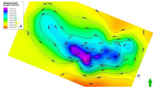
Figure 1.
Structural map of the Basal limestone top. Vertical cross section line A–A’.
In order to generate a basic parametric model of the structure, well survey data were used that included: geophysical log profiles, core sample measurements, well test results, etc. Those data resulted in lithological, stratigraphic, and geophysical detailed structures for all tested wells. In order to generate spatial distributions of basic geological parameters (porosity, permeability, net-to-gross ratio [NTG]), a 3D variographic analysis was performed for each of those parameters.
Resulting anisotropic variogram coefficients (sill, range values along main directions) together with parameter values determined at well positions were input parameters to generate stochastic realizations of corresponding spatial distributions. The averaging of such realizations resulted in the final distributions constituting a parameter model of the structure. Figure 2 presents vertical distributions of the main parameters: porosity and permeability along A–A’ vertical cross section.
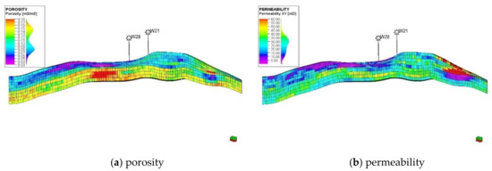
Figure 2.
Geological parameter distributions along the vertical cross section (A–A’).
3. Dynamic Simulation Model
3.1. Model Construction
The geological model was used as an input to construct the dynamic simulation model of the Borzęcin structure [15]. The model grid in its basic part consists of nine layers with their thickness varying between 5 and 13 m. Lateral sizes of the grid blocks equal to 80 × 80 m and enumerate up to 77 × 128 blocks. The 3D view of the model is shown in Figure 3. Its top view is shown in Figure 4. The cross section of the model structure is shown in Figure 5. The water–gas contact at the structure top defines reservoir contour and divide the model into the inner reservoir part and the outer surrounding aquifer part, as shown in Figure 6. In addition, the bottom layer of the model connects to underlying aquifers represented by analytical models of the Carter –Tracy type.
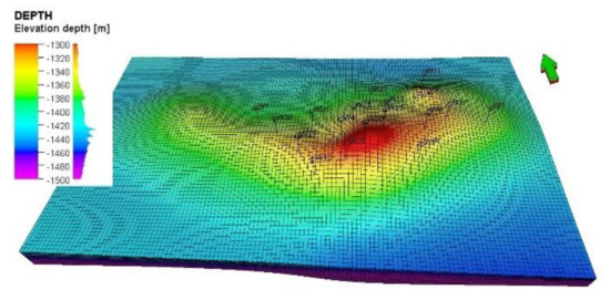
Figure 3.
3D view of the reservoir simulation model.
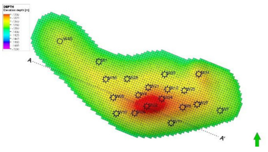
Figure 4.
Top view of the reservoir simulation model. Localization of additional well W40.
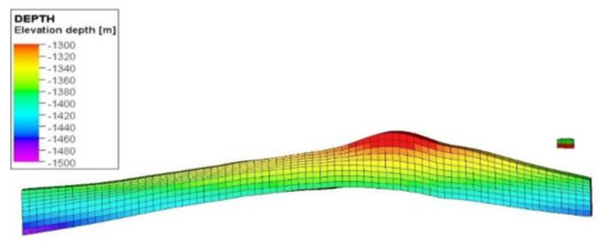
Figure 5.
Vertical cross section of the reservoir simulation model along line A–A’.
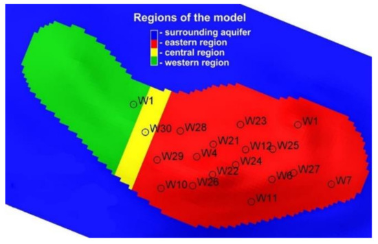
Figure 6.
Top view of the reservoir simulation model including surrounding aquifer. Definitions of partially isolated reservoir regions—see Section 3 for details.
Next, well data (well localizations, trajectories, diameters, completion intervals) were implemented into the model.
Model properties are supplemented with water saturation, Sw, and gas saturation, Sg = 1 − Sw, functions of capillary pressure, Pc, and relative permeabilities for water, krw, and gas, krg, in the water–gas system. The former was assumed of the following type (1, 2):
Parameters: end-point capillary pressure, Pa, power law exponent, λ, irreducible water saturation, Swir of these formula were determined to reconstruct (average) initial water saturation depth profiles measured in the wells of the reservoir as the functions of the height above the gas–water contact, and their values were found to be: Pa = 0.5 bar, λ = 0.1 in the Basal limestone, Pa = 0.5 bar, λ = 0.5 in the Rotliegend sandstone, Swir = 0.1.
The resultant initial gas saturation distribution in the reservoir was presented in Figure 7, Figure 8 and Figure 9 along A–A’ vertical cross section and at various layers of the model, respectively.
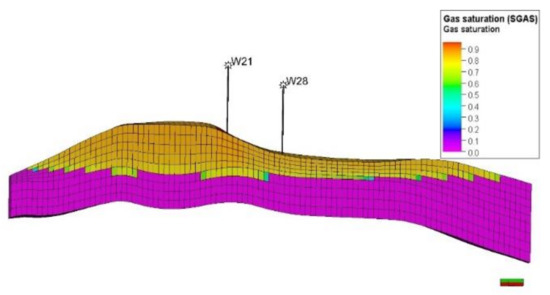
Figure 7.
Initial gas saturation along vertical cross section (A–A’).
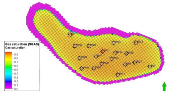
Figure 8.
Initial gas saturation at the Basal limestone top.
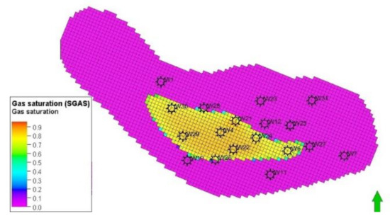
Figure 9.
Initial gas saturation at the Rotliegend top.
As no measurements were performed for relative permeabilities of samples from the Borzęcin structure, then their dependences of fluid saturations were assumed to be those of the neighbouring reservoirs located in the same formations [16]. They accept the following form (3, 4, 5):
with: α1 = 0.5 for the Basal limestone, α1 = 1.0 for the Rotliegend sandstone, α2 = −1, Sgr = 0.1.
In order to take into account varying composition of the gas within the structure and, consequently, its varying properties, a compositional model of the structure was constructed that adopted the Peng–Robinson equation of state. Six components (N2, CO2, H2S, C1, C2, C3+) of that gas were assumed with their standard equation of state (EOS) parameters. The composition of original gas is presented in Table 1. Viscosity properties of the gas were given by the standard Lorentz–Bray–Clark model. All the basic properties of the gas with varying composition under reservoir conditions were determined using the above EOS and viscosity model.

Table 1.
Composition of original fluid (gas) in the Borzęcin reservoir.
Assumed reservoir brine properties from the obtained data are: density: ρw = 1100 kg/m3, salinity: s = 150 g/l, formation volume factor: Bw = 1.011 Rm3/Sm3 @ P = 154.8 bar, T = 46.8 °C, compressibility: cw = 4.5 × 10⁻⁵ 1/bar, viscosity: µw = 0.66 cP, @ P = 154.8 bar, T = 46.8 °C, and viscosibility: 1/µw dµw/dp = 6 × 10⁻⁵ 1/bar.
In order to take into account effects of CO2 and H2S solubility in the reservoir brine, appropriate dependences of those solubilities upon varying reservoir pressures at the reservoir temperature were determined based on the laboratory measurements [17]. The measurement results were found to be best matched by the power-like correlations of CO2/H2S solubility, RS (CO2/H2S) vs. pressure, P (6):
as shown in Figure 10 and Figure 11 for CO2 and H2S, respectively. Here, the coefficients a0, a1, a2 were found to be: a0 = −0.5604/−1.1126, a1 = 1.1871/1.1871, a2 = −0.2685/−0.2685 for CO2/H2S, respectively.
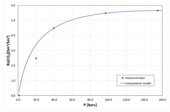
Figure 10.
Solution of CO2 in reservoir brine under reservoir conditions vs. pressure.
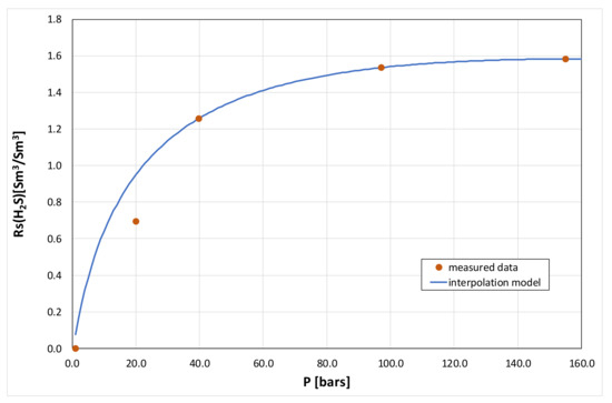
Figure 11.
Solution of H2S in reservoir brine under reservoir conditions vs. pressure.
3.2. Model Calibration
The simulation model of the Borzęcin structure of which construction was described above was subsequently calibrated against the complete set of the gas reservoir operational data [18]. The Borzęcin project operation includes two phases:
- production phase (1972–1995): production of the original natural gas,
- injection phase (1996–present): continuation of the gas production concomitant with acid gas reinjection.
The data of the production phase include gas and water production rates by all the active wells and regular bottom-hole pressures of those wells. The data of the injection phase include the amount (Figure 12) and composition (Figure 13) of the injected gas and composition of the produced gas (Figure 14) with varying contribution of the injecting gas components (CO2, H2S) in addition to the conventional data of the production wells (Figure 15 and Figure 16).
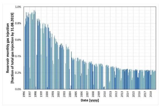
Figure 12.
Reservoir monthly gas injection. Fraction of total gas injection by 31.08.2019.
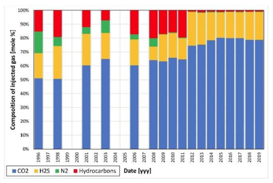
Figure 13.
Composition of injected gas.
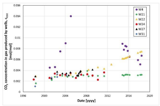
Figure 14.
CO2 concentration, CCO2, in gas produced by wells: W4, W21, W22, W24, W27, W31.
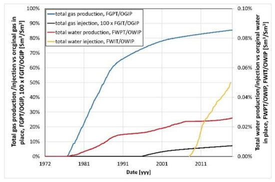
Figure 15.
Total gas production/injection relative to original gas in place. Total water production/injection relative to original water in place.
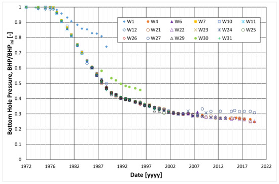
Figure 16.
Bottom-hole pressure of producing wells. Three trends identified as indicated by: (1). W1, (2). W30, (3). The other wells: W4, W6, W7, W10–W12, W21–W27, W29, W31.
The exemplary results of the calibration process for selected well W4 are given in: Figure 17, Figure 18 and Figure 19 for bottom-hole pressures, water–gas ratios, and CO2 concentrations of the produced gas, respectively.
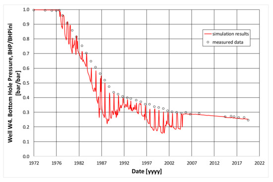
Figure 17.
Model calibration. Comparison of measured bottom-hole pressure and simulation results. Well W4.
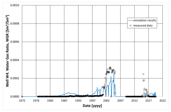
Figure 18.
Model calibration. Comparison of measured water–gas ratio and simulation results. Well W4.
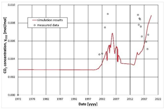
Figure 19.
Model calibration. Comparison of measured CO2 concentration and simulation results in gas produced by well W4.
The calibration process concluded with satisfactory match of the model results to the measured data. In order to obtain this match, several modifications of model parameters were introduced. The main modification divided the model into three partially separated regions (western, central, and eastern ones), as shown in Figure 6. This division was necessary due to three different measured pressure trends, as can be seen in Figure 16. As no faults, macro-fractures, or other structure barriers were recognized in the structural geological setting; lithological barriers were assumed to separate the regions. In order to precisely match the pressure trends in this regions, transmissibility properties of those barriers were determined by multiplying original transmissibility values by the factor of 0.01/0.5 for the barrier between western–central/central–eastern regions, respectively. Effective pore volumes of those regions were modified by the factor of 0.75/0.80 for the western/central region, respectively.
Other global parameters of the model, that were determined in the calibration process, include characteristic parameters (Time constant, Tc, Influx constant, β) of the analytical Carter–Tracy models of aquifers underlying three previously identified regions of the reservoir. Values of these parameters are given in Table 2.
Table 2.
Parameters of aquifer models.
The global vertical to horizontal permeability anisotropy was found to be kz/kx,y = 0.1 with the exceptions given in Table 3 where modifications of local transport properties in several well drainage zones, as found in the calibration process, are presented.
Table 3.
Modifications of model parameters from the calibration process.
4. Analysis of Simulation Results—Detailed Description of the On-Going Sequestration Process
4.1. Process Basic Parameters
The calibrated model of the Borzęcin structure is used for the detailed analysis of processes taking place during the sequestration project. Basic analysis refers to the pore pressure evolution within the Borzęcin structure. As indicated above in Section 3, three partially separated regions are identified within the Borzęcin structure. Average pressures of those regions significantly decline (as shown in Figure 20), and presently, they assume a small fraction of the initial value.
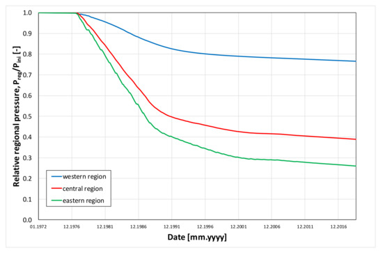
Figure 20.
Evolution of relative average regional pressures.
These reductions take place despite the behaviour of the surrounding and underlying aquifers. The amount of total water encroachment is minor compared to the original water in place (see Figure 21 and Figure 22), yet it cannot be neglected, as it is relevant when considering the pressure and water-to-gas ratio reconstructions of the producing wells.
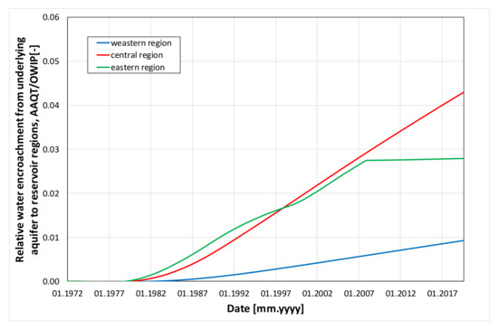
Figure 21.
Relative water encroachment from underlying aquifer to reservoir regions.
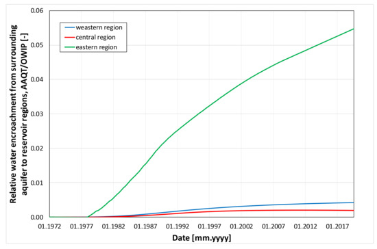
Figure 22.
Relative water encroachment from surrounding aquifer to reservoir regions.
Detailed pressure distributions within the structure volume are shown in Figure 23, Figure 24 and Figure 25 along the vertical cross section, at the structure top and bottom, respectively.
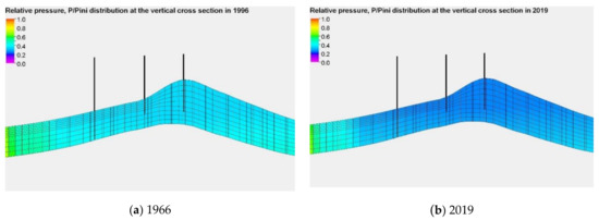
Figure 23.
Relative pressure distribution along the vertical cross section connecting wells: W29, W22, W11.
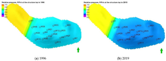
Figure 24.
Relative pressure distribution at the structure top.
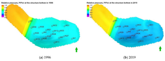
Figure 25.
Relative pressure distribution at the structure bottom.
A local maximum pressure is observed along the completion interval of the injecting well W28. Its time evolution is shown in Figure 26 for all layers of the well completion. That pressure does not exceed 40% of the reservoir initial pressure.
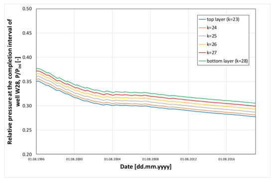
Figure 26.
Relative pressure at the completion interval of well W28.
Other interesting results of the simulations concern the reservoir fluid migrations and consequent mechanisms of CO2 trapping. Figure 27 shows the contributions of various trapping mechanisms—structural trapping related to the mobile CO2 gas phase, capillary trapping related to the immobile CO2 gas phase, solution trapping related to the CO2 aqueous phase—to the total sequestration process.
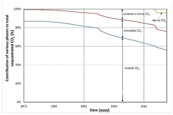
Figure 27.
Contribution of various phases to total CO2 in reservoir.
4.2. Leakage Risk Factor Analysis
The simulation results presented in the above section were used to analyse various gas leakage [19] risk factors. The maximum pressure is compared with the formation breakdown (fracturing) pressure, Pbd [20], as calculated from the geomechanical model simulations [21]. The calculated breakdown pressure distribution within the Borzęcin structure is shown in Figure 28. The maximum pore pressure during the injection phase of the acid gas sequestration project is much lower than the formation breakdown pressure. Consequently, there is no risk of any induced fractures to be generated and no leakage risk due to fracture pathways.
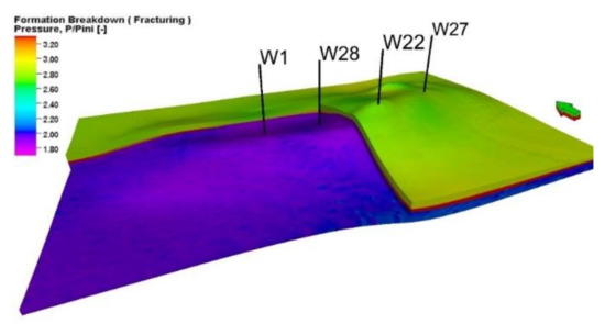
Figure 28.
Distribution of the formation breakdown pressure within the Borzęcin structure.
Another potential leakage pathway may occur through the caprock above the reservoir rock. Its sealing properties are, first of all, determined by threshold displacement pressure [22,23]. This pressure for the Borzęcin structure can be estimated by analysing initial pressure profile across gas zone vs. hydrostatic pressure profile in the caprock at the highest point of the caprock–reservoir rock boundary and by taking into account the complete sealing properties of the caprock under those conditions. This pressure profile is shown in Figure 29, and the lower limit of the threshold displacement pressure is found to be 9.2 bars.
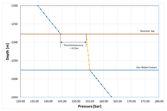
Figure 29.
Diagram for the estimation of the threshold displacement pressure at the caprock–reservoir rock boundary under initial conditions.
As the maximum pressure at the structure caprock–reservoir rock boundary is much reduced compared to the initial pressure, the pressure step across the boundary never exceeds the estimated threshold displacement pressure. Consequently, there is no leakage risk due to pathways developed in the caprock.
Another significant characteristic of the acid gas sequestration project is the extension of the gas plume containing the injected acid gases [24]. As the acid gases are injected into the water-bearing zone, their presence in the water phase also requires closer examination. The distributions of relevant quantities are shown in Figure 30, Figure 31, Figure 32 and Figure 33 for gas saturation, CO2 concentration in the gas phase, brine saturation, and CO2 solution in the brine phase, respectively.
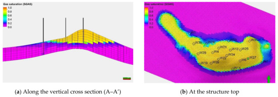
Figure 30.
Distribution of gas saturation in 2019.
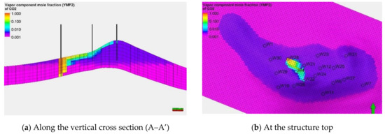
Figure 31.
Distribution of CO2 concentration in the gas phase in 2019.
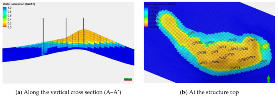
Figure 32.
Distribution of brine saturation in 2019.
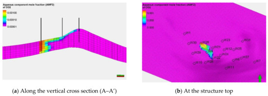
Figure 33.
Distribution of CO2 solution in brine (immobile at Sw < 0.1, mobile otherwise) in 2019.
As seen in the above figures, the extension of the gas plume containing CO2 as well as the CO2 dissolved in the brine are confined within the initial gas cap extension (Figure 8) being the original reservoir contour. Consequently, there is no leakage risk due to either gas containing CO2 or brine with dissolved CO2 to spill out beyond the structural trap of the Borzęcin structure.
These results also follow the basic phenomena of multiphase flow of reservoir fluids including buoyance effects, as can be observed in Figure 30, Figure 31, Figure 32 and Figure 33 vs. Figure 9 and Figure 10.
Another potential leakage risk is related to the variation of geomechanical status along the existing wells and, consequently, the bond of the cement to reservoir rock and well casing. This issue will be the subject of a separate publication concerning geomechanical model of the Borzęcin structure [21].
To summarise, in the analysed case of the Borzęcin project, results of its simulation modelling clearly show no leakage risk—a conclusion consistent with the monitoring results [17]. However, in general, it should be emphasized that lack of measuring evidences during the project operation is not a sufficient condition for leakage-free sequestration process. This is caused by typically prolonged migration processes of the gas to leak upwards all the way from the sequestration site to the surface, where it can be detected. Therefore, the long-term simulation modelling of sequestration projects proves to be a unique method for the quantitative leakage risk analysis. An example of such long-term simulations is presented in the next section.
5. Storage Capacity Analysis for a Full-Scale CO2 Sequestration Scenario at Borzęcin
5.1. Simulation Forecast Assumptions
At present, the reservoir properties of the Borzęcin structure are characterized by the following:
- –
- the amount of gas in place is reduced to 85% of the original gas in place (Figure 15),
- –
- the average reservoir pressure is also significantly reduced, in particular, it reaches less than 30% of the initial pressure in the dominant eastern region of the structure (Figure 20),
- –
- most of the producing wells can be converted to injection wells at relatively low cost,
- –
- in addition, other elements of the existing surface installation can be converted for the purposes of an alternative sequestration project.
All the above points suggest that the Borzęcin facility can be considered as a potential site of a large-scale CO2 sequestration project. In the following, reservoir characteristics of such a project are presented as the results of simulation studies including estimation of the structure sequestration capacity [25,26].
The existing system of wells does not cover the whole area of the Borzęcin reservoir. In particular, the western region of the reservoir does not include any operating well. Therefore, one additional well (W40) is assumed to complete the existing system of wells in the location shown in Figure 4.
As a result, 17 wells (W4, W6, W7, W10, W11, W12, W21, W23, W22, W24, W25, W26, W27, W28, W29, W30, W31) cover the eastern region, a single well (W30) covers the central regions, and two wells (W1, W40) cover the western region.
All the wells are assumed to be completed in the water-bearing layers below the gas cap. The nominal, maximum injection rate is set at 400,000 Sm3/d, and the bottom-hole injection pressure is limited to 200 bars—the value consistent with the formation breakdown pressure.
Multiple scenarios of the CO2 injection project were performed with the calibrated model of the Borzęcin structure and tested against the following risk determining factors:
- –
- no spill-out of the injected CO2 beyond the structural trap,
- –
- maximum pressure in the structure volume below the fracturing pressure,
- –
- maximum pressure step across the caprock–reservoir rock boundary below the threshold displacement pressure.
It should be noted that all the above factors are directly dependent upon the degree of the structure filling with the sequestrated gas and, thus, uniquely determine its capacity. Another leakages risk factor—deteriorated well integrity—is not studied here. Its influence upon the structure sequestration capacity is more complex and depends on various factors not necessarily related to the overall project characteristics.
The optimum scenario that fulfils the above criteria and maximizes the injected CO2 amount was calculated. The characteristics of the optimum scenario are presented below.
5.2. Simulation Forecast Results and Analysis
The injection time interval lasts for 113 months (from January 2020 until May 2029). Then the simulation forecast is extended for the next one hundred years of relaxation the total injection rate is constant for 96 months of the gas injection (from January 2020 until December 2027) and is slightly reduced afterwards while most of the injected CO2 moves to the eastern region of the structure (Figure 34). The total volume of the injected CO2 exceeds that of the original gas in place (OGIP) and amounts to 135% of OGIP (Figure 35). The average sequestration capacity coefficients are found to be: 53.20 kg of gaseous CO2 per 1 m3 of pore volume saturated with gas and 3.54 kg of dissolved CO2 per 1 m3 of pore volume saturated with brine. The analysis of various trapping mechanisms [27] results in the following: most of the sequestrated CO2 (79%) becomes a mobile gas, approximately 20% is in the immobile gas saturation, and the rest is dissolved in the reservoir brine (Figure 36).
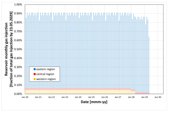
Figure 34.
Regional monthly CO2 injection.
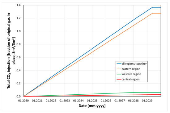
Figure 35.
Evolution of total CO2 injection.
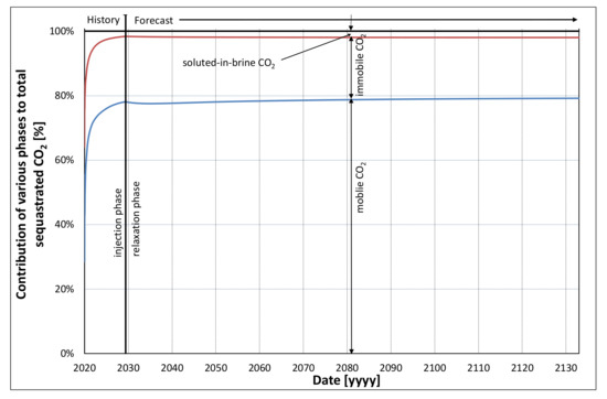
Figure 36.
Contribution of trapping mechanisms to the total sequestration.
The average reservoir pressures in the three structure regions significantly increase during the injection phase of the project and slightly decline during the relaxation phase (Figure 37). This pressure behaviour results not only from the injection schedule but also from the aquifer activities. During the sequestration project the reservoir water is pushed back to the aquifers (Figure 38 and Figure 39), and this process effectively increases the reservoir volume available to the injected CO2. The maximum pressure in the structure volume is observed at the end of the injection phase. Its values at that time are presented in Figure 40. The maximum local pressure is found along the injecting well trajectories, and its absolute maximum amounts to 108% of the initial reservoir pressure (Figure 41). This value is much below the formation breakdown pressure of the corresponding reservoir rock (Figure 28). Hence, there is no risk of the gas leakage via a fracture pathway as required for the leakage-free sequestration project.
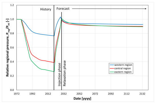
Figure 37.
Average reservoir pressure.
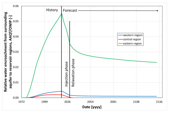
Figure 38.
Relative water encroachment from surrounding aquifer to reservoir regions.
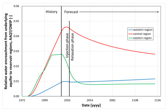
Figure 39.
Relative water encroachment from underlying aquifer to reservoir regions.
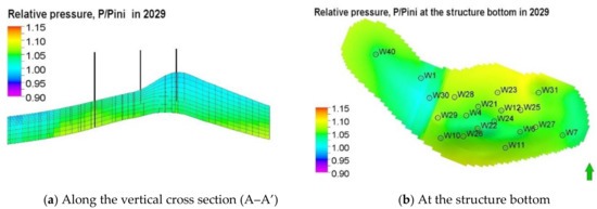
Figure 40.
Reservoir pressure distribution at the end of the injection phase (2029).
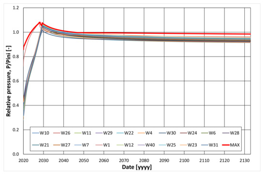
Figure 41.
Maximum pressures along well trajectories. Maximum pressures among all well trajectories.
The next factor of the leakage risk refers to the pressure step across the caprock–reservoir rock boundary. That step, as a function of time, reaches its maximum value at the end of the injection phase (2029). The distribution of the step pressure at that time is shown in Figure 42. The maximum value of the step takes place in the neighbourhood of W22, which is the highest structure point, and its evolution with time is shown in Figure 43.
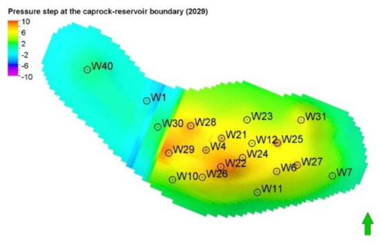
Figure 42.
Distribution of pressure step across the caprock–reservoir rock boundary in 2029.
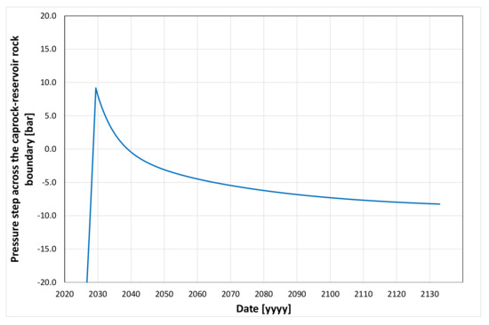
Figure 43.
Pressure step across the caprock–reservoir rock boundary at the high structure point.
Hence, the criterion of the pressure step across the caprock–reservoir rock boundary not exceeding the threshold displacement pressure (9.2 bars in Figure 29) is fulfilled. This is relevant, as it is among the risk factors that effectively limits the amount of the injected CO2 and, hence, determines the sequestration capacity of the structure.
Another important factor to ensure the effectiveness of the sequestration process is the extension of the injected gas plume [24] that should fill out the structural trap to the maximum degree and avoid the injected gas spill-out beyond the trap. The same comment applies to the brine with the dissolved gas. In addition, the homogeneity of the injected gas distribution across the structure volume guarantees the maximum of the sequestration capacity. The corresponding results of the significant parameters for the analysed case are shown in the following figures:
- –
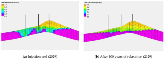 Figure 44. Distribution of gas saturation along the vertical cross section (A–A’).
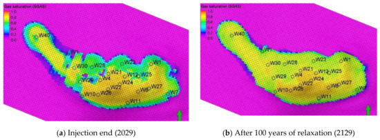 Figure 45. Distribution of gas saturation at the structure top.
- –
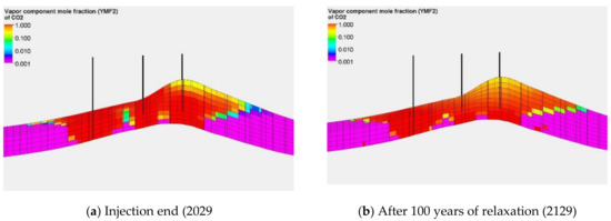 Figure 46. Distribution of CO2 concentration in the gas phase along the vertical cross section (A–A’).
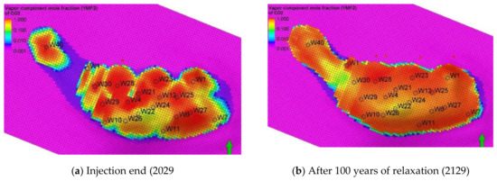 Figure 47. Distribution of CO2 concentration in the gas phase at the structure top.
- –
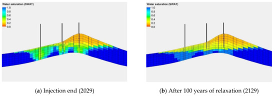 Figure 48. Distribution of brine saturation along the vertical cross section (A–A’).
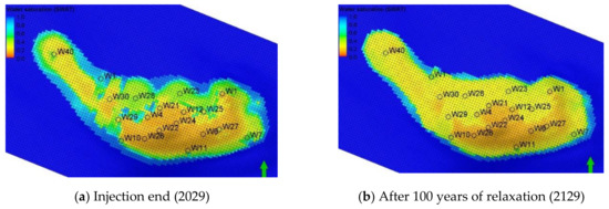 Figure 49. Distribution of brine saturation at the structure top.
- –
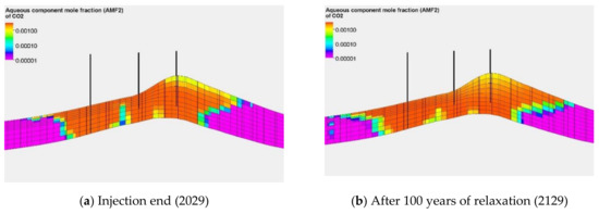 Figure 50. Distribution of CO2 solution in brine along the vertical cross section (A–A’).
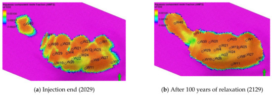 Figure 51. Distribution of CO2 solution in brine at the structure top.
It should be noted that in order to determine the key parameters of the sequestration process, it is required to extend the examination of the project beyond the end of the injection phase. This allows for the elongated relaxation phase that typically results in redistribution of fluid saturations and compositions as well as reservoir pressure variation to be included in modelling.
The scenario presented above maximizes the sequestration capacity of the structure while maintaining a leakage-free operation of the sequestration process. The scenario of maximum sequestration capacity is a result of the optimization procedure using multiple simulation forecasts. Capability of performing the optimization procedure proves to be another significant advantage of the numerical modelling tool applied to the sequestration project assessment.
6. Summary and Conclusions
This paper presents a study on the quantitative description and analysis of the acid gas (CO2 and H2S) sequestration in a deep geological structure, where the gas is injected to the water-bearing zone underlying the natural gas reservoir. The study employs a 3D, compositional reservoir model of the structure that includes all the significant mechanisms taking place during the sequestration process: multiphase flow of reservoir fluids, buoyance effects, gas dissolution in reservoir water, gas trapping by capillary forces.
Due to the large set of operational and monitoring data acquired during 24 years of continuous project operation, the model undergoes a detailed calibration procedure and provides reliable results of reservoir fluid migration, redistribution of their saturations and compositions, as well as pore pressure distributions at various stages of project advancement. These results are also input data to assess various risk factors of the stored gas leakage, in particular, leakage due to injected gas spill-out beyond the structural trap, leakage along induced fractures, or leakage through the caprock.
Although the monitoring data provide hard and direct information about leakage presence or absence, these data are limited by their space extent and, obviously, to the past and present time. However, it should be emphasized that lack of measuring evidences during the project operation is not a sufficient condition for leakage-free sequestration process. This is caused by typically prolonged migration processes of the gas to leak upwards all the way from the sequestration site to the surface where it can be detected. Therefore, the long-term simulation modelling of sequestration projects proves to be a unique method for the complete leakage risk analysis.
Another advantage of a reliable model of the sequestration process is its capability to assess the future consequences of the sequestration project and to make their analyses. It should be emphasized that the forecast should include a long-time relaxation period extending beyond the injection schedule of the project. During the relaxation period, a significant redistribution of pressures and fluid saturations may occur and usually does occur, which affects leakage risk factors. Therefore, performing project simulation forecasts comprising relaxation period of sufficient duration is a key requirement for a thorough analysis of the sequestration project. Again, the application of the project numerical modelling proved to be a necessary tool of the project assessment. All the above points as referred to the analysed case were discussed in the paper.
In addition, the reservoir model of the case was applied to determine the maximum sequestration capacity of the structure while maintaining a leakage risk-free operation of the sequestration process. The scenario of maximum sequestration capacity was found as a result of the optimization procedure using multiple simulation forecasts. Capability of performing the optimization procedure proved to be another significant advantage of the numerical modelling tool applied to the sequestration project assessment.
Author Contributions
Conceptualization, W.S.; methodology, A.G. and P.Ł.; software, K.M.; validation, W.S.; formal analysis, W.S.; investigation, A.G., P.Ł. and K.M.; resources, A.G. and K.M.; data curation, P.Ł. and K.M.; writing—original draft preparation, W.S.; writing—review and editing, W.S.; visualization, A.G. and K.M.; supervision, W.S.; project administration, W.S. All authors have read and agreed to the published version of the manuscript.
Funding
This report is part of a project that has received funding by the European Union’s Horizon 2020 research and innovation programme under grant agreement number 764531. Project acronym and title: SECURe—Subsurface Evaluation of Carbon capture and storage and Unconventional Risks. D2.2 Report on effects of long-term sequestration process in the Borzęcin structure—observation evidence of the injected gas migration and possible leakage.
Conflicts of Interest
The authors declare no conflict of interest.
References
- Lubaś, J.; Szott, W. 15-year experience of acid gas storage in the natural gas structure of Borzęcin—Poland. Nafta-Gaz 2010, 66, 333–338. [Google Scholar]
- In Salah Fact Sheet: Carbon Dioxide Capture and Storage Project. Available online: https://sequestration.mit.edu/tools/projects/in_salah.html (accessed on 14 March 2020).
- GDF K12-B Offshore CO2 Injection Project. Available online: https://www.co2-cato.org/cato/locations/regions/western-netherlands/gdf-k12-b-offshore-co2-injection-project (accessed on 14 March 2020).
- Akervoll, I.; Lindeberg, E.; Lackner, A. Feasibility of Reproduction of Stored CO2 from the Utsira Formation at the Sleipner Gas Field. Energy Procedia 2009, 1, 2557–2564. [Google Scholar] [CrossRef]
- Weyburn-Midale. The IEAGHG Weyburn-Midale CO2 Monitoring and Storage Project. Available online: https://ptrc.ca/projects/past-projects/weyburn-midale (accessed on 14 March 2020).
- Read, A.; Onno, T.; Menno, R.; Jonker, T.; Hylkema, H. Update on the ROAD Project and Lessons Learnt. Energy Procedia 2014, 63, 6079–6095. [Google Scholar] [CrossRef]
- Estubliera, A.; Lacknerb, A.S. Long-term simulation of the Snøhvit CO2 storage. Energy Procedia 2009, 1, 3221–3228. [Google Scholar] [CrossRef]
- Lubaś, J.; Szott, W.; Jakubowicz, P. Effects of Acid Gas Reinjection on CO2 Concentration in Natural Gas Produced from Borzęcin Reservoir. Nafta-Gaz 2012, 68, 405–410. [Google Scholar]
- Van der Meer, L.G.H. Computer modelling of underground CO storage. Energy Convers. Manag. 1996, 37, 1155–1160. [Google Scholar] [CrossRef]
- Jiang, X.; Akber Hassan, W.A.; Gluyas, J. Modelling and monitoring of geological carbon storage: A perspective on cross-validation. Appl. Energy 2013, 112, 784–792. [Google Scholar] [CrossRef]
- Agarwal, R.K. Modeling, Simulation, and Optimization of Geological Sequestration of CO2. ASME J. Fluids Eng. 2019, 141, 100801. [Google Scholar] [CrossRef]
- Soltanian, M.R. Multicomponent reactive transport of carbon dioxide in fluvial heterogeneous aquifers. J. Nat. Gas Sci. Eng. 2019, 65, 212–223. [Google Scholar] [CrossRef]
- Gershenzon, N.I. Influence of small-scale fluvial architecture on CO2 trapping processes in deep brine reservoirs. Water Resour. Res. 2015, 51, 8240–8256. [Google Scholar] [CrossRef]
- Polish Oil and Gas Company. Geological Documentation of the Borzęcin Natural Gas Reservoir, 1999. Personal communication, 2019. [Google Scholar]
- Szott, W.; Gołąbek, A.; Miłek, K. Symulacyjne badanie procesów sekwestracji gazów kwaśnych w wodach podścielających złoża naftowe (Simulation studies of acid gas sequestration in aquifers underlying gas reservoirs). Pr. Inst. Naft. I Gazu 2009, 165, 1–89. [Google Scholar]
- Szott, W.; Łętkowski, P.; Gołąbek, A.; Miłek, K. Ocena efektów wspomaganego wydobycia ropy naftowej i gazu ziemnego z wybranych złóż krajowych z zastosowaniem zatłaczania CO2 (Assessment of EOR/EGR processes by CO2 injection for selected Polish oil and gas reservoirs). Pr. Nauk. Inst. Naft. I Gazu 2012, 184, 1–161. [Google Scholar]
- Warnecki, M.; Wojnicki, M. Monitoring of acid gas migration in the Borzęcin structure. Unpublished Work.
- Polish Oil and Gas Company. Historical production data of the Borzęcin reservoir—reported by Polish Oil and Gas Company (POGC)—various reports in free format 1972–2019. Personal communication, 2019. [Google Scholar]
- Mortezaei, K.; Amirlatifi, A.; Ghazanfari, E.; Vahedifard, F. Potential CO2 Leakage from Geological Storage Sites: Advances and Challenges. J. Environ. Geotech. 2018. [Google Scholar] [CrossRef]
- Jin, X.; Shah, S.N.; Roegiers, J.-C.; Hou, B. Breakdown Pressure Determination—A Fracture Mechanics Approach. In Proceedings of the SPE Annual Technical Conference and Exhibition, New Orleans, LA, USA, 30 September–2 October 2013. SPE 166434. [Google Scholar]
- Szott, W.; Słota-Valim, M.; Gołąbek, A.; Łętkowski, P. Geomechanical modelling of the Borzęcin structure. Unpublished Work.
- Thomas, L.K.; Katz, D.L.; Tek, M.R. Threshold Pressure Phenomena in Porous Media. Soc. Pet. Eng. J. 2013, 8, 174–184. [Google Scholar] [CrossRef]
- Farokhpoora, R.; Akervolb, I.; Torsætera, O.; Bjørkvikb, B.J.A. CO2 capillary entry pressure into flow barrier and caprock. In Proceedings of the International Symposium of the Society of Core Analysts, Napa Valley, CA, USA, 2013, 16–19 September; pp. 1–8.
- Bhowmik, S.; Srinivasan, S.; Bryant, S.L. Predicting the Migration of CO2 Plume Using Injection Data and a Distance-Metric Approach to Reservoir-Model Selection. Soc. Pet. Eng. 2010. [Google Scholar] [CrossRef]
- Bachu, S.; Bonijoly, D.; Bradshaw, J.; Burruss, R.; Holloway, S.; Christensen, N.P.; Mathiassen, O.M. CO2 storage capacity estimation: Methodology and gaps. Int. J. Greenh. Gas. Control. 2007, 1, 430–443. [Google Scholar] [CrossRef]
- Kopp, A.; Probst, P.; Class, H.; Hurter, S.; Helmig, R. Estimation of CO2 Storage Capacity Coefficients in Geologic Formations. Energy Procedia 2009, 1, 2863–2870. [Google Scholar] [CrossRef]
- Suekane, T.; Nobuso, T.; Hirai, S.; Kiyota, M. Geological storage of carbon dioxide by residual gas and solubility trapping. Int. J. Greenh. Gas. Control. 2008, 2, 58–64. [Google Scholar] [CrossRef]


© 2020 by the authors. Licensee MDPI, Basel, Switzerland. This article is an open access article distributed under the terms and conditions of the Creative Commons Attribution (CC BY) license (http://creativecommons.org/licenses/by/4.0/).