Abstract
High variable renewable energy (VRE) penetration led to the first-ever VRE curtailment in Japan, occurring in Kyushu in October 2018. Since then, there has been an average of 3% solar curtailment, with a peak of 13.7% in April 2019, resulting in approximately ¥9.6 billion of wasted energy. The VRE curtailment is expected to worsen as VRE penetration continues to increase along with nuclear energy increment in line with Japan’s 2030 energy goals. To prevent this curtailment and increase energy stability, a novel, logic-based forecasting method using hourly supply/demand data was developed. Initially, inaccurate results were returned; however, after several rounds of calibration that adjusted the quartile value of the max/min operating windows, the overall accuracy of this method was increased to 97% of real curtailment. This calibrated model was then used to test several curtailment mitigation scenarios. Some scenarios increased curtailment, while the two most successful scenarios, which reduced the installed nuclear capacity either seasonally or totally, limited curtailment by 95% and 97%, respectively. Another scenario with increased grid interconnection between regions reduced curtailment by 79%. Moreover, it would provide other benefits by unifying the national grid thereby increasing disaster resistance, reducing curtailment, improving grid flexibility and allowing for higher VRE penetrations. Currently, the situation is worsening, and some actions are required to reduce the curtailment and to achieve its 2030 energy goals in Japan. The mitigation measures studied by the logic method could be recommended to be referred to.
1. Introduction
The energy sector in Japan has changed dramatically since the 2011 Fukushima Daiichi nuclear disaster, with a substantial increase in solar photovoltaic (PV) penetration due to a high feed-in tariff (FIT) introduced in Japan in 2012 [1]. The FIT incentivizes private developers to build solar PV systems across the country and sell their electricity to local power companies. Some regions, namely, Kyushu and Hokkaido, have seen higher development of solar PV due to low land cost than the rest of Japan. This very high growth rate is good for the energy self-sufficiency of Japan, which has been decreasing since the Fukushima disaster, and for the environment [2].
One of the main challenges that variable renewable energy (VRE) presents is that it is “variable” and “non-controllable”, meaning that VRE output cannot be controlled by the utilities and that its output can vary widely minute by minute. Since the utilities have to ensure a balance between supply and demand at all times, this variable supply can cause a problem. Therefore, if a large amount of a variable source of electricity such as solar energy is introduced without implementing any type of demand management, energy storage or energy sharing across regions, then there is a risk of VRE curtailment. Curtailment is therefore defined as the act of restricting or reducing the energy supply from a generator to the electrical grid. It can be classified as a type of inefficiency as not all the energy that is produced, is used. While curtailment can be useful to ensure energy balance, reducing the curtailment and thereby improving the system efficiency should be the goal of utility companies.
1.1. Curtailment in Japan
High levels of planned VRE, such as in Japan’s 2030 goals, require some modifications to the existing infrastructure as well as changes to energy policies to accommodate the high VRE and thereby avoid curtailment [3]. These actions have yet to be taken in Japan. While the overall VRE penetration in Japan was still quite low as of 2019, the VRE penetration in the Kyushu Prefecture of Japan was much higher, accounting for up to 47% of the energy supply [4]. This, along with the reestablishment of constant nuclear energy in the region, has added extra pressure on the utility company (Kyuden) to maintain the energy balance [5], leading to the first-ever VRE curtailment in Japan occurring in Kyushu in October 2018. Since then, there has been an average of 3% solar curtailment in Kyushu, with a peak of 13.7% in April 2019 [6], resulting in approximately ¥9.6 billion of wasted energy as of September 2019 [7].
VRE curtailment had never occurred before 2018 in Japan. However, there is a provision for it in the FIT agreement, which states that grid operators can enforce curtailment against renewable electricity producers without compensation up to 30 days per facility per year to balance supply and demand; grid operators are obliged to compensate for curtailment over 30 days. Grid operators can also refuse connection agreements when curtailment is anticipated to go over 30 days [1].
Worsening the curtailment situation is the design of the Japanese grid connections between regions. The electricity grid and companies in Japan are divided into ten regions (Figure 1). Each region acts mostly independently of each other, and therefore, the inter-grid connections only allow a limited amount of electricity transfer between regions [4]. In the case of Kyushu, the grid is only connected to that of one neighbouring region, namely, Chugoku, through the Kanmon Interconnection line [8]. This connection is saturated, as the scheduled power flow (SPF) is almost always at the total transfer capability (TTC). This means that when curtailment is about to occur, there is not much capacity left in the inter-grid connection. Furthermore, as of 2016, there was no planned development of the Kanmon Interconnection line [9].
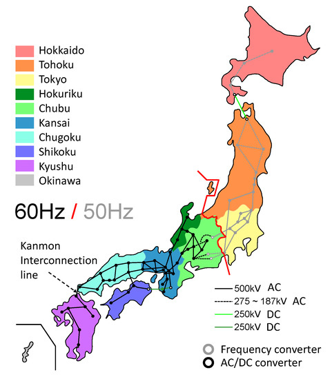
Figure 1.
Electricity grid and utilities in Japan (Source: Callum, 2013).
1.2. Worldwide Curtailment
The problem of curtailment is increasing worldwide as VRE penetration grows [3], and several countries around the world have experienced VRE curtailment. Table 1 shows the most recently available data as of March 2020. Several countries are compared based on a metric called the curtailment (C) and penetration (P) ratio (CP ratio) [10]. The CP ratio shows the correlation between the solar and wind energy curtailment and the solar and wind energy produced in relation to the overall energy demand. This helps quantify and compare different regions to each other, even though the countries have very different VRE situations.

Table 1.
Statistical data for several countries and regions and the resulting curtailment classification.
Based on the CP ratio, each country can be classified on its current (latest) situation using three colours, namely, red, yellow and green. In addition, the CP gradient shows the current (latest) trend of the curtailment using three classifiers: deteriorating, stable and improving [10]. From this, the following summaries can be drawn. VRE curtailment in Japan is very low, even as of 2019, when curtailment was at only 0.47%, leading to a classification of green and stable. However, the situation in Kyushu is very different from that in the rest of the country. A large increase in curtailment from 2018 to 2019 from 0.22% to 3.01% led to a classification of yellow and deteriorating. This indicates that the curtailment in Kyushu is worsening, which is in line with the analysis performed in 2015 [10].
Interestingly, the CP ratio observed in 2019 in Kyushu is the fourth largest of the regions analysed, with China having the largest ratio, followed by that of Italy and Europe 28. One distinction that has to be made, however, is that all the other countries encountered curtailment before 2018 and have therefore had time to improve their curtailment mitigation techniques. However, curtailment in Kyushu just started in 2018 and may continue to worsen before Kyuden can mitigate it, if Kyuden chooses to do anything. Another interesting note is that only three regions have deteriorating curtailment classifications, namely, Kyushu, Ireland and China, with Ireland having the worst CP gradient, followed by Kyushu and China. These regions are currently suffering from increasing levels of curtailment. Last, it is beneficial to investigate the VRE penetration levels of the different countries. The levels in some European countries, such as Denmark, Spain and Germany, are significantly higher than those in Japan, the USA and China, making these countries more susceptible to curtailment. However, their CP ratios are relatively low, indicating that curtailment can be mitigated somewhat even with much higher levels of VRE penetration.
1.3. Mitigation of Curtailment
Mitigation techniques to reduce future curtailment needs to be addressed. This requires that curtailment be forecasted and then different mitigation scenarios be tested. However, there has been limited literature on curtailment forecasting, particularly forecasting with high temporal resolution, such as hour-by-hour forecasting. There are several examples of forecasting demand. Several simple models, such as time series and regression models, exist, with increasingly complex models using artificial neural networks or combinations of different models [20,21]. Some supply types can also be modelled using some of these methods together with future climate models. The problem occurs when modelling controllable supplies, i.e., supplies that are adjusted to maintain the supply-demand balance. However, no previous research reporting a model to forecast the hourly behaviour of these supply types was identified in this study. Calculating curtailment requires that all the supplies and demands in the system are known or calculated so that all surplus can be calculated. Therefore, in this research, a new model, called the logic model, was developed to calculate the controllable supplies and thereby the curtailment. In addition, since curtailment in Japan occurred recently in October 2018, there is little to no research about the recent curtailment situation in Japan. Therefore, this paper tries to address these shortcomings.
Mitigating VRE curtailment can be done in several ways in both policy and technological adjustments. The main technological adjustment that can be made is increasing the maximum and minimum operating limits of the existing supplies [5] or simply adjusting the amount of installed capacity of each existing type of generatio. Another technological adjustment is to improve the inter-grid electricity transfer. This is one main advantage that European countries have, as there is strong grid transfer between regions, whereas Japan has limited infrastructure for transferring electricity between different energy companies. Several other methods are to improve the next-day forecasting of VRE, allowing for better planning with other supplies. The introduction of negative bidding can incentivize independent power producers (IPPs) to not sell electricity at certain times and rather to store electricity or send it to other regions. Last, setting VRE ramp limits can incentivize IPPs to manage ramp rates or face penalties [3,5,22].
In this research, it is hypothesized that curtailment will worsen as VRE penetration continues to increase and as nuclear energy increases in line with Japan’s 2030 energy goals unless appropriate mitigation measures are taken immediately. Therefore, the objectives of this research are to understand the causes of curtailment in Kyushu, forecast future supply and demand, and then calculate curtailment. Finally, once the future curtailment is calculated, different scenario-based mitigation measures are evaluated based on cost-benefit analysis, and the best mitigation scenario is recommended.
The paper is organised as follows: Section 2 describes the materials and methodology used in this study. In the methodology section, we introduce a novel logic method in detail developed for this study to forecast the curtailment and present the forecast results of the logic method. The results and discussion about the mitigation techniques are given in Section 3 and Section 4, respectively, which are followed by the conclusions in Section 5.
2. Materials and Methodology
The overall methodology for curtailment prediction and mitigation technique testing is shown in Figure 2. The overall process is divided into four steps. Data preparation and pre-processing occur in the first two steps, the main forecasting is carried out in step 3 and mitigation technique testing is considered in step 4.
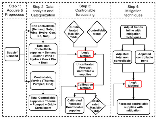
Figure 2.
Overall flowchart of the methodology with four steps.
2.1. Materials
2.1.1. Data and Pre-Processing
The main dataset used in this research is the hourly supply/demand breakdown for the Kyushu region in Japan from April 2016 to September 2019 from Kyuden in 3-month files [23] and from the Institute for Sustainable Energy Policies (ISEP) in yearly datasets [11]. The data contain time and date stamps, demand and all the supplies for each hour, all in MWh.
Figure 3 shows monthly average values of the stagnant demand, decreasing thermal supply, increasing nuclear and solar supply, and rapidly increasing curtailment starting from October 2018 in addition to the overall trends. The curtailment occurs in the off-peak seasons, autumn and spring, of demand when nuclear had reached a critical level. The increasing nuclear energy has a clear correlation to curtailment because as it increased, thermal energy decreases. Therefore, there is less flexibility in the energy supply allowing for potentially higher curtailment on days with excess VRE.
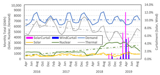
Figure 3.
Main factors influencing curtailment in Kyushu from April 2016 to September 2019.
Figure 4 shows the hourly variation in the supply and curtailment of the day with the highest curtailment, 7 April 2019, and is key to understanding the behaviour of all supplies when curtailment occurs. Before 5 am, there was no curtailment, and the demand was mostly met with nuclear and thermal energy. There was a constant value of grid interconnection energy being sent to the neighbouring Chugoku region, as well as a small amount of positive pumped storage energy, which indicates that the pumped storage was releasing energy at that time.
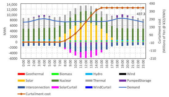
Figure 4.
Highest curtailment day in Kyushu, 7 April 2019, showing the supply and demand balance with curtailment cost.
Regarding the demand on 7 April 2019, it was a Sunday in spring, and therefore, the demand was quite low. Japan suffers from extreme heat and cold in the summer and winter, respectively, implying that electricity demand peaks at those times, with the troughs being in the spring and autumn.
At 6 am, solar generation began and ramped up quite quickly to its maximum at 12:00. This ramp-up was one of the largest causes of curtailment, as the other supplies could ramp down quickly enough to maintain the balance. As soon as solar generation starts, thermal generation is reduced because the thermal energy reduction is the main form of balancing the supply and demand. However, the thermal generation cannot decrease to zero. It has a minimum amount that it cannot go below. It also has a maximum hourly ramp-down rate that cannot be exceeded.
Table 2 summarizes the monthly solar curtailment between September 2018 and September 2019, and its estimated cost. The curtailment during this period was 2.7%, which is quite low compared to that of other countries. This is further reinforced by the monthly curtailment, where in October 2018, curtailment is only 1.3%. However, from February 2019 to April 2019, the monthly curtailment increased from 0.4% to 6.8% and then 12.1% in April. The curtailment was set to continue in May. The total value of all the curtailments was approx. ¥9.6 billion, with 98% of that coming from solar curtailment. This approximate curtailment cost was calculated using the average FIT tariff for 2012–2015 multiplied by the curtailed energy [7].
Table 2.
Monthly VRE generation and curtailment in MWh and curtailment cost.
2.1.2. Categorisation of Supplies
Figure 5 shows the energy generation sources in Kyushu for 2018 compared to the nationwide generation. Kyushu generated significantly more electricity from nuclear than the nation as a whole. Only three regions restarted nuclear energy generation in Japan post-2011, with Kansai and Kyushu having the highest energy generation. This is extremely significant to curtailment, as nuclear energy is “non-controllable” and “constant”, and it accounts for 21% of the total energy supplied in Kyushu in 2018. Along with this, solar generation was much higher as well. These are the two main factors affecting curtailment. Furthermore, Kyushu’s thermal generation was much lower than that nationwide, as the high nuclear generation required thermal to decrease; while this is good for the environment, it reduces one of the largest tools to mitigate curtailments. Geothermal in Kyushu was higher than that nationwide but only accounts for 1% of generation, whereas biomass was similar to that nationwide at 1%, again a minimal supply type. Hydro was lower than that nationwide, at 5% in Kyushu. The wind capacity was also similar that nationwide, at 1%.
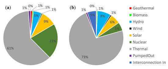
Figure 5.
(a) Electricity generated in Kyushu in 2018 and (b) electricity generated in Japan in 2018.
The hourly sum of the supplies should always equal the demand as described in Equation (1). This condition must be true for each hour and is checked in Step 1 of the methodology:
Demand = Supply
Demand = Geothermal + Biomass + Hydro + Wind + Solar + Nuclear + Thermal ± Pumped storage ± Grid interconnection − SolarPV Curtail − Wind Curtail
To forecast the curtailment, each component of Equation (2) must be calculated for each hour. To facilitate forecasting, these power generation types is categorised based on their observed behaviour. Table 3 depicts the result of classification of power generation types into “controllable” and “non-controllable” with other characteristics such as seasonality, trend, and variability.
Table 3.
Classification of supply and demand types.
Figure 6 depicts the ramp rates, as defined in Equation (3) [24], of the supplies and demand from 05:00 to 19:00 on 7 April 2019, showing how each type reacted to increasing solar power, thus reinforcing the controllable and non-controllable classification.
where P(t) is the VRE power at the target hour and D is the time duration for which the ramp rate is determined (in this case, 1 h intervals based on the input data).
Ramp rate = (P(t) − P(t − D))/D
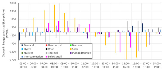
Figure 6.
Ramp rate for each supply type on the highest curtailment day, 7 April 2019, 05:00–19:00.
The main cause of curtailment on this day was solar power, which increased dramatically in the morning, reaching a peak ramp-up rate between 08:00–09:00. Then, it continued to increase at a lower ramp rate up to 12:00, when it started to ramp down. As solar ramped up, the other supply types had to be adjusted to maintain the supply/demand balance, which was what happened initially. However, some types, such as geothermal, biomass, hydro, wind, and nuclear, were not adjusted as the solar ramped up, and they remained mostly constant. These supplies are classified as “non-controllable”, as mentioned earlier, because Kyuden has little to no influence over these supplies. This includes solar, as they cannot control its ramp rate. Demand is also classified as “non-controllable”.
As time progressed, thermal continues ramping down, but it was limited to a maximum ramp down rate of −578 MW/h. The thermal supply presumably approached its minimum generation value at 09:00, and therefore, its ramp rate decreased and eventually approached 0. As this happened, the ramp-up rate of both pumped storage and grid interconnection increased. Grid interconnection, like pumped storage, had a positive and a negative value when it sent more energy to the neighbouring Chugoku region, which was ramping up. However, the large ramp-up of solar power was unable to be matched by the adjustments of the controllable supplies, and therefore, curtailment started ramping up at 07:00, reaching a peak of 685 MW/h between 08:00 and 09:00, as thermal started ramping down.
As the solar ramp-up rate decreased, curtailment continued as peak solar generation occurred at 12:00, and the ramp rate of pumped storage went negative, indicating that the charging rate was reduced, perhaps due to the maximum capacity being reached. Then, the solar ramp rate went negative, indicating that solar was ramping down. In the late afternoon, the ramp-down rate of solar curtailment was reduced to zero; therefore, curtailment stopped at 16:00, at which point thermal started to ramp up, and the balance was maintained as the solar ramp rate was also reduced. Pumped storage had a high ramp down rate between 16:00 and 18:00, as its charging rate decreased to almost zero.
These classifications can be applied to the main supply/demand formula, as defined in Equations (4)–(6):
Demand = (Non-controllable supplies) + (Controllable supplies)
(Non-controllable supplies) = Geothermal + Biomass + Hydro + Wind + Solar + Nuclear
(Controllable supplies) = Thermal ± Pumped storage ± Grid interconnection − SolarPV Curtail − Wind Curtail
2.2. Method
2.2.1. Logic Method: Forecasting Controllable Supplies
The novelty of this research is to develop a model that can forecast curtailment by firstly separating the hourly supply/demand data into two categories namely “non-controllable” and “controllable” and then subtracting the non-controllable supplies from the demand leaving the total controllable supplies but without the distribution of these controllable supplies. Then using a logic method, created for this research, to distribute this total controllable supply among the four types of controllable supplies namely thermal, pumped storage, grid interconnection and curtailment. This method takes the operational limits of each type (hourly max/min and max ramp/min ramp), the priority of curtailment mitigation [9] and the forecasted future installed capacity trends into account with each supply type overflowing to the next type, until all the total controllable supplies have been distributed.
The concept of this novel method comes from observing the raw data and identifying their patterns in step 2. The logic method is named after the logical tests being performed. The main input of the logic model is the hourly non-controllable supplies, the monthly trend for the controllable supplies and the hourly max/min values and hourly max ramp/min ramp (referred to as the max/min table) values for each controllable type (The source code of the logic method is available from the Supplementary Material).
The max/min table contains the limitations for max, min, max ramp and min ramp for each controllable type from the hour 00:00 to 24:00. This results in 4 × 24 = 96 values and 4 values for each hour for each controllable type. This is the key to the operation of the logic model, as it determines the operational windows that each controllable supply can operate in.
The method essentially determines whether each hourly non-controllable value can be assigned to thermal by checking whether the value violates the windows set by the max/min table, as shown in Figure 7. If the window is not violated, then the entire non-controllable value can be assigned to thermal. However, if one of the windows is violated, then it modifies the value until it fits within the operating window, and then the modification value is carried over to the next controllable supply. Then, this is repeated for pumped storage and grid interconnection, and any modified value after grid interconnection is allocated to curtailment.
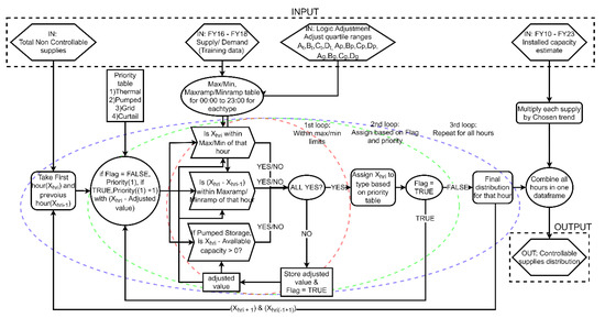
Figure 7.
Logic method flowchart.
The logical checks of the method are as follows based on the values of X(hr(i)), the value of the total non-controllable supplies of a specific hour (i), and of X(hr(i−1)), the value of the total non-controllable supplies for the previous hour (i − 1).
- Is the value of X(hr(i)) within the limits set by the max/min table for that hour?
- Is the value of (X(hr(i)) − X(hr(i−1))) within the ramp limits set by the max/min table for that hour?
- If working on pumped storage and pumped storage is required to supply energy, is there still available capacity left in the system?
Figure 8 exhibits the comparison of the cumulative solar curtailment between the observed (red line) and the predicted (blue line) without calibration for one year from October 2018 to September 2019. The blue line indicates the predicted value without calibration using the default hourly max/min and hourly max ramp/min ramp values far from the actual cumulative curtailment in red. The label at the top left of the Figure 8 using the suffix “A” and four numbers refer to the modification of the max/min table; “A” means all, i.e., all the controllable supply types (thermal, pumped storage and grid interconnection); and the numbers show the modification of those supply types. Thus, in this case, all supply types were left to default values of 1, 0, 1, and 0. In the following calibration process, these will be modified.
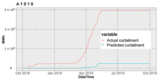
Figure 8.
Comparison between uncalibrated cumulative curtailment forecast (blue line) and actual cumulative curtailment (red line) from October 2018 to September 2019.
2.2.2. Calibration
The calibration is to change the max/min table parameters, effectively adjusting the max, min, max ramp and min ramp windows smaller and then rerunning the logic model so that the forecasted controllable supplies are more in tune with the observed actual value. This is done by iteration through all the possibilities that exist with the 4 parameters, as shown in Figure 9. This ends up as 2n−1, with n being the number of parameters (24 − 1 = 15). Therefore, there are 15 different combinations of the four window parameters that influence each individual controllable type.
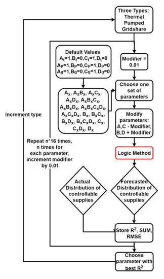
Figure 9.
Calibration method flowchart. A, B, C, and D indicate the calibration parameters with subscript t representing thermal, p for pumped storage, and g for grid interconnection. The default values for four parameters are 1, 0, 1, and 0. Then, they are being adjusted by the modifier with 0.01 value during calibration.
Each of these parameters is then modified by a modifier, which is 0.01 or 1% in this case. The modifier changes the max/min table. For example, the default value of A is 1. This represents 100%, as in the true max value, and then the modifier reduces the size of the max window by 1% (0.01) at each iteration.
Once all 16 parameters have been cycled through, then the modifier increases by 1%, and the cycle is repeated until a set number of cycles (n) are achieved, typically 20. The modifier starts at 1% and ends at 20% in increments of 1% resulting in 320 individual parameter adjustments. Since these parameters adjust the max and min values, the smallest adjustment would be preferable. The 20% was deemed as a maximum limit of adjustment due to its proximity to 3rd (75%) and 1st (25%) quartile respectively.
Ideally, it would be best to cycle through all these combinations for 12 parameters, Ax, AxBx, …, CxDx, and Dx, in Figure 9. However, due to a long calibration time, the calibration is only run on one supply type at a time. Then, the time required for calibration is reduced dramatically and become very practical for real-time operation. After each iteration, the calibration result is compared to observed non-controllable supplies in terms of several statistical measures. Then, the calibrated results are used for the next forecasting.
The statistical indices used are the R², Sum%, RMSE, Sum Pos and Sum Neg (Table 4). The output of the calibration technique is shown in Table 5, with the calibration parameters indicating the four window parameters, the hourly max/min values and hourly max ramp/min ramp values, used for all the controllable types. Note that due the inherent inability to accurately forecast hourly data due to the many externalities, R² was not used in determining which calibration method to choose. The focus was on the general goodness of fit, determined by the other parameters and observation.
Table 4.
Statistical indices description and formula.
Table 5.
Four window calibration parameters used and calibration results for supplies and curtailment as shown in Figure 8.
2.3. Mitigation Measures
After the calibration and validation, scenario-based mitigation measures to the long-term forecasted curtailment were applied and evaluated by measuring their mitigation performance and cost effectiveness. Table 6 shows the mitigation scenarios used for curtailment measures by considering the monthly trends of demand and supplies by generation types.
Table 6.
Explanation of mitigation scenarios considered in this study.
3. Results
3.1. Calibration and Validation: Individual Best Curtailment Sum
Calibration and validation of the logic method to forecast curtailment can be conducted in several different ways. These are based on which characteristics are considered as criteria. The statistical indices are not always the best indication of fit, so some different options are chosen based on observed fit, highest R² and RMSE and best curtailment sum. In this section, the best result of calibration and validation is presented, and the results of other different paths for calibration are demonstrated in Appendix A.
The best result of calibration and validation is obtained with observation-based criterion. This case focuses more on the goodness of fit and the Sum% in the statistical indices. For the four window parameters, the values of (1, 0.06, 0.94, 0.06) are chosen for thermal (T), as they produce the best results, as shown in Figure 10a. These values are then used to calibrate the pumped storage (P), leading to the best results of (0.93, 0, 1, 0.07) presented in Figure 10b. Compared to that of the other calibration and validation cases in Appendix A, the goodness of fit is not as good until late April, underestimating the curtailment after April. However, the sum% of the curtailment is very high at 98.9%, the best result observed yet, with a low amount of solar neg. Finally, these parameters are used to calibrate the grid interconnection in Figure 10c. No improvement is achieved, so grid interconnection remains at the default parameter values. This set of parameters is the best for the overall forecasting of the curtailment compared to the observed, testdata2, and therefore is chosen as the best result. These parameters are then used for curtailment forecast to evaluate mitigation measures.
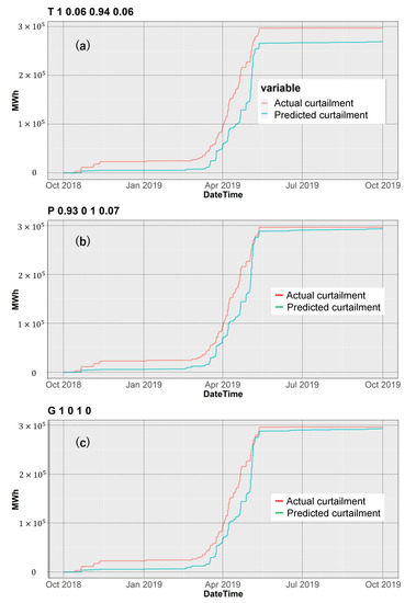
Figure 10.
(a) Validation results with four calibrated parameters of (1, 0.06, 0.94, 0.06) for thermal (T); (b) validation results with four calibrated parameters of (0.93, 0, 1, 0.07) for pumped storage (P); and (c) validation results with four calibrated parameters of (1, 0, 1, 0) for grid interconnection (G). The red lines indicate the actual cumulative curtailments and the blue lines represent the predicted curtailments.
3.2. Mitigation
Figure 11 and Figure 12 show the positive and negative mitigation scenarios, respectively, compared to the forecast curtailment with no mitigation. Table 7 shows those same scenarios in terms of the amount and cost of curtailment as well as the amount and cost of the mitigation scenarios. The second column is the total amount of power (MWp) change that would occur due to the mitigation scenario described. It presents the change in trend and the change in installed capacity calculated by multiplying that change in trend by the 2019 installed capacity [25]. The next column, cost to build, is the average estimated cost to build one MWp of the relevant mitigation technique [3]. These two values are then multiplied together to calculate the total build cost of that mitigation technique.
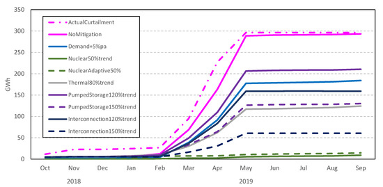
Figure 11.
Cumulative sum of actual curtailment and forecast scenarios that reduced curtailment from October 2018 to September 2019.
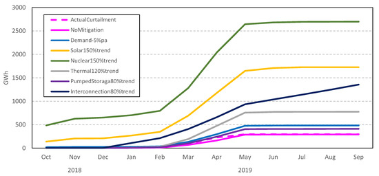
Figure 12.
Cumulative sum of actual curtailment and forecast scenarios that increased curtailment from October 2018 to September 2019.
Table 7.
Effects of mitigation scenarios.
Curtailment in Table 7 is the total curtailment resulting from this mitigation technique, followed by its cost. Then, the calculated curtailment change is presented. This is the change in curtailment from the no mitigation to the relevant mitigation technique. This leads to the curtailment saved column, which indicates how much curtailment was saved due to the implementation of the mitigation techniques. Finally, the balance column shows the difference between the cost to build and the curtailment saved. A positive number indicates that implementing this technique saved money overall, whereas a negative value represents an additional loss in money by implementing this technique.
4. Discussion
Each of the mitigation types is discussed, and the best mitigation measure among the mitigation scenarios considered is presented.
4.1. Demand
Curtailment is very sensitive to any changes in demand, but demand, in this case, is not a mitigation scenario but rather a situation that might occur. The two scenarios used show dramatically different results. If demand were to increase by 5% pa, then there would be ¥3.7 billion less curtailment. However, the more likely scenario is that demand would decrease, which would lead to much higher curtailment, ¥6.5 billion more curtailment than the no mitigation curtailment. Currently, the demand is very stable, but as the ageing population problem worsens, this decreasing demand scenario may be realized, giving extra incentive to implement some of the mitigation techniques.
4.2. Solar
Solar curtailment is directly related to solar generation. Therefore, it is expected that changes in the solar trend would drastically affect curtailment, and this is what is observed. The installed capacity costs were sourced from [26]. Another scenario that could occur is an increasing trend of solar radiation. This would, as expected, lead to high curtailment, significantly higher at ¥48.8 billion. Increasing this solar trend would also require additional solar to be built, estimated at 5505 MWp over the next 4 years, costing ¥1271.2 billion. There would also be many positives to this increased solar production, and perhaps one of the best curtailment mitigation techniques could be applied with this increased solar to mitigate the higher curtailment.
4.3. Nuclear
Next, is nuclear, which exerts substantial control over curtailment. Of the three scenarios presented, two reduced curtailment and one increased curtailment. The two that reduced curtailment were the options that reduced nuclear, namely, nuclear reduced by 50% and adaptive nuclear. Of these techniques, adaptive nuclear appears to be the most realistic, as the 50% reduction in nuclear requires additional nuclear plants to be shut down, which has a large, undeterminable cost. The adaptive scenario aims to line up the curtailment seasons and maintenance schedules. Applying this scenario reduces curtailment by ¥9.5 billion over one year, while having no real associated costs. It is unknown whether this is a realistic scenario and whether the selected 50% shutdown was too much. However, this simulation shows that this type of scenario would reduce curtailment proportionately to the amount of nuclear power that could be adaptively shut down. The scenario in which curtailment increased was when the nuclear trend increased. This is because nuclear has a large influence over VRE curtailment. In this example, increasing the nuclear trend by 50% increased curtailment by ¥81.7 billion and cost ¥631.7 billion. The costs used for the nuclear-installed capacity are referred to in [27].
4.4. Thermal
Thermal also has a significant impact on curtailment but not in a way that might be expected. Increasing thermal actually increases curtailment, whereas decreasing thermal decreases curtailment. This behaviour is due to the simple fact that when thermal is increased, the minimum amount of thermal that can be produced increases, as this newly added thermal also has a minimum operating capacity, which is added to the total thermal minimum operating capacity. However, changing the composition of the thermal generation, such as reducing coal and increasing gas, should reduce curtailment, as coal cannot ramp down rapidly, whereas gas can. This was not one of the scenarios because of the lack of hourly information about coal, oil and gas thermal generation, as discussed in step 2.
Returning to the thermal scenarios, reducing thermal by 80% reduced curtailment by ¥5.7 billion; this scenario does not consider the cost of shutting down 20% of thermal capacity but assumes that some of the existing old thermal capacity may be reaching the end of its usable lifetime. This shows that there is an incentive to shut it down, not only for the reduction in CO2 but also for curtailment reduction. Increasing thermal energy has a significant cost in installed capacity of ¥414.3 billion and an extra ¥16.4 billion in curtailment generated. Therefore, this scenario should be avoided at all costs. The data for the thermal installed capacity cost is referred to in [28].
4.5. Pumped Storage
Pumped storage, as mentioned, is a great accompanying supply with VRE, as it can help shift the peak generation to a later time in the day when VRE generation is lower. Therefore, increasing this supply decreases curtailment, whereas decreasing this supply increases curtailment. This relationship was expected. However, the cost vs. benefit was not as good as expected. The reason for this is that pumped storage is very expensive and requires a long time to build. Furthermore, it is very geographically selective, as it has some specific site requirements for construction. Therefore, increasing pumped storage capacity, especially to reduce curtailment, is not the most efficient solution. Other energy storage measures, such as large-scale batteries, might help in the same way and in a quicker timeframe but still have a significant cost associated with them and were not considered in this study.
Regarding the results in Table 7, it is interesting to note that increasing pumped storage reduces curtailment. However, increasing it further does not reduce curtailment to the same scale, indicating that a smaller installed capacity of pumped storage might be the most efficient solution if it were not for all the mentioned limitations. Overall, increasing pumped storage led to a negative balance, suggesting that this is not the best mitigation technique. Pumped storage can be used in ways other than just for curtailment mitigation, which might change the benefit. However, that is out of the scope of this research. The data for the installed capacity cost came from [29].
4.6. Grid Interconnection
Lastly, the curtailment mitigation scenarios involve grid interconnection trend adjustments. Increasing grid interconnection would decrease curtailment and vice versa, as expected, similar to pumped storage. However, unlike pumped storage, improving the grid interconnection between regions has many additional benefits as its shifts from a fragmented nationwide grid network to a more unified grid network where the overall flexibility increases, greatly improving the overall resilience to curtailment. One crucial point is that, for example, if Kyushu and Chugoku were both facing curtailment issues, they could separately try to fix the problem by changing the installed capacity of some types, as shown above, costing each of them a large amount of money and either reducing overall efficiency (if using storage), thereby losing money from shutting down nuclear energy and requiring more thermal energy in off-peak periods leading to higher CO2 emissions, or simply increasing thermal directly leading to the same problems. Kyushu and Chugoku could improve the grid interconnection between themselves and the Kansai Region, for example, which has high demand and high thermal generation and, therefore, has a high tolerance to curtailment. By doing so, they would be sharing their curtailment tolerance and thereby increase the overall amount of VRE that could be installed with minimal curtailment. This would have to be done together with the OCCTO to ensure that all grid codes and guideline were met but would allow for greater renewable energy penetration, furthermore, this strategy could be applied across Japan for even grid flexibility and therefore higher CP ratio.
There are also several other benefits of a fully connected electricity grid, such as resilience to disasters and an increased ability to handle unexpected events. Therefore, in an examination of the results of the grid interconnection scenario, it is important to understand the additional benefits that come with it. Based only on Kyushu’s curtailment, the balance comes to -¥149.1 billion. The data for the grid interconnection installed capacity cost come from [30,31].
5. Conclusions
The objectives of this study were to understand the underlying causes of curtailment in Kyushu, calculate curtailment and then apply mitigation techniques to reduce curtailment. Curtailment has several influencing factors. However, the main factors that were identified were the highly variable solar generation in low demand times and high constant nuclear generation. Coupled with low inter-grid transfer capability between regions, this means that when an imbalance between supply and demand occurs, there is no choice but to curtail. These problems highlight the need for curtailment forecasting, but due to the recent nature of curtailment in Japan, little research has been conducted. Therefore, a new forecasting method was developed. This method operates under the idea that each controllable type (thermal, pumped storage and grid interconnection) tries to adjust to ensure the supply-demand balance. However, they each have upper and lower limitations in both energy generation and ramp rate that vary within a 24-h period. The logic method tries to allocate the total non-controllable amount to thermal on an hour-by-hour basis. If the amount to be allocated exceeds the operating limits set by the max/min operating windows, then the difference is calculated and passed to pumped storage. This process repeats for pumped storage and then grid share. If there is any remaining energy that cannot be allocated, this is then classified as curtailment.
This method initially returned inaccurate results. However, after several rounds of calibration, which adjusted the quartile values of the max/min operating windows, the overall accuracy was increased to 97% of the real curtailment. The success of this method in forecasting hourly controllable supplies demonstrates the validity of using such a logic-based method for this type of forecasting. Once the forecasted curtailment was accurate, several mitigation scenarios were applied. However, the time-consuming calibration process for optimizing the parameters can be further investigated and improved by applying artificial intelligence in future works.
The uniqueness of the logic method comes from hourly-based forecasting. Other examples of curtailment forecasting use monthly or yearly data, but since the curtailment is very sensitive to the supply-demand balance, any small changes hour by hour could affect curtailment. Therefore, the logic method is unique in its forecasting process and potentially more accurate, as there is no averaging occurring.
The best technique in terms of mitigating curtailment is to make the solar generation trend constant. However, this is not in line with Japan’s 2030 energy goals, nor is it the most environmentally friendly idea. Decreasing thermal or nuclear trends have the second and third best cost-to-benefit ratios. However, decreasing the generation of one type would prevent the other from working, and decreasing nuclear generation would go against Kyuden’s plans of restoring nuclear to post-2011 levels. In the longer term, Kyuden is planning to build additional nuclear reactors, further reducing the likelihood of this idea. Adaptive nuclear shutdown, however, seems to be a good compromise if it is technically and economically possible. The last techniques of increasing either pumped storage or grid interconnection are not economically viable if their only purpose is to reduce curtailment. However, the many other benefits they offer might help to offset their costs.
Ultimately, the decision to implement any of these mitigation techniques comes down to Kyuden. With the current regulations in place, Kyuden has little incentive to reduce curtailment, as IPP-generated VRE is in direct competition with its own generation for which it paid. Unless the government steps in or the regulations change, curtailment will continue until a point where it is above the 8% without compensation limit. After that, Kyuden will be actively losing money when it curtails, which would then provide an incentive to implement mitigation measures/techniques. The problem lies with the fact that none of these mitigation techniques can be implemented quickly. They require foresight of the future problem and investment now, while the problem is still relatively small. Currently, Kyuden and the Japanese government seem unaware and unconcerned with this problem, as if they do not fully understand the future magnitude of the problem. The final goal of this research is to raise awareness and show the future magnitude of the curtailment and its costs and make several mitigation technique recommendations that Kyuden and policymakers may use to prevent the future waste of energy and help improve the ever-growing problem of global warming.
Supplementary Materials
The following are available online at https://www.mdpi.com/1996-1073/13/18/4703/s1, the source code of logic method using R with the observed, testdata2, data used in this study is available as supplementary material.
Author Contributions
Conceptualization, A.B. and H.S.L.; methodology, A.B.; validation, A.B., and H.S.L.; formal analysis, A.B.; investigation, A.B. and H.S.L.; data curation, A.B. and H.S.L.; writing—original draft preparation, A.B.; writing—review and editing, H.S.L.; visualization, A.B.; supervision, H.S.L.; funding acquisition, H.S.L. All authors have read and agreed to the published version of the manuscript.
Funding
This research received no external funding.
Acknowledgments
The hourly supply and demand data were obtained from Kyuden, the electricity company in Kyushu. The first author is supported by the JICE ABE Initiative Program. This research is partly supported by the Grant-in-Aid for Scientific Research (17K06577) from JSPS, Japan.
Conflicts of Interest
The authors declare no conflict of interest.
Abbreviations
| VRE | variable renewable energy |
| PV | photovoltaic |
| FIT | feed-in tariff |
| SPF | scheduled power flow |
| TTC | total transfer capability |
| CP | Curtailment and penetration |
| IPP | independent power producers |
| ISEP | Institute for Sustainable Energy Policies |
| MWh | Megawatt Hour |
| MWp | Megawatt Peak |
| RMSE | Root mean square error |
| OCCTO | Organization for Cross-regional Coordination of Transmission |
Appendix A. Calibration of the Logic Method
As described in the main body text, there are several different ways that the calibration method can be run. These are based on which characteristics are the most important. The statistical indices are not always the best indication of fit, so some different options are chosen based on observed fit, highest R2 and RSME and best curtailment sum. In the following, the results of these different paths for calibration are demonstrated in detail. In some cases, the best results are chosen with one type, and then the next type is calculated, whereas in some cases, the same parameters are applied to all types.
Appendix A.1. Case 1: Individual, Highest R2 and Lowest RMSE
The first case chosen is the highest R² and RMSE for each type. After the calibration is run for thermal, the results are sorted by the highest R² and lowest RMSE, which gives the parameters of (0.88, 0, 1, 0.12) in Figure A1a. The result is better than that of no calibration. However, it shows some strange behaviour by forecasting some curtailment during the period when nuclear was shut down after May. Since it is the first type, no conclusions can be made. These thermal parameters are then used in the pumped storage calibration, and once again, the results resorted by R² and RMSE, which gives the parameters of (1, 0.1, 0.9, 0.1). Figure A1b displays more amplified behaviour of cumulative curtailment in the blue line, and the solar sum negative is −3427 MWh, indicating a significant problem. However, there is one more type to calibrate. Grid interconnection is then calibrated using the previously calculated thermal and pumped storage parameters, and here, the best solar curtailment sum% is chosen. The overall behaviour of Figure A1c is far from testdata2, with significant curtailment forecasted in the period after the May nuclear shutdown; while the overall curtailment sum% is good, there is still quite significant negative curtailment. In the end, this method does not produce good results.
Appendix A.2. Case 2: All Types, Best-Observed Fit
Instead of individually calibrating each controllable type, the other method is to calibrate all types with the same parameters and choose the best results based on the best fit of solar curtailment and observation. The results from this approach are quite improved, as shown in Figure A2, with (1, 0.04, 1,0) applied to each type, resulting in a 94.5% curtailment sum and good behaviour in terms of shutting down when the nuclear stops in mid-May. The sum negative amount is also quite low, at only −110 MWh, which is within the margin for error. Overall, this approach is much better than the R² and RMSE methods. However, there may be better results if each type is calibrated individually and the parameters are chosen by observed fit, which will be performed next.

Figure A1.
(a) Calibration result T0.88,0,1,0.12; (b) calibration result P1,0.1,0.9,0.1; and (c) calibration result G0.9,0.1,0.9,0.1. The red lines indicate the actual cumulative curtailments and the blue lines represent the predicted curtailments.
Figure A1.
(a) Calibration result T0.88,0,1,0.12; (b) calibration result P1,0.1,0.9,0.1; and (c) calibration result G0.9,0.1,0.9,0.1. The red lines indicate the actual cumulative curtailments and the blue lines represent the predicted curtailments.


Figure A2.
Calibration result—A1, 0.04, 1, 0. The red line indicates the actual cumulative curtailments and the blue line represents the predicted curtailments.
Figure A2.
Calibration result—A1, 0.04, 1, 0. The red line indicates the actual cumulative curtailments and the blue line represents the predicted curtailments.

Appendix A.3. Case 3: Individual, Best-Observed Fit
In this case, the results are chosen specifically for their goodness of fit. The values of (1, 0.06, 0.94, 0.06) are chosen for thermal, as these parameters result in a good fit, as shown in Figure A3a. Next, the values of (1, 0.03, 1, 0) are chosen for pumped storage, as shown in Figure A3b. Here, the fit is very good for the entire period until late April, when there is a significant overestimation. Last, these parameters are applied to the grid interconnection in Figure A3c. However, the result do not show any better results than those of the original values, and therefore, the parameters chosen for grid interconnection are the default parameters. Based on this final result in Figure A3c, the overestimation cannot be ignored. Therefore, even though it has the best fit, it is rejected as the best method.


Figure A3.
(a) Calibration result—T1,0.06,0.94,0.06; (b) calibration result—P1,0.03,1,0; and (c) calibration result—G1,0,1,0. The red lines indicate the actual cumulative curtailments and the blue lines represent the predicted curtailments.
Figure A3.
(a) Calibration result—T1,0.06,0.94,0.06; (b) calibration result—P1,0.03,1,0; and (c) calibration result—G1,0,1,0. The red lines indicate the actual cumulative curtailments and the blue lines represent the predicted curtailments.


References
- Japan’s Kyushu Elec Restricts Renewable Energy Supplies for First Time. Available online: https://www.reuters.com/article/japan-nuclear-renewables-restrictions/japans-kyushu-elec-restricts-renewable-energy-supplies-for-first-time-idUSL4N1WS390 (accessed on 10 November 2018).
- Kimura, K. Feed-In Tariffs in Japan: Five Years of Achievements and Future Challenges; Renewable Energy Institute: Tokyo, Japan, 2017; pp. 1–22. [Google Scholar]
- METI. Agency for Natural Resources and Energy. In Ministry of Economy. Japan’s Energy-20 Questions to Understand the Current Energy Situation; Ministry of Economy, Trade and Industry: Tokyo, Japan, 2018. [Google Scholar]
- Bird, L.; Cochran, J.; Wang, X. Wind and Solar Energy Curtailment: Experience and Practices in the United States; National Renewable Energy Laboratory: Denver, CO, USA, 2014. [Google Scholar]
- Kyushu Electric Restricts Renewable Energy Supplies for First Time. Available online: https://japantoday.com/category/business/Kyushu-Electric-restricts-renewable-energy-supplies-for-first-time (accessed on 10 November 2018).
- Institute for Sustainible Energy Policy. Status of Renewable Energies in Japan. 2017. Available online: http://www.isep.or.jp/en/wp/wp-content/uploads/2017/08/ISEP20170827JapanStatus-EN.pdf (accessed on 12 January 2018).
- Mesmer, M. (Email Correspondance). Private communication, 2019.
- Kimura, K. Solar Power Generation Costs in Japan: Current Status and Future Outlook; Renewable Energy Institute: Tokyo, Japan, 2019. [Google Scholar]
- Kyuden Electric Company. Kyuden Annual Report 2019; Kyuden Group: Kyushu, Japan, 2019; Available online: https://www.kyuden.co.jp/var/rev0/0251/9954/f24tslnz.pdf (accessed on 6 October 2019).
- Yasuda, Y.; Bird, L.; Carlini, E.M.; Estanqueiro, A.; Flynn, D.; Forcione, A.; Lázaro, E.G.; Higgins, P.; Holttinen, H.; Lew, D.; et al. International Comparison of Wind and Solar Curtailment Ratio. In WIW2015 Workshop Brussels; Wind Integration Workshop: Brussels, Belgium, 2015; pp. 1–6. [Google Scholar]
- Kokichi, D. Interview, Hiroshima City. 2018.
- OCCTO. Outlook of Electricity Supply–Demand and Cross-regional Interconnection Lines: Actual Data for FY2018. 2018. Available online: https://www.occto.or.jp/en/information_disclosure/outlook_of_electricity_supply-demand/190909_outlook_of_electricity.html (accessed on 1 September 2019).
- OCCTO. OCCTO Annual Report. 2016. Available online: https://www.occto.or.jp/en/information_disclosure/annual_report/files/annual_report_FY2016.pdf (accessed on 3 September 2019).
- Bird, L.; Lew, D.; Milligan, M.; Carlini, E.M.; Estanqueiro, A.; Flynn, D.; Gomez-Lazaro, E.; Holttinen, H.; Menemenlis, N.; Orths, A.; et al. Wind and solar energy curtailment: A review of international experience. Renew. Sustain. Energy Rev. 2016, 65, 577–586. [Google Scholar] [CrossRef]
- Eurostat. Total Gross Electricity Generation. 2014. Available online: http://ec.europa.eu/eurostat/tgm/table.do?tab=table&init=1&language=en&pcode=ten00087&plugin=1 (accessed on 17 April 2015).
- Bundesnetzagentur. Monitoringreport. 2013. Available online: http://www.bundesnetzagentur.de/SharedDocs/Downloads/EN/BNetzA/PressSection/ReportsPublications/2013/MonitoringReport2013.pdf (accessed on 10 July 2019).
- California ISO. Managing Oversupply. 2020. Available online: http://www.caiso.com/informed/Pages/ManagingOversupply.aspx (accessed on 15 March 2020).
- Golden, R.; Paulos, B. Curtailment of Renewable Energy in California and Beyond. Electr. J. 2015, 28, 36–50. [Google Scholar] [CrossRef]
- Suganthi, L.; Samuel, A.A. Energy models for demand forecasting—A review. Renew. Sustain. Energy Rev. 2012, 16, 1223–1240. [Google Scholar] [CrossRef]
- Hyndman, R.J.; Athanasopoulos, G. Forecasting: Principles and Practice, 2nd ed.; OTexts: Melbourne, Australia, 2018. [Google Scholar]
- Yanagisawa, A. Population Decline and Electricity Demand in Japan: Myth and Facts; The Institute of Energy Economics, Japan: Tokyo, Japan, 2015. [Google Scholar]
- Kyuden Electric Company. System Information Disclosure. 2020. Available online: http://www.kyuden.co.jp/wheeling_disclosure.html (accessed on 1 February 2020).
- Institute for Sustainible Energy Policy. ISEP Supply Demand. 2020. Available online: https://isep-energychart.com/en/graphics/electricityproduction/?region=all&period_year=2016&period_month=4&period_day=1&period_length=1+week&display_format=residual_demand (accessed on 15 March 2020).
- Japanese Government. ESTAT. 2018. Available online: https://www.e-stat.go.jp/en/regional-statistics/ssdsview/prefectures (accessed on 30 December 2019).
- Abuella, M.; Chowdhury, B. Forecasting of solar power ramp events: A post-processing approach. Renew. Energy 2019, 133, 1380–1392. [Google Scholar] [CrossRef]
- IRENA. Renewable Power Generation Costs in 2017; International Renewable Energy Agency: Abu Dhabi, UAE, 2018. [Google Scholar]
- Matsuo, Y.; Nei, M. Assessing the Historical Trend of Nuclear Power Plant Construction Costs in Japan; The Institute of Energy Economics, Japan: Tokyo, Japan, 2018. [Google Scholar]
- EIA. Cost and Performance Characteristics of New Generating Technologies. Annu. Energy Outlook 2019 2019, 2019, 1–3. [Google Scholar]
- Manwaring, M.; Rodgers, K.; Flake, S.; Erpenbeck, D. Pumped Storage Report; National Hydropower Association: Washington, DC, USA, 2018. [Google Scholar]
- Cory, B. Pricing in electricity transmission and distribution. Proc. Mediterr. Electrotech. Conf.-MELECON 2014, 1, 19–25. [Google Scholar]
- OCCTO. Studying the Planning Process for the Interconnection Between Kyushu and Chugoku; OCCTO: Tokyo, Japan, 2018. [Google Scholar]


© 2020 by the authors. Licensee MDPI, Basel, Switzerland. This article is an open access article distributed under the terms and conditions of the Creative Commons Attribution (CC BY) license (http://creativecommons.org/licenses/by/4.0/).