An Integrally Embedded Discrete Fracture Model for Flow Simulation in Anisotropic Formations

Abstract

The embedded discrete fracture model (EDFM), among different flow simulation models, achieves a good balance between efficiency and accuracy. In the EDFM, micro-scale fractures that cannot be characterized individually need to be homogenized into the matrix, which may bring anisotropy into the matrix. However, the simplified matrix–fracture fluid exchange assumption makes it difficult for EDFM to address the anisotropic flow. In this paper, an integrally embedded discrete fracture model (iEDFM) suitable for anisotropic formations is proposed. Structured mesh is employed for the anisotropic matrix, and the fracture element, which consists of a group of connected fractures, is integrally embedded in the matrix grid. An analytic pressure distribution is derived for the point source in anisotropic formation expressed by permeability tensor, and applied to the matrix–fracture transmissibility calculation. Two case studies were conducted and compared with the analytic solution or fine grid result to demonstrate the advantage and applicability of iEDFM to address anisotropic formation. In addition, a two-phase flow example with a reported dataset was studied to analyze the effect of the matrix anisotropy on the simulation result, which also showed the feasibility of iEDFM to address anisotropic formation with complex fracture networks.

1. Introduction

With the increasing demand for energy, the development of reservoirs bearing essential resources, such as oil and gas, is of great importance. In many exploitation practices, the target reservoirs are naturally fractured [1,2]. During the development of the reservoirs, numerical simulation is a reasonable and affordable tool to manage production and evaluate economic feasibility. A number of numerical models for fractured reservoir have been established in the past several decades.

The dual porosity model (DPM), with the assumption of fracture and matrix uniformity, was proposed as one of the earliest methods [3,4,5]. In addition to the subsequent multi-continuum methods, such as dual-porosity dual-permeability (DPDK) model [6,7], multiple interacting continua (MINC) model [8,9], subdomain model [10], triple porosity dual-permeability (TPDK) model [11,12] and multi-porosity model [13], the DPM provides an efficient approach to simulate micro-scale fractures. However, it is also limited by the loss of detailed information relating to discovered macro-scale factures, such as geometry and location [14].

The discrete fracture model (DFM) uses unstructured grids to discretize the discovered macro-scale fractures explicitly, which is more physics-based and accurate [15,16,17,18,19,20], but is limited because of its complexity in gridding and computational cost [19]. Therefore, improvements of the DFM have mainly been focused on calculation efficiency. For example, by applying the fracture crossflow equilibrium (FCFE) approach to DFM, the grid orientation is lowered, and the flux calculation is more accurate than the traditional finite element (FE) and control volume finite element (CVFE) methods in the DFM [21,22,23].

The embedded discrete fracture model (EDFM) [19,24,25,26,27,28,29] is another alternative. As a compromise, it uses Cartesian gridding for the matrix, as in DPM, to reduce the calculation cost, but also discretizes macro-scale fractures explicitly, as in DFM, to account for the complexity of the fractures. However, in the EDFM, a uniform pressure gradient is assumed in the matrix grid and a fracture is usually required to be discretized into many segments [30,31]. Some improved EDFMs have been proposed to solve this problem. For example, projection-based Embedded Discrete Fracture Model (pEDFM) [32,33] automatically scales the matrix–matrix connections in the vicinity of fracture networks. An integrally embedded discrete fracture model (iEDFM) [30] was also proposed to improve simulation accuracy and expand the applications to fractures with complex geometry.

The simplified matrix–fracture fluid exchange assumption also makes it difficult for these EDFM approaches to address the anisotropic flow between the fracture and matrix. Most naturally fractured reservoirs contain multiple-length scaled fractures. In the aforementioned DFM and EDFM, the discovered macro-scale fractures are discretized explicitly, but micro-scale fractures are often difficult to characterize individually, so have to be homogenized into a matrix continuum. Due to the complex geological conditions, the development of these micro-scale fractures could show an advantageous orientation, making the effective matrix continuum anisotropic [34]. In addition, the advantageous orientation during the deposition of rock particles could be another cause of matrix anisotropy [35].

In this paper, an integrally embedded discrete fracture model (iEDFM) suitable for anisotropic formations is proposed. In this model, a structured mesh is employed for the anisotropic matrix system, and a fracture element, which consists of several fracture segments or a group of connected fractures, is integrally embedded in the matrix grid. For the plane radial flow problem, continuous coordinate rotation is often used to map the solution of anisotropic formation to that of equivalent isotropic formations [35,36,37,38], which is very effective when dealing with anisotropic flow inside the matrix continuum. Based on the radial flow theory, a semi-analytic matrix–fracture transmissibility calculation method specially designed for anisotropic formation is presented for the iEDFM.

This paper is organized as follows. Firstly, the methodology is introduced, including the basic mathematical method, the derivation of the steady flow pressure distribution formula of a point source in an anisotropic formation expressed by permeability tensor, and the algorithm for the embedding of fractures into the anisotropic formation. Subsequently, the applicability of the proposed iEDFM for anisotropic formation is demonstrated by comparison with an analytic solution. We also demonstrate the advantage of iEDFM by comparing its results with those of a fine grid and of an EDFM ignoring the anisotropy during matrix–fracture transmissibility calculation. Finally, the effect of the matrix anisotropy on two-phase flow in a fractured reservoir is analyzed through a modified case with a reported dataset, which also shows the feasibility of the proposed iEDFM to address anisotropic formation with complex fracture networks.

2. Methodology

2.1. Basic Mathematical Method

A multidimensional black-oil method for an anisotropic isothermal system is adopted in this paper. The mass-balance equation is given by:

$$\frac{\partial }{\partial t}\left(\phi S_{\beta }{\rho }_{\beta }\right)=-\nabla ·\left({\rho }_{\beta }{{\displaystyle v}}_{\beta }\right)+q_{\beta }$$

(1)

where $\beta$ represents different components: $\beta =g$ stands for gas, $\beta =w$ stands for water, and $\beta =o$ stands for oil; $\phi$ is the effective porosity; $S_{\beta }$ is the saturation of $\beta$; ${\rho }_{\beta }$ is the density of $\beta$; $q_{\beta }$ is the sink/source term; and ${{\displaystyle v}}_{\beta }$ is the velocity of $\beta$, which can be defined by Darcy’s law:

$$v_{\beta }=-\frac{k_{r\hspace{0.17em}\beta }}{{\mu }_{\beta }}K·\left(\nabla P_{\beta }-{\rho }_{\beta }g\nabla D\right)$$

(2)

$$K=\left(\begin{array}{ccc}{k}_{xx}& k_{xy}& k_{xz}\\ k_{xy}& k_{yy}& k_{yz}\\ k_{xz}& k_{yx}& k_{zz}\end{array}\right)$$

(3)

where $K$ is an absolute permeability tensor; $k_{r\hspace{0.17em}\beta }$ is the relative permeability to $\beta$; ${\mu }_{\beta }$ is the viscosity of $\beta$; $P_{\beta }$ is the pressure of $\beta$ under reservoir conditions; $g$ is gravitational acceleration; $D$ is the depth from the reference datum.

For a certain porous medium, the permeability and the velocity under a certain pressure gradient are determined, but the component of the permeability tensor and velocity vector varies with different coordinate systems. If the coordinate axis is rotated to an appropriate direction where $k_{xy}=k_{yz}=k_{xz}=0$, the coordinate axis direction becomes the principal axis direction of the permeability. The permeability tensor is diagonal as follows:

$$K=\left(\begin{array}{ccc}{k}_{XX}& 0& 0\\ 0& k_{YY}& 0\\ 0& 0& k_{ZZ}\end{array}\right)$$

(4)

For example, tensor diagonalization for two-dimensional cases can be obtained as:

$$k_{XX}=\frac{1}{2}\left[k_{xx}+k_{yy}+\sqrt{{\left(k_{xx}-k_{yy}\right)}^2+4k_{xy}^2}\right]$$

(5)

$$k_{YY}=\frac{1}{2}\left[k_{xx}+k_{yy}-\sqrt{{\left(k_{xx}-k_{yy}\right)}^2+4k_{xy}^2}\right]$$

(6)

Unless otherwise stated, the coordinate axis direction in this paper is considered rotated to the principal axis direction of the permeability, where $k_{xy}=k_{yz}=k_{xz}=0$. Therefore, we can use $k_x$, $k_y$, $k_z$ to represent the absolute permeability in three directions. In addition, the embedding algorithm when the two sets of axes do not coincide is also introduced, which can be applied in simulators that support permeability tensor.

As implemented numerically, Equation (1) is written into discretized form with an integral finite-difference or control-volume scheme in the space domain, and a finite-difference, backward, first-order scheme in the time domain [11]:

$$\left\{{\left(\phi S_{\beta }\hspace{0.17em}{\rho }_{\beta }\right)}_i^{n+1}-{\left(\phi S_{\beta }{\rho }_{\beta }\right)}_i^n\right\}\frac{V_i}{\Delta t}={\displaystyle \sum _{j\in {\eta }_i}{F}_{\beta ,ij}^{n+1}}+Q_{\beta ,i}^{n+1}$$

(7)

where $n$ is the previous time level; $n+1$ is the current time level; $\Delta t$ is the time step size; $V_i$ is the volume of element $i$; ${\eta }_i$ contains the set of neighboring elements $j$ to which element $i$ is directly connected; $Q_{\beta ,i}^{}$ is the sink/source term at element $i$; $F_{\beta ,ij}^{}$ is the flow term between element $i$ and $j$, which can be described by a discrete version of Darcy’s law, given by:

$$F_{\beta ,ij}^{}={\lambda }_{\beta ,ij+1/2}{T}_{i\hspace{0.17em}j}\left[\left(P_{\beta ,j}^{}-{\rho }_{\beta ,ij+1/2}^{}\hspace{0.17em}\hspace{0.17em}g{D}_j\right)-\left(P_{\beta ,i}^{}-{\rho }_{\beta ,ij+1/2}^{}\hspace{0.17em}\hspace{0.17em}g{D}_i\right)\right]$$

(8)

where $D_i$ is the depth from the reference datum to the center of element $i$; $ij+1/2$ is a proper averaging or weighting of properties; ${\lambda }_{\beta ,ij+1/2}$ is the mobility term, defined as:

$${\lambda }_{\beta ,ij+1/2}^{}={\left(\frac{{\rho }_{\beta }{k}_{r\beta }}{{\mu }_{\beta }}\right)}_{ij+1/2}$$

(9)

where $T_{ij}$ is transmissibility, which is the harmonic average of $T_i$ (element $i$ to common interface) and $T_j$ (element $j$ to common interface):

$$T_{ij}=\frac{T_i\cdot T_j}{T_i+T_j}$$

(10)

$$T_i=\frac{A_{ij}\hspace{0.17em}{k}_i}{d_i}, T_j=\frac{A_{ij}\hspace{0.17em}{k}_j}{d_j}$$

(11)

where $A_{ij}$ is the common interface area between elements $i$ and $j$; $d_i$ and $d_j$ are the feature distances; $k_i$ and $k_j$ are the absolute permeability along each element center to the interface. The specific physical meaning of the parameters varies for different connections, which will be discussed in the next section.

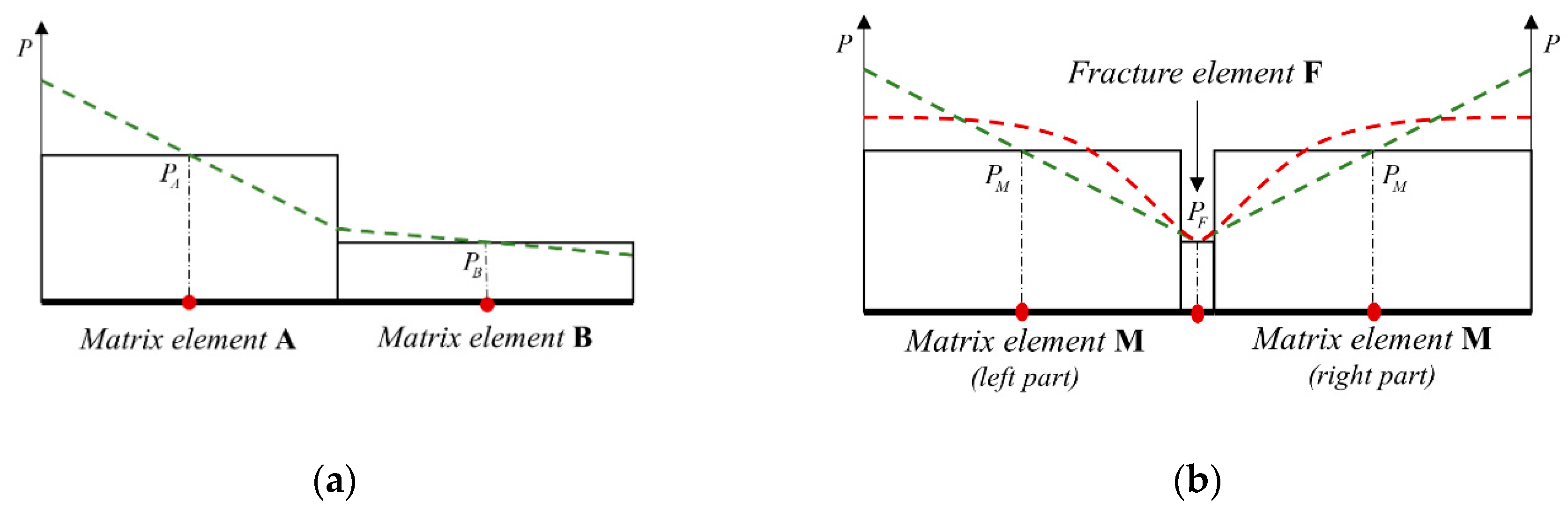
2.2. Integrally Embedded Discrete Fracture Model

The integrally embedded discrete fracture model (iEDFM) is a pre-processor with the inputs of reservoir features and fracture geometries, and outputs of element and connection information. It is implemented on EDFM with a different gridding method. In this work, a new transmissibility calculation method for matrix–fracture connection in iEDFM suitable for anisotropic formation is presented, based on a more realistic pressure distribution assumption in the vicinity of fractures inside the anisotropic matrix element domain. The transmissibility can be determined before simulation, so it can be easily implemented in various simulators.

In EDFM/iEDFM, Cartesian grids are used for the matrix. Every fracture element consists of one or several connected fractures. Each fracture element is connected with its corresponding matrix element. Thus, there mainly exist 3 kinds of connections: matrix–matrix (M–M), fracture–fracture (F–F), and matrix-fracture (M–F). Due to the existence of wells, well-matrix/fracture is also an important connection. The focus of this work is on the flow between fractures and the matrix, so the vertical wells are simplified as sink points.

In Figure 1, we illustrate the procedure to discretize fracture elements with a 2D case with 4 matrix blocks and 2 intersecting fractures. Six fracture elements will be generated in the EDFM, as shown in Figure 1a. Both the boundary of the matrix blocks and intersection of the two fractures discretize the fracture elements. Meanwhile, in iEDFM, the fractures can be embedded integrally—either discretizing by only matrix block boundaries (Figure 1b) or taking the whole intersecting fracture group as one element (Figure 1c) is permitted. As a result, the number of fracture elements, as well as the number of F–F and F–M connections, can be reduced. In iEDFM(II), the entire set of the intersecting fracture group is regarded as a single element, which is also an equipotential body, thus, the fluid velocity through this fracture group is infinite. It is obviously an ideal approximation, only suitable for a situation where the fracture permeability is far greater than the matrix. Therefore, iEDFM(I) is more recommended for more realistic situations.

The pressure difference between adjacent fracture elements is relatively small due to the high conductivity in the fracture. Therefore, the coarser discretization method of iEDFM can reduce calculation costs and improve the convergence [30].

The transmissibility of the three kinds of connections can be calculated referring to Equations (10) and (11) but with different physical meaning of the parameters:

For M–M connections, the permeability difference between the two connected elements is relatively small, and the pressure inside each element domain nearly has a linear distribution (shown by the green line in Figure 2a), which approximately meets the assumption of one-dimensional Darcy flow. Thus, the parameters give clear physical meanings: the feature distance $d_i$ and $d_j$ are the distances between the center of each matrix element to the common interface; and the absolute permeability $k_i$ and $k_j$ are equal to the matrix permeability $k_x$, $k_y$ or $k_z$ because the Cartesian matrix block is usually built in the direction of the coordinate system.

For F–F connections, the physical meanings of parameters are also clear for the same reason: $d_i$ and $d_j$ are the shortest distances from the center of each fracture element along the fracture direction to the common interface; $k_i$ and $k_j$ are fracture permeability $k_F$.

For M–F connections, $T_F$ is much larger than $T_M$. Thus, according to Equation (10), $T_{M-F}$ is approximately equal to $T_M$. Because there is a large difference between the permeability of the matrix and the fracture, the pressure inside the matrix element domain in the vicinity of the fracture nearly has a cone distribution (as shown by red line in Figure 2b). Thus, if we still assume the pressure has a linear distribution (as shown by the green line in Figure 2b) to use the one-dimensional Darcy flow equation, non-negligible errors may be introduced when calculating $T_{M-F}$. To avoid this, a common idea is to further subdivide the matrix meshes in the vicinity of the fracture to approximate the cone pressure distribution, which is why the DFM needs denser matrix meshes around the fracture.

EDFM chooses not to add extra matrix elements to maintain efficiency, and still follows the assumption of a linear distribution of pressure, which may introduce errors, especially when the matrix mesh is coarsely divided or the fracture needs to be subdivided due to its complex geometry [27,30].

In iEDFM, neither the matrix nor the fracture is required to be subdivided. Furthermore, $T_{M-F}$ is solved based on a more realistic pressure distribution derived by a semi-analytic algorithm for anisotropic formation, which will be discussed in the next section.

2.3. Algorithm for the Embedding of Fractures into Anisotropic Formation

The complexity of fracture geometry and anisotropy of the matrix can strongly influence or even dominate the matrix–fracture fluid exchange. Therefore, calculation methods for $T_{M-F}$ are the key point to embed fractures into the anisotropic formation.

To calculate $T_{M-F}$, an analytic solution of pressure distribution around a point source in an anisotropic formation is introduced. Then, we assume that there are a series of point sources distributed along the fractures. With the flow strength of each point source calculated, the semi-analytic pressure distribution inside the anisotropic matrix domain can be obtained by integrating the analytic solution of all the point sources. Finally, the pressure distribution is used to compute the value of $T_{M-F}$.

In this section, the algorithm for 2D cases (gravity ignored) in which the coordinate axis direction coincides with the principal axis direction of the permeability are both considered.

2.3.1. Analytic Point-Source Solution in Anisotropic Formation

As shown in Figure 3a, when the coordinate axis direction coincides with the principal axis direction of the permeability, $k_{xy}=k_{yx}=0$. The flow strength of the point source can be obtained as (Appendix A presents the detailed derivation):

$$q=\frac{2\pi rh\sqrt{k_x{k}_y}}{\mu }\frac{\partial P}{\partial r}$$

(12)

where $h$ is the thickness of the reservoir.

The steady-state equation of a point source is:

$$k_x\frac{{\partial }^{2}P}{\partial x^2}+k_y\frac{{\partial }^{2}P}{\partial y^2}=0$$

(13)

By introducing an anisotropy coefficient $\beta =\sqrt{k_x/k_y}$, we can transform the problem of anisotropic formation into an equivalent form for isotropic formation as:

$$\frac{{\partial }^{2}P}{\partial X^2}+\frac{{\partial }^{2}P}{\partial Y^2}=0$$

(14)

where:

$$X=\sqrt{{\beta }^{-1}}\cdot x, Y=\sqrt{\beta }\cdot y$$

(15)

The inner boundary condition is:

$$q=\frac{2\pi h\sqrt{k_x{k}_y}}{\mu }{\left[r\frac{\partial P}{\partial r}\right]}_{r\to 0}$$

(16)

Thus, the solution of the steady-state equation can be obtained as:

$$\begin{array}{l}P\left(x,y\right)=\frac{q\mu }{4\pi hk}\ln \left[X^2+Y^2\right]+C\\ =\frac{q\mu }{4\pi h\sqrt{k_x{k}_y}}\ln \left[\sqrt{\frac{k_y}{k_x}}{x}^2+\sqrt{\frac{k_x}{k_y}}{y}^2\right]+C\end{array}$$

(17)

As shown in Figure 3b, when an angle ${\theta }_k\ne 0$ exists between the coordinate axis direction ($xoy$) and the principal axis direction of the permeability ($\zeta o\eta$), $k_{xy}=k_{yx}\ne 0$. By the coordinate transformation procedures (Appendix B presents the detailed derivation), the point-source solution can be obtained as:

$$P\left(x,y\right)=\frac{q\mu }{4\pi h\sqrt{k_{xx}{k}_{yy}-k_{xy}^2}}\ln \left[\frac{k_{yy}{x}^2+k_{xx}{y}^2+2k_{xy}xy}{\sqrt{k_{xx}{k}_{yy}-k_{xy}^2}}\right]+C$$

(18)

2.3.2. Calculation Methods for Matrix–Fracture Transmissibility

We assume there are a series of point sources $S_i\left(x_{S_i},y_{S_i}\right)$ ($i$ = 1 to N, normally N > 50) distributed along the fractures to calculate the pressure distribution inside the anisotropic matrix domain.

Based on the superposition principle of potential, the pressure of any point $X\left(x,y\right)$ inside the matrix domain can be obtained from the integral of Equations (17) or (18):

$$P_X\left(x,y\right)={\displaystyle \sum _{i=1}^N\frac{q_{S_i}\mu }{2\pi h{k}_e}\ln r_{e,iX}}+C$$

(19)

where $q_{S_i}$ is the flow strength of point-source $S_i$; $k_e$ is the equivalent permeability; and $r_{e,iX}$ is the equivalent distance between this point $X$ to point source $S_i$.

$$k_e=\sqrt{k_{xx}{k}_{yy}-k_{xy}^2}$$

(20)

$$r_{e,iX}=\frac{1}{\sqrt{k_e}}\sqrt{k_{yy}{\left(x-x_{S_i}\right)}^2+k_{xx}{\left(y-y_{S_i}\right)}^2+2k_{xy}\left(x-x_{S_i}\right)\left(y-y_{S_i}\right)}$$

(21)

If the coordinate axis direction coincides with the principal axis direction of the permeability, we have $k_{xy}=k_{yx}=0$ and the Equations (20) and (21) can be written as:

$$k_e=\sqrt{k_x{k}_y}$$

(22)

$$r_{e,iX}=\frac{1}{\sqrt{k_e}}\sqrt{k_y{\left(x-x_{S_i}\right)}^2+k_x{\left(y-y_{S_i}\right)}^2}$$

(23)

As shown in Figure 4b, a series of reference points $F_j$ ($j$ = 1 to N, the same number as for point sources) on the surface of the fracture can be used to determine the unknown parameters $q_{S_i}$ and $C$ in Equation (19).

If these reference points are on the surface of a same fracture element, they could be assumed to have the same pressure $P_F$. Then, Equation (19) can be established for every reference point, forming an N-dimensional linear equation system:

$$P_F={\displaystyle \sum _{i=1}^N\frac{q_{S_i}\mu }{2\pi h{k}_e}\ln r_{e,ij}}+C (j=1\mathrm{to} \mathrm{N})$$

(24)

where $r_{e,ij}$ is the equivalent distance between the point source S_i and the reference point $F_j$.

If we define:

$${\xi }_i=\frac{q_{S_i}}{P_F-C}$$

(25)

where ${\xi }_i$ can be solved out from the linear system Equation (24), then, the pressure of any point $X$ $\left(x,y\right)$ inside the matrix domain can be written as:

$$P_X\left(x,y\right)={\displaystyle \sum _{i=1}^N\frac{{\xi }_i\mu \ln r_{e,iX}}{2\pi h{k}_e}}\left(P_F-C\right)+C$$

(26)

In addition, we have:

$$P_M=\frac{1}{V_M}{\displaystyle \underset{M}{\iint }{P}_X\cdot d{V}_X}$$

(27)

where $V_M$ is the volume of this matrix element; $d{V}_x$ is an element volume at point X.

Combining Equations (26) and (27) and the definition equation of transmissibility (Equation (8)), the M–F transmissibility and the pressure anywhere inside the matrix domain can be calculated by:

$$T_{M-F}^{}=\frac{k_e}{\epsilon -1}{\displaystyle \sum _{S_i\in M}{\xi }_i}$$

(28)

$$P_X=\left(\frac{\mu }{2\pi h{k}_e}{\displaystyle \sum _{i=1}^N{\xi }_i\ln r_{e,iX}}-1\right)\cdot \frac{P_M-P_F}{\epsilon -1}+P_F$$

(29)

where $\in M$ means that the point is inside this matrix domain and:

$$\epsilon =\frac{1}{V_M}{\displaystyle \underset{M}{\iint }\frac{1}{2\pi r_{e,iX}}{\displaystyle \sum _{i=1}^N{\xi }_i}d{V}_X}$$

(30)

From Equations (28)–(30), we note that $T_{M-F}$ is only related to the properties of the reservoir and can be determined at the step of pre-processing before the numerical simulation starts.

Regardless of whether the coordinate axis direction coincides with the principal axis direction of the permeability, $T_{M-F}$ can be calculated with $k_e$ and $r_{e,iX}$ in Equations (22) and (23) or Equations (20) and (21).

3. Model Validation

3.1. Case 1: Single-Phase Flow in Anisotropic Formation with Vertical Fractured Well

In a rectangular anisotropic formation of single-phase fluid, the analytic solution of a vertical fractured well at a fixed production rate under a quasi-steady state can be derived.

In this paper, numerical results of a vertical fractured well case are presented and compared with the analytic solution. Various fracture azimuths, anisotropy coefficients, and fracture permeabilities are considered to illustrate the accuracy of iEDFM.

3.1.1. Analytic Solution of Quasi-Steady-State Flow

As shown in Figure 5, the dimensions of the quasi-three-dimensional rectangular reservoir are $x_e\times y_e\times h$, the half-length of the vertical fracture is $x_f^{}$, and the aperture is $w_f$. A vertical well with constant production $q$ is located at the midpoint of the fracture (called a vertical fracture well). The coordinate axis direction coincides with the principal axis direction of the permeability, and the fracture azimuth is $\theta$.

If the formation is isotropic, the analytic solution of the entire reservoir pressure field can be expressed as [35,39,40]:

$$p_{avg}\left(t\right)-p_{wf}=\frac{q\mu }{kh}\left[G_L\left(g_{wr};g_w\right)+f\left(c_{fD}\right)\right]$$

(31)

where $p_{avg}\left(t\right)$ represents the average pressure of the entire rectangular reservoir at time $t$; $p_{wf}$ represents the pressure of the vertical well.

In Equation (31), $G_L\left(g_{wr};g_w\right)$ is a two-point function to characterize the effect of the geometric features, such as the size of the calculation area and the distribution of fractures; the first variable $g_{wr}$ represents the coordinates of the pressure measurement point; the second variable $g_w$ represents the coordinates of the vertical fracture midpoint, that is also the vertical well position. Gringarten [41] proved that the pressure drop at 0.732 half-length of a fracture is equal to the pressure drop of the entire fracture, so the point $\left(x_w+0.732x_f\cos \theta ,y_w+0.732x_f\sin \theta \right)$ is taken as the pressure measurement point.

$f\left(c_{fD}\right)$ is a function to characterize the effect of the fracture permeability. The modified coefficient $c_{fD}$ reflects the influence of relative fracture permeability. The greater the fracture permeability relative to the matrix, the larger the value of $c_{fD}$.

The detailed calculations for the parameters in Equation (31) are given in Appendix C.

To compare the analytic solution with the numerical results of iEDFM, a dimensionless production index $J_D$ is defined as [35]:

$$J_D=\frac{q\mu }{kh\left[p_{avg}\left(t\right)-p_{wf}\right]}={\left[G_L\left(g_{wr};g_w\right)+f\left(c_{fD}\right)\right]}^{-1}$$

(32)

Spivey and Lee [37] equate anisotropic formation with isotropic formation by coordinate transformation. Parameter changes caused by this coordinate transformation are shown in

Table 1. Parameter changes from anisotropic formation to equivalent isotropic formation.

Anisotropic Formation	Equivalent Isotropic Formation
Anisotropy coefficient $\beta$	$\beta =\sqrt{k_x/k_y}$
Coordinate $x$, $y$	$x^{\prime }={\beta }^{-1}x$, $y^{\prime }=\beta y$
Matrix permeability $k_x$, $k_y$	$k=\sqrt{k_x{k}_y}$
Fracture azimuth $\theta$	${\theta }^{\prime }=\arctan \left(\beta \tan \theta \right)$
Fracture Half-length $x_f^{}$	$x_f^{\prime }=x_f^{}\sqrt{{\beta }^{-1}{\cos }^2\theta +\beta {\sin }^2\theta }$
Fracture aperture $w_f$	$w_f^{\prime }=w_f\cos \left({\theta }^{″}-{\theta }^{\prime }\right)\sqrt{{\beta }^{-1}{\sin }^2\theta +\beta {\cos }^2\theta }$

.

After coordinate transformation, the dimensionless production index $J_D$ is written as [35]:

$$J_D={\left[G_L\left(\left(x_w^{\prime }+0.732x_f^{\prime }\cos {\theta }^{\prime },y_w^{\prime }+0.732y_f^{\prime }\sin {\theta }^{\prime }\right);\left(x_w^{\prime },y_w^{\prime }\right)\right)+f\left(c_{fD}^{\prime }\right)\right]}^{-1}$$

(33)

3.1.2. Comparison between Numerical and Analytic Solutions

A numerical case of iEDFM is established referring to Figure 5 with water production at a fixed rate in a micro-compressible rectangular reservoir. We calculate the production index at the pseudo-steady state from the numerical result, and compare it with that calculated from Equation (33).

The basic parameters of the numerical example are shown in

Table 2. Parameters for case 1.

Reservoir	Size $x_e\times y_e\times h$ (m): $800\times 800\times 25$
Matrix	Meshes: $20\times 20\times 1$	Permeability in x direction $k_x$ (m2): ${10}^{-12}$
Fracture	Permeability $k_f$: $w_f^2/12$	Half-length $x_f^{}$ (m): $60\sqrt{2}$ for $\theta =\pi /4$; $60\sqrt{3}$ for $\theta =\pi /3$
Vertical Well	Production $q$ (m3/s): $0.01$	Position $\left(x_w,y_w\right)$: $\left(400,400\right)$

. The remaining parameters can be calculated from different anisotropy coefficients, fracture azimuths, and modified coefficients (fracture permeability) used in this case.

Figure 6 shows the production index $J_D$ when the fracture azimuth $\theta =\pi /4$. Different anisotropy coefficients $\beta$ and modified coefficient $c_{fD}$ are considered. Numerical solutions of nine sets of parameters are presented and compared with the analytic solution.

Figure 7 shows the production index $J_D$ when the fracture azimuth $\theta =\pi /3$. Numerical solutions of 10 sets of parameters are presented and compared.

Figure 8 shows the pseudo-steady-state pressure distribution with fracture azimuth $\theta =\pi /3$ and modified coefficient $c_{fD}=500$. Cases under different anisotropy coefficients are presented. In Figure 8, the injection times are 5 × 10⁵ s (Figure 8a) and 1 × 10⁶ s (Figure 8b); both times represent a pseudo-steady state.

As shown in Figure 6 and Figure 7, the production index $J_D$ increases with $c_{fD}$, namely, the fracture permeability. When the fracture permeability increases to a certain extent, $J_D$ remains flat.

When the fracture azimuth $\theta =\pi /4$, the numerical solutions of $\beta =1/4$ and $\beta =4$ coincide, and the numerical solutions of $\beta =1/2$ and $\beta =2$ also coincide. It can be seen that the entire reservoir has symmetry at this time, and the numerical solution simulates this symmetry.

When fracture azimuth $\theta =\pi /3$, the numerical solution of the production index $J_D$ with $\beta =4$ is greater than that with $\beta =1/4$, and the numerical solution with $\beta =2$ is greater than that with $\beta =1/2$. Because the fracture is biased towards the dominant principal direction of matrix permeability (that is, the y-direction when $\beta >1$), the flow in that direction would be further strengthened and the production would decrease.

In this numerical case, the iEDFM simulation results agree well with the analytic solution in the anisotropic rectangular formation for a single-phase quasi-steady-state problem with a fixed-rate production vertical fracture well, which demonstrates the reliability of iEDFM.

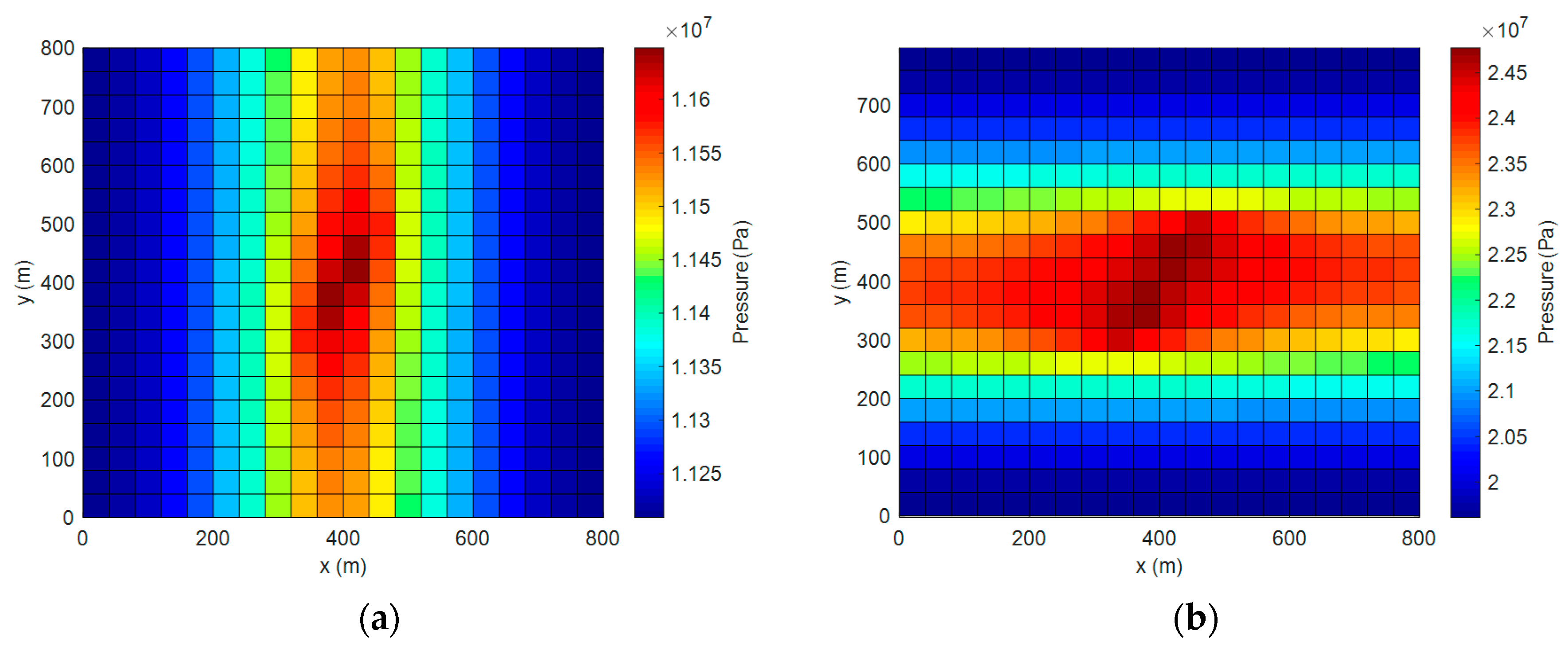
3.2. Case 2: Two-Phase Flow in Anisotropic Formation with Two Crossed Fractures

For the iEDFM of anisotropic formations, matrix–fracture transmissibility is the key issue, as illustrated in Section 2.3.2. In order to investigate the effects of anisotropy on matrix–fracture transmissibility, a water flooding case with a set of intersecting fractures was simulated. In this case, matrix permeability in the y-direction was set to be three times the permeability in the x-direction ($\beta =\sqrt{3}/3$). A fixed rate water injection well (as the blue arrow shows) and a fixed pressure producing well (as the red arrow shows) are implied in this case. The sketch and meshes for iEDFM are shown in Figure 9. The parameters for case 2 are shown in

Table 3. Parameters for case 2.

Reservoir	Size $x\times y$ (m): $1.0\times 1.0$
Matrix	iEDFM mesh: $27\times 27$ Fine grid mesh: $540\times 540$	Permeability $k_x$(m2): $1.0\times {10}^{-14}$ $k_y$(m2): $3.0\times {10}^{-14}$
Fracture	Permeability $k_f$: $1.0\times {10}^{-10}$
Injection Well	Injection $q$ (m3/d): $0.1$	Position: $\left(1.0,0.5\right)$
Producing Well	Pressure $p$ (MPa): $1.0$	Position: $\left(0.0,0.5\right)$

.

In order to further demonstrate the reliability of the iEDFM for anisotropic problems, a comparison with the fine grid result was carried out. In fine grid simulation, the matrix mesh was set as $540\times 540$ and fractures were considered as discretized elements with higher permeability. The same parameters and well settings were used in both iEDFM and fine grid simulations. As shown in Figure 10, the oil production result of iEDFM agrees well with the fine grid result, which shows the reliability and accuracy of the iEDFM for anisotropic formations. In addition, the calculation time of iEDFM was about 12 s, which demonstrates its advantage of calculation efficiency compared with the 133 min required for the fine grid simulation.

In order to investigate the effect of anisotropy on M–F transmissibility, case 2 was simulated under two different circumstances. The anisotropy was considered when calculating the flow between M–M connections under both circumstances, while cases with and without consideration of anisotropy when calculating M–F transmissibility were compared.

The oil saturation distributions at $1\times {10}^7$ s are compared in Figure 11a,b. At this moment, since the displacement front has just reached the two fractures, the oil saturation in the matrix after the displacement front is similar in both cases, but the flow in the fractures appears to be more prominent when anisotropy is not considered in the M–F transmissibility.

The oil saturation distributions at $5\times {10}^7$ s are shown in Figure 11c,d. At this moment, the profiles of oil saturation are rather different between both cases. Fluid flows faster in fractures, which causes the oil saturation around the ends of the fractures to be smaller when M–F transmissibility is calculated without the consideration of anisotropy. The displacement front also progresses further when anisotropy is not considered. These results indicate that if anisotropy is not considered in the calculation of M–F transmissibility, fluid exchange between the matrix and the fracture will be exaggerated, which leads to erroneous simulation results.

Figure 12 shows the comparison of oil rate and oil production between cases with and without consideration of anisotropy when calculating M–F transmissibility. Both oil rate and oil production appear to be smaller with anisotropy is considered, also demonstrating that ignoring the anisotropy when calculating M–F transmissibility will exaggerate fluid exchange between the matrix and the fracture.

Compared with the fine grid result, case 2 further demonstrates the reliability of iEDFM in two-phase flow in anisotropic formations, and also presents the obvious effect of anisotropy on matrix–fracture transmissibility.

4. Model Application

As shown in Figure 13, a quasi-three-dimensional reservoir is considered. The fracture distribution and fracture permeability are adapted from geological survey data of a real reservoir [41,42]. The reservoir thickness is 100 m; the reservoir boundary is enclosed; the equivalent permeability of the matrix $k=\sqrt{k_x{k}_y}$ is 10⁻¹⁴ m²; the fracture permeability is 10⁻⁷ m²; the initial oil saturation is 0.8; the injection well is located at the center of the reservoir and injects water at a constant rate of 4 × 10⁴ m³/day; and four production wells are located at the corners of the reservoir producing at initial pressure.

The matrix of the reservoir is gridded as 25 × 25 × 1 blocks. The fracture network is discretized to 107 fracture elements, of which nine are intersected fracture elements and 22 are non-planer fracture elements.

After 7000 days of injection, the oil rate curve of production well-1, well-2, well-3, well-4 are shown in Figure 14a–d. The oil saturation distribution under various conditions of injection is shown in Figure 15. The average oil saturation of the entire reservoir at 2000 days is 0.5971 ($\beta =1/4$), 0.5655 ($\beta =1$), and 0.5544 ($\beta =4$).

It can be seen from Figure 14 that under different anisotropy coefficients, the breakthrough times of the production wells differ. Although the equivalent permeability remains the same, the oil production efficiency and final oil distribution are different, indicating that the anisotropy of the reservoir greatly affects the fluid flow.

The matrix is homogeneous, the injection well is located at the midpoint, and the production wells are symmetrically distributed. Therefore, if we ignore the fracture network, the oil distribution under $\beta =1/4$ and $\beta =4$ should have a symmetrical relationship. However, it can be seen from Figure 11 that when the fracture network is considered, the oil distribution under $\beta =1/4$ and $\beta =4$ is clearly different. In addition, as the average remaining oil saturation shows, the recovery ratio under $\beta =4$ is much lower than that of the isotropic case and the recovery ratio under $\beta =1/4$ is slightly higher than that of the isotropic case.

These differences demonstrate that the existence of the fracture network can increase the influence of matrix anisotropy. Specifically, the injection water easily breaks into the fracture network, then tends to flow in the direction of higher permeability. If there are production wells in this direction, it is easy to form a breakthrough channel (such as the water channel along the top of Figure 15c). This improves the initial oil recovery, but makes it more difficult to recover the remaining oil. In contrast, if the direction from the fracture end to the nearest production well is not in the direction of lower permeability (such as the situation in Figure 15b), the initial oil recovery is decreased but the total recovery will increase. This characteristic could be significant in the wellsite selection procedure during development of an anisotropic reservoir.

This example shows the applicability of the iEDFM in a more complex situation, and also demonstrates its potential applicability in real field studies.

5. Conclusions

In this paper, an integrally embedded discrete fracture model (iEDFM) suitable for anisotropic formations is proposed. In this model, a structured mesh is employed for the anisotropic matrix system, and a fracture element consisting of several fracture segments or a group of connected fractures is integrally embedded into the matrix grid. A method to calculate the transmissibility between the matrix and the fracture for anisotropic formations is presented.

An anisotropic rectangular reservoir with a fixed-rate production vertical fracture well, a single-phase quasi-steady-state problem, is used to demonstrate the applicability and accuracy of the iEDFM. Different circumstances with various fracture azimuths, anisotropy coefficients, and fracture permeabilities are considered. The simulation results agree well with the analytic solutions. The effect of anisotropy on M–F transmissibility is also investigated. The advantage of the iEDFM is demonstrated by comparison with a fine grid model.

Furthermore, a water flooding example with a modified reported dataset is conducted to analyze the effect of the matrix anisotropy, which also shows the feasibility of the iEDFM to address anisotropic formation with complex fracture networks, and demonstrates potential application of the iEDFM in real field studies.

References

1. Saller, S.P.; Ronayne, M.J.; Long, A.J. Comparison of a Karst Groundwater Model with and without Discrete Conduit Flow. Hydrogeol. J. 2013, 21, 1555–1566. [Google Scholar] [CrossRef]
2. Gurpinar, O.M.; Kossack, C.A. Realistic Numerical Models for Fractured Reservoirs. SPE J. 2000, 5, 485–491. [Google Scholar] [CrossRef]
3. Warren, J.E.; Root, P.J. The Behavior of Naturally Fractured Reservoirs. SPE J. 1963, 33, 245–255. [Google Scholar] [CrossRef] [Green Version]
4. Kazemi, H. Pressure Transient Analysis of Naturally Fractured Reservoirs with Uniform Fracture Distribution. SPE J. 1969, 9, 451–462. [Google Scholar] [CrossRef]
5. Swaan, A.D. Theory of Waterflooding in Fractured Reservoirs. SPE J. 1978, 18, 117–122. [Google Scholar] [CrossRef]
6. Gilman, J.R. Efficient Finite-Difference Method for Simulating Phase Segregation in the Matrix Blocks in Double-Porosity Reservoirs. SPE Reserv. Eng. 1986, 1, 403–413. [Google Scholar] [CrossRef]
7. Gilman, J.R.; Kazemi, H. Improved Calculations for Viscous and Gravity Displacement in Matrix Blocks in Dual-Porosity Simulators. J. Pet. Technol. 1988, 40, 60–70. [Google Scholar] [CrossRef]
8. Pruess, K.; Narasimhan, T.N. Practical Method for Modeling Fluid and Heat Flow in Fractured Porous Media. SPE J. 1985, 25, 14–26. [Google Scholar] [CrossRef] [Green Version]
9. Wu, Y.S.; Pruess, K. Multiple-porosity Method for Simulation of Naturally Fractured Petroleum Reservoirs. SPE Reserv. Eng. 1988, 3, 335–350. [Google Scholar] [CrossRef] [Green Version]
10. Fung, L.S.K. Simulation of Block-to-Block Processes in Naturally Fractured Reservoirs. SPE Reserv. Eng. 1991, 6, 477–484. [Google Scholar] [CrossRef]
11. Wu, Y.; Di, Y.; Kang, Z.; Fakcharoenphol, P. A Multiple-Continuum Model for Simulating Single-phase and Multiphase Flow in Naturally Fractured Vuggy Reservoirs. J. Pet. Sci. Eng. 2011, 78, 13–22. [Google Scholar] [CrossRef]
12. Sun, H.; Chawathe, A.; Hoteit, H.; Shi, X.; Li, L. Understanding Shale Gas Flow Behavior Using Numerical Simulation. SPE J. 2015, 20, 142–154. [Google Scholar] [CrossRef]
13. Yan, B.; Alfi, M.; An, C.; Cao, Y.; Wang, Y.; Killough, J.E. General Multi-porosity Simulation for Fractured Reservoir Modeling. J. Nat. Gas Sci. Eng. 2016, 33, 777–791. [Google Scholar] [CrossRef]
14. Bai, M. On Equivalence of Dual-Porosity Poroelastic Parameters. J. Geophys. Res. Solid Earth 1999, 104, 10461–10466. [Google Scholar] [CrossRef]
15. Noorishad, J.; Mehran, M. An Upstream Finite-Element Method for Solution of Transient Transport-Equation in Fractured Porous-Media. Water Resour. Res. 1982, 18, 588–596. [Google Scholar] [CrossRef] [Green Version]
16. Karimi-Fard, M.; Firoozabadi, A. Numerical Simulation of Water Injection in Fractured Media Using the Discrete-Fracture Model and the Galerkin Method. SPE Reserv. Eval. Eng. 2003, 6, 117–126. [Google Scholar] [CrossRef]
17. Monteagudo, J.; Firoozabadi, A. Control-Volume Method for Numerical Simulation of Two-phase Immiscible Flow in Two- and Three-Dimensional Discrete-Fractured Media. Water Resour. Res. 2004, 40, W07405.1–W07405.20. [Google Scholar] [CrossRef] [Green Version]
18. Hoteit, H.; Firoozabadi, A. Compositional Modeling of Discrete-Fractured Media without Transfer Functions by the Discontinuous Galerkin and Mixed Methods. SPE J. 2006, 11, 341–352. [Google Scholar] [CrossRef]
19. Matthai, S.K.; Mezentsev, A.; Belayneh, M. Finite Element-Node-Centered Finite-Volume Two-Phase-Flow Experiments with Fractured Rock Represented by Unstructured Hybrid-Element Meshes. SPE Reserv. Eval. Eng. 2007, 10, 740–756. [Google Scholar] [CrossRef]
20. Sandve, T.H.; Berre, I.; Nordbotten, J.M. An Efficient Multi-Point Flux Approximation Method for Discrete Fracture-Matrix Simulations. J. Comput. Phys. 2012, 231, 3784–3800. [Google Scholar] [CrossRef]
21. Zidane, A.; Firoozabadi, A. An efficient numerical model for multicomponent compressible flow in fractured porous media. Adv. Water Resour. 2014, 74, 127–147. [Google Scholar] [CrossRef]
22. Zidane, A.; Firoozabadi, A. Fracture-Cross-Flow Equilibrium in Compositional Two-Phase Reservoir Simulation. SPE J. 2017, 22, 950–970. [Google Scholar] [CrossRef]
23. Zidane, A.; Firoozabadi, A. Higher-order simulation of two-phase compositional flow in 3D with non-planar fractures. J. Comput. Phys. 2020, 402, 108896. [Google Scholar] [CrossRef]
24. Li, W.; Dong, Z.; Lei, G. Integrating Embedded Discrete Fracture and Dual-Porosity, Dual-Permeability Methods to Simulate Fluid Flow in Shale Oil Reservoirs. Energies 2017, 10, 1471. [Google Scholar] [CrossRef] [Green Version]
25. Lee, S.H.; Lough, M.F.; Jensen, C.L. Hierarchical Modeling of Flow in Naturally Fractured Formations with Multiple Length Scales. Water Resour. Res. 2001, 37, 443–455. [Google Scholar] [CrossRef]
26. Li, L.; Lee, S.H. Efficient Field-Scale Simulation of Black Oil in a Naturally Fractured Reservoir through Discrete Fracture Networks and Homogenized Media. SPE Reserv. Eval. Eng. 2008, 11, 750–758. [Google Scholar] [CrossRef]
27. Xu, Y.; Cavalcante Filho, J.S.A.; Yu, W.; Sepehrnoori, K. Discrete-Fracture Modeling of Complex Hydraulic-Fracture Geometries in Reservoir Simulators. SPE Reserv. Eval. Eng. 2017, 20, 403–422. [Google Scholar] [CrossRef]
28. Yu, W.; Xu, Y.; Liu, M.; Wu, K.; Sepehrnoori, K. Simulation of Shale Gas Transport and Production with Complex Fractures Using Embedded Discrete Fracture Model. AIChE J. 2018, 64, 2251–2264. [Google Scholar] [CrossRef]
29. Yan, X.; Huang, Z.; Yao, J.; Zhang, Z.; Liu, P.; Li, Y.; Fan, D. Numerical Simulation of Hydro-Mechanical Coupling in Fractured Vuggy Porous Media Using the Equivalent Continuum Model and Embedded Discrete Fracture Model. Adv. Water Resour. 2019, 126, 137–154. [Google Scholar] [CrossRef]
30. Shao, R.; Di, Y. An Integrally Embedded Discrete Fracture Model with a Semi-Analytic Transmissibility Calculation Method. Energies 2018, 11, 3491. [Google Scholar] [CrossRef] [Green Version]
31. Yan, B.; Mi, L.; Chai, Z.; Wang, Y.; Killough, J.E. An Enhanced Discrete Fracture Network Model for Multiphase Flow in Fractured Reservoirs. J. Petrol. Sci. Eng. 2018, 161, 667–682. [Google Scholar] [CrossRef]
32. Rao, X.; Cheng, L.; Cao, R.; Jia, P.; Liu, H.; Du, X. A Modified Projection-Based Embedded Discrete Fracture Model (pEDFM) for Practical and Accurate Numerical Simulation of Fractured Reservoir. J. Petrol. Sci. Eng. 2020, 187, 106852. [Google Scholar] [CrossRef]
33. Tene, M.; Bosma, S.B.M.; Al Kobaisi, M.S.; Hajibeygi, H. Projection-Based Embedded Discrete Fracture Model (pEDFM). Adv. Water Resour. 2017, 105, 205–216. [Google Scholar] [CrossRef]
34. Zeng, Q.; Yao, J.; Shao, J. Study of Hydraulic Fracturing in an Anisotropic Poroelastic Medium via a Hybrid EDFM-XFEM Approach. Comput. Geotech. 2019, 105, 51–68. [Google Scholar] [CrossRef]
35. Xu, W.; Wang, X.; Xing, G.; Wang, J. Pressure-Transient Analysis for a Vertically Fractured Well at an Arbitrary Azimuth in a Rectangular Anisotropic Reservoir. J. Petrol. Sci. Eng. 2017, 159, 279–294. [Google Scholar] [CrossRef]
36. Craig, D.P.; Blasingame, T.A. Constant-Rate Drawdown Solutions Derived for Multiple Arbitrarily-Oriented Uniform-Flux, Infinite-Conductivity, or Finite-Conductivity Fractures in an Infinite-Slab Reservoir. In Proceedings of the SPE Gas Technology Symposium, Calgary, AB, Canada, 15–18 May 2006. [Google Scholar]
37. Spivey, J.P.; Lee, W.J. Estimating the Pressure-Transient Response for a Horizontal or a Hydraulically Fractured Well at an Arbitrary Orientation in an Anisotropic Reservoir. SPE Reserv. Eval. Eng. 1999, 2, 462–469. [Google Scholar] [CrossRef]
38. Kucuk, F.; Brigham, W.E. Transient Flow in Elliptical Systems. SPE J. 1979, 19, 401–410. [Google Scholar] [CrossRef]
39. Wang, L.; Wang, X.; Ding, X.; Zhang, L.; Li, C. Rate Decline Curves Analysis of a Vertical Fractured Well with Fracture Face Damage. J. Energ. Resour. Asme. 2012, 134, 032803.1–032803.9. [Google Scholar]
40. Gringarten, A.C.; Ramey, H.J.; Raghavan, R. Unsteady-State Pressure Distributions Created by a Well with a Single Infinite Conductivity Vertical Fracture. SPE J. 1974, 14, 347–360. [Google Scholar] [CrossRef] [Green Version]
41. Zhang, Y.; Gong, B.; Li, J.; Li, H. Discrete Fracture Modeling of 3D Heterogeneous Enhanced Coalbed Methane Recovery with Prismatic Meshing. Energies 2015, 8, 6153–6176. [Google Scholar] [CrossRef] [Green Version]
42. Shuck, E.L.; Davis, T.L.; Benson, R.D. Multicomponent 3-D Characterization of a Coalbed Methane Reservoir. Geophysics 1996, 61, 315–330. [Google Scholar] [CrossRef]
Figure 1. Gridding methods: (a) typical embedded discrete fracture model (EDFM); (b) integrally embedded discrete fracture model (iEDFM)(I)—fracture discretized by matrix block boundaries; (c) iEDFM(II)—taking the whole intersecting fracture group as one fracture element.
Energies 13 03070 g001
Figure 2. Pressure distribution assumption between two connected elements. (a) matrix–matrix (M–M) connection: linear distribution; (b) matrix–fracture (M–F) connection: linear distribution/cone distribution (tally with the actual situation).
Energies 13 03070 g002
Figure 3. Point-source solution when the coordinate axis direction (a) coincides or (b) does not coincide with the principal axis direction of the permeability.
Energies 13 03070 g003
Figure 4. Illustration showing the calculation of M–F transmissibility in iEDFM: (a) a 2D view of the fractured reservoir; (b) the top view of the dotted frame part.
Energies 13 03070 g004
Figure 5. The rectangular formation for the analytic solution of a vertical fractured well at a fixed production rate under a quasi-steady state.
Energies 13 03070 g005
Figure 6. Dimensionless production index J D when fracture azimuth θ = π / 4 .
Energies 13 03070 g006
Figure 7. Dimensionless production index J D when fracture azimuth θ = π / 3 .
Energies 13 03070 g007
Figure 8. Pseudo-steady-state pressure distribution when the fracture azimuth θ = π / 3 for different anisotropy coefficients (a) β = 1 / 4 and (b) β = 4 .
Energies 13 03070 g008
Figure 9. Sketch and meshes of iEDFM for case 2.
Energies 13 03070 g009
Figure 10. Comparison of oil production between the iEDFM and fine grid.
Energies 13 03070 g010
Figure 11. Oil saturation for case 2: (a) anisotropy not considered when calculating M–F transmissibility, t = 1 × 10 7 s; (b) anisotropy considered when calculating M–F transmissibility, t = 1 × 10 7 s; (c) anisotropy not considered when calculating M–F transmissibility, t = 5 × 10 7 s; (d) anisotropy considered when calculating M–F transmissibility, t = 5 × 10 7 s.
Energies 13 03070 g011
Figure 12. Comparison of (a) oil rate and (b) oil production between cases with and without consideration of anisotropy when matrix–fracture transmissibility is calculated.
Energies 13 03070 g012
Figure 13. Sketch and meshes of example for model application.
Energies 13 03070 g013
Figure 14. Oil production rate of each production well under different anisotropy coefficients.
Energies 13 03070 g014
Figure 15. Profiles of oil saturation after 7300 days of injection with: (a) β = 1 (isotropic formation); (b) β = 1 / 4 ; (c) β = 4 .
Energies 13 03070 g015