Frequency Analysis of Solar PV Power to Enable Optimal Building Load Control †


Abstract
1. Introduction
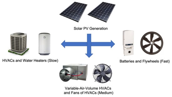
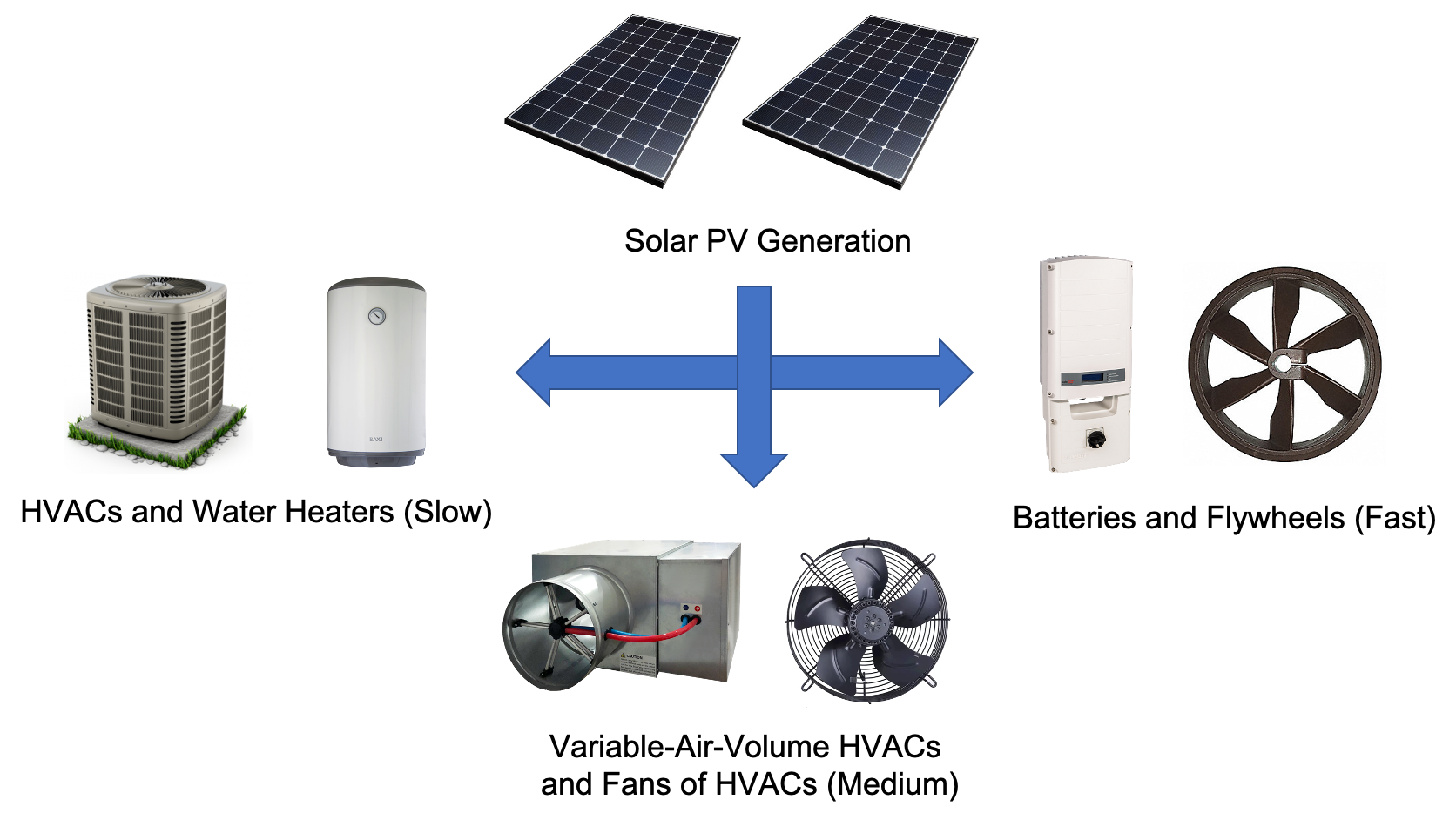
2. Proposed Approach
3. Spectral Analyses of PV Power Generation and Building TCLs Power Consumption
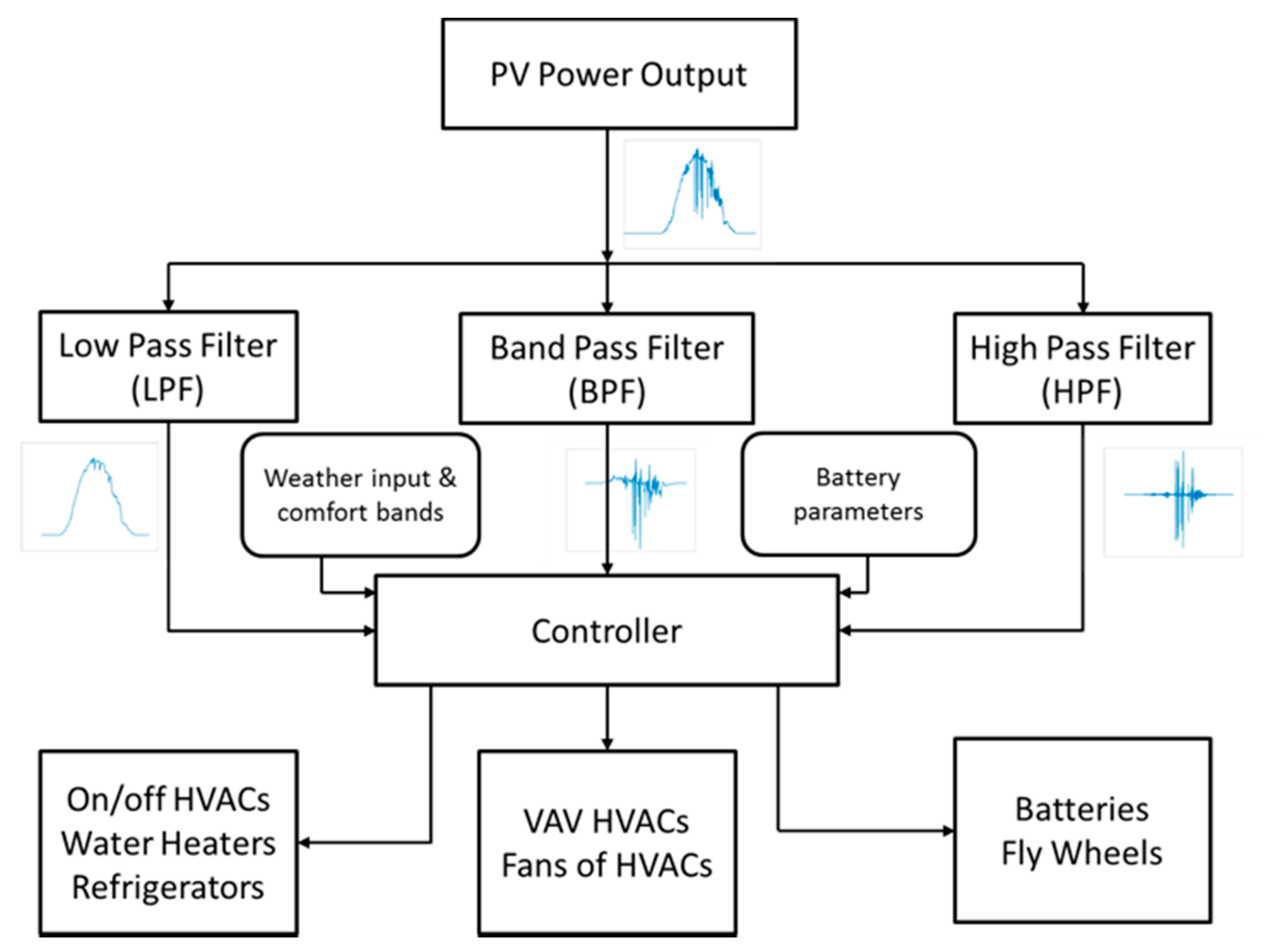
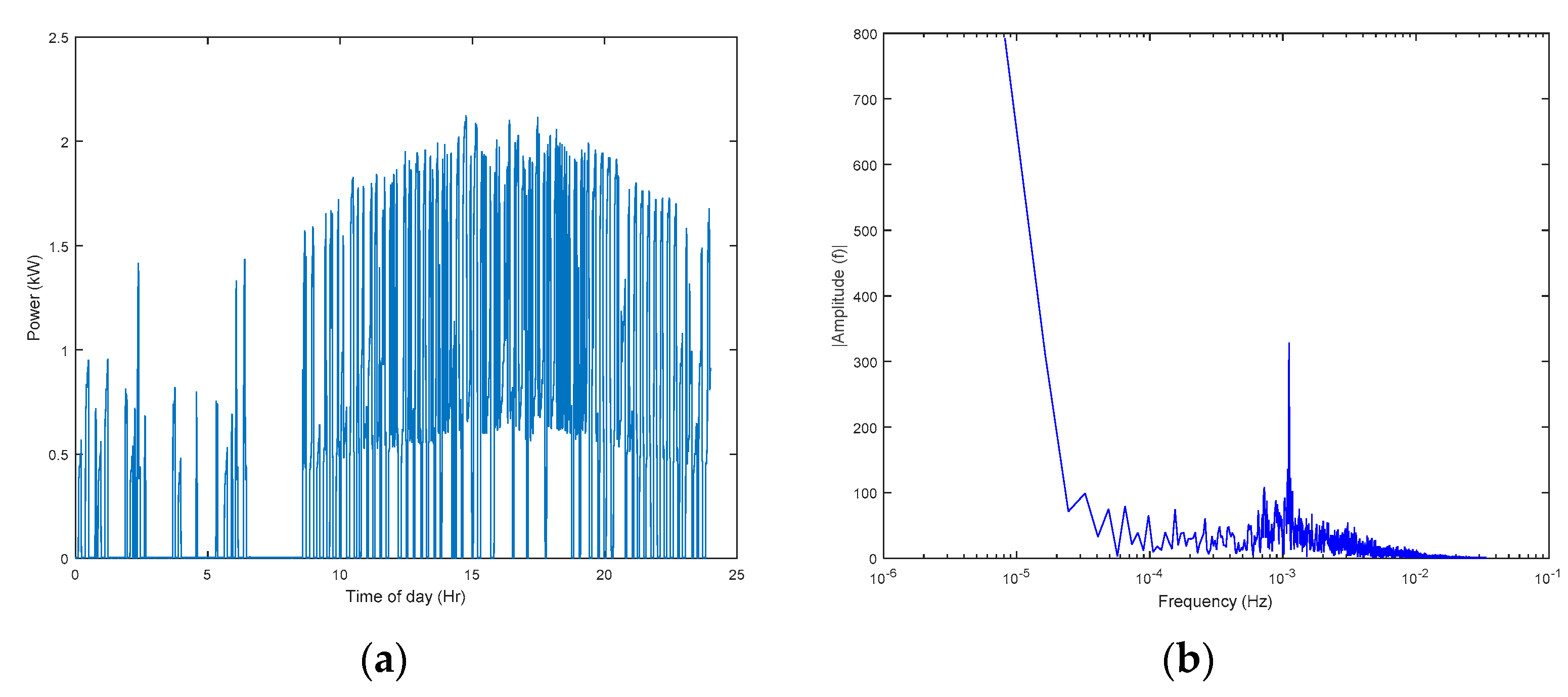
3.1. Solar PV
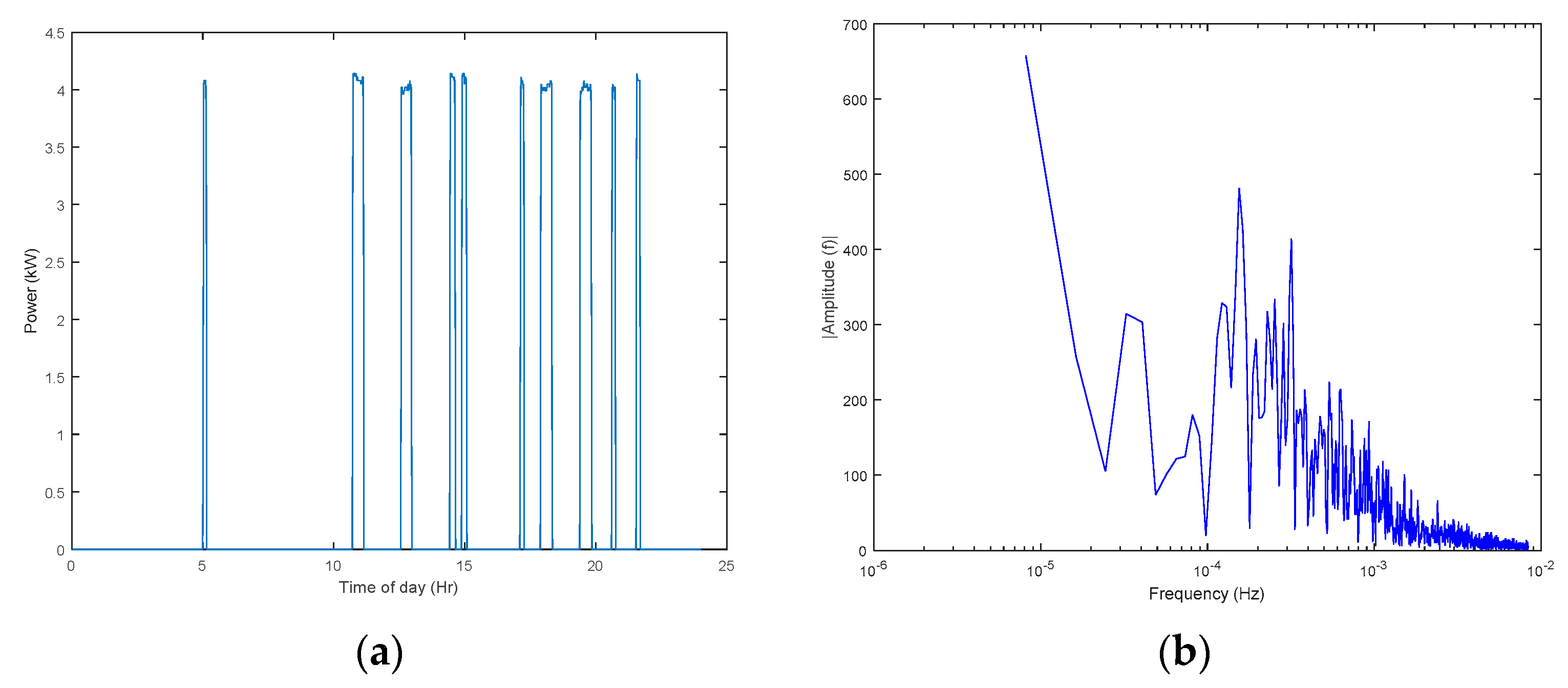
3.2. Building TCLs
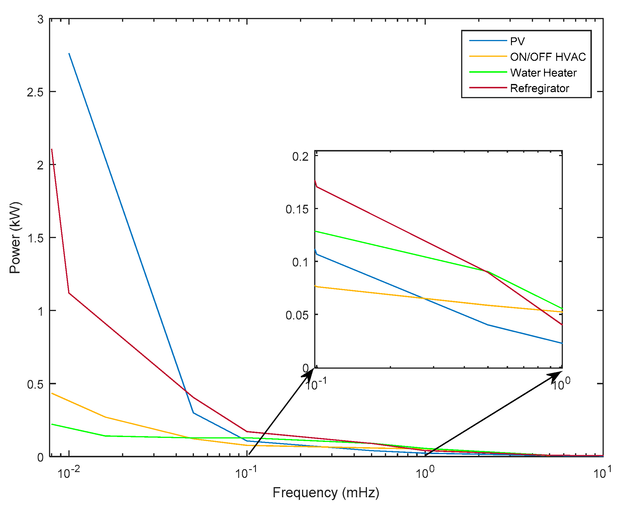
3.3. Comparison
4. Model Predictive Control of Building TCLs
4.1. Building TCLs
4.1.1. HVAC Model
4.1.2. Water Heater
4.1.3. Refrigeration System
4.1.4. Building Model
4.2. MPC Design
5. Case Studies
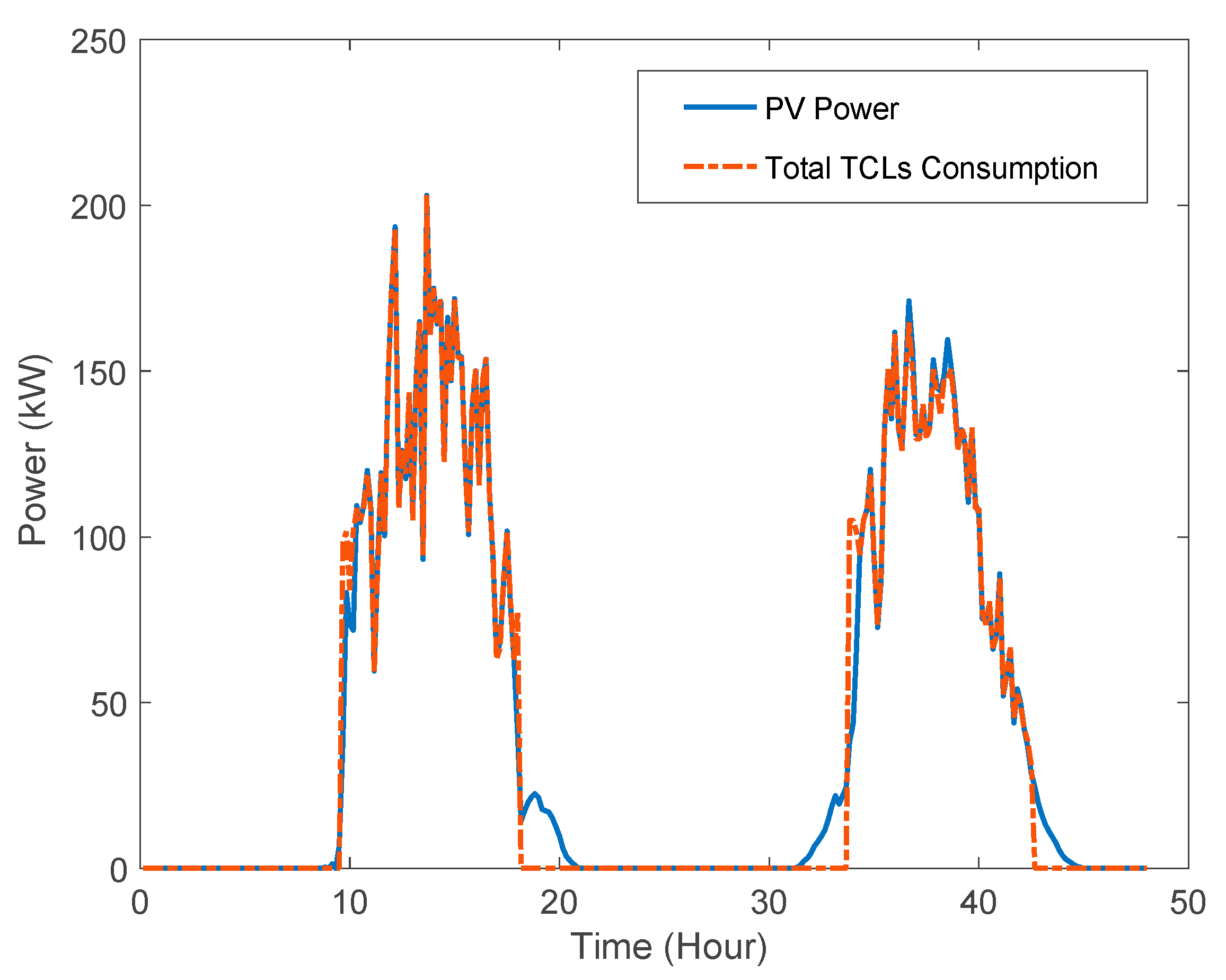
5.1. Low and Medium Frequency Contents of PV Power
5.2. High Frequency Contents of PV Power
6. Conclusions
Author Contributions
Funding
Acknowledgments
Conflicts of Interest
References
- Xu, Z.B.; Guan, X.H.; Jia, Q.S.; Wu, J.; Wang, D.; Chen, S.Y. Performance Analysis and Comparison on Energy Storage Devices for Smart Building Energy Management. IEEE Trans. Smart Grid 2012, 3, 2136–2147. [Google Scholar] [CrossRef]
- Williams, C.; Binder, J.; Kelm, T. Demand side management through heat pumps, thermal storage and battery storage to increase local self-consumption and grid compatibility of PV systems. In Proceedings of the 2012 3rd IEEE PES Innovative Smart Grid Technologies Europe (ISGT Europe), Berlin, Germany, 14–17 October 2012; pp. 1–6. [Google Scholar]
- Zhou, T.; Sun, W. Optimization of Battery–Supercapacitor Hybrid Energy Storage Station in Wind/Solar Generation System. IEEE Trans. Sustain. Energy 2014, 5, 408–415. [Google Scholar] [CrossRef]
- Hernandez, P.; Kenny, P. From net energy to zero energy buildings: Defining life cycle zero energy buildings (LC-ZEB). Energy Build. 2010, 42, 815–821. [Google Scholar] [CrossRef]
- Perez-Lombard, L.; Ortiz, J.; Pout, C. A review on buildings energy consumption information. Energy Build. 2008, 40, 394–398. [Google Scholar] [CrossRef]
- Hao, H.; Middelkoop, T.; Barooah, P.; Meyn, S.; Middelkoop, T. How demand response from commercial buildings will provide the regulation needs of the grid. In Proceedings of the 2012 50th Annual Allerton Conference on Communication, Control, and Computing (Allerton), Monticello, IL, USA, 1–5 October 2012; pp. 1908–1913. [Google Scholar]
- Glover, J.; Schweppe, F. Advanced Load Frequency Control. IEEE Trans. Power Appar. Syst. 1972, 91, 2095–2103. [Google Scholar] [CrossRef]
- Meyn, S. Value and cost of renewable energy: Distributed energy management. In Proceedings of the Joint JST-NSF-DFG Workshop, Honolulu, MD, USA, 22–27 June 2014. [Google Scholar]
- Cao, Y.; Magerko, J.A.; Navidi, T.; Krein, P.T. Power Electronics Implementation of Dynamic Thermal Inertia to Offset Stochastic Solar Resources in Low-Energy Buildings. IEEE J. Emerg. Sel. Top. Power Electron. 2016, 4, 1430–1441. [Google Scholar] [CrossRef]
- Hazyuk, I.; Ghiaus, C.; Penhouet, D. Optimal temperature control of intermittently heated buildings using model predictive control: Part I—Building modeling. Build. Environ. 2012, 51, 379–387. [Google Scholar] [CrossRef]
- Drgoňa, J.; Picard, D.; Kvasnica, M.; Helsen, L. Approximate model predictive building control via machine learning. Appl. Energy 2018, 218, 199–216. [Google Scholar] [CrossRef]
- Maasoumy, M.; Razmara, M.; Shahbakhti, M.; Vincentelli, A.S. Handling model uncertainty in model predictive control for energy efficient buildings. Energy Build. 2014, 77, 377–392. [Google Scholar] [CrossRef]
- Pombeiro, H.; Machado, M.J.; Silva, C.A.S. Dynamic programming and genetic algorithms to control an HVAC system: Maximizing thermal comfort and minimizing cost with PV production and storage. Sustain. Cities Soc. 2017, 34, 228–238. [Google Scholar] [CrossRef]
- Dong, J.; Olama, M.; Kuruganti, T.; Nutaro, J.; Winstead, C.J.; Xue, Y.; Melin, A. Model Predictive Control of Building On/Off HVAC Systems to Compensate Fluctuations in Solar Power Generation. In Proceedings of the 2018 9th IEEE International Symposium on Power Electronics for Distributed Generation Systems (PEDG), Charlotte, NC, USA, 25–28 June 2018; pp. 1–5. [Google Scholar] [CrossRef]
- Dong, J.; Djouadi, S.M.; Kuruganti, T.; Olama, M.M. Augmented optimal control for buildings under high penetration of solar photovoltaic generation. In Proceedings of the 2017 IEEE Conference on Control Technology and Applications (CCTA), Kohala Coast, HI, USA, 27–30 August 2017; pp. 2158–2163. [Google Scholar]
- Telsang, B.; Djouadi, S.; Olama, M.; Kuruganti, T.; Dong, J.; Xue, Y. Model-free Control of Building HVAC Systems to Accommodate Solar photovoltaicEnergy. In Proceedings of the 2018 9th IEEE International Symposium on Power Electronics for Distributed Generation Systems (PEDG), Charlotte, NC, USA, 25–28 June 2018; pp. 1–7. [Google Scholar] [CrossRef]
- Wu, T.; Olama, M.M.; Djouadi, S.M.; Dong, J.; Xue, Y.; Kuruganti, T. Signal Temporal Logic Control for Residential HVAC Systems to Accommodate High Solar PV Penetration. In Proceedings of the 2020 IEEE Power & Energy Society Innovative Smart Grid Technologies Conference (ISGT), Washington, DC, USA, 17–20 February 2020. [Google Scholar]
- Goddard, G.; Klose, J.; Backhaus, S. Model Development and Identification for Fast Demand Response in Commercial HVAC Systems. IEEE Trans. Smart Grid 2014, 5, 2084–2092. [Google Scholar] [CrossRef]
- Maasoumy, M.; Sanandaji, B.M.; Sangiovanni-Vincentelli, A.; Poolla, K. Model Predictive Control of regulation services from commercial buildings to the smart grid. In Proceedings of the 2014 American Control Conference, Portland, OR, USA, 4–6 June 2014; pp. 2226–2233. [Google Scholar]
- Vrettos, E.; Andersson, G. Combined Load Frequency Control and active distribution network management with Thermostatically Controlled Loads. In Proceedings of the 2013 IEEE International Conference on Smart Grid Communications (SmartGridComm), Vancouver, BC, Canada, 21–24 October 2013; pp. 247–252. [Google Scholar]
- Callaway, D.S. Tapping the energy storage potential in electric loads to deliver load following and regulation, with application to wind energy. Energy Convers. Manag. 2009, 50, 1389–1400. [Google Scholar] [CrossRef]
- Oldewurtel, F.; Ulbig, A.; Parisio, A.; Andersson, G.; Morari, M. Reducing peak electricity demand in building climate control using real-time pricing and model predictive control. In Proceedings of the 49th IEEE Conference on Decision and Control (CDC), Atlanta, GA, USA, 15–17 December 2010; pp. 1927–1932. [Google Scholar]
- Koch, S.; Mathieu, J.L.; Callaway, D.S. Modeling and control of aggregated heterogeneous thermostatically controlled loads for ancillary services. In Proceedings of the IEEE Power Systems Computation Conference (PSCC), Stockholm, Sweden, 22–26 August 2011; pp. 1–7. [Google Scholar]
- Mathieu, J.; Koch, S.; Callaway, D. State estimation and control of electric loads to manage real-time energy imbalance. 2013 IEEE Power Energy Soc. Gen. Meet. 2013, 28, 1. [Google Scholar] [CrossRef]
- Liu, M.; Shi, Y. Model Predictive Control of Aggregated Heterogeneous Second-Order Thermostatically Controlled Loads for Ancillary Services. IEEE Trans. Power Syst. 2015, 31, 1963–1971. [Google Scholar] [CrossRef]
- Olama, M.; Sharma, I.; Kuruganti, T.; Dong, J.; Nutaro, J.; Xue, Y. Spectral analytics of solar photovoltaic power output for optimal distributed energy resource utilization. In Proceedings of the 2017 IEEE Power & Energy Society General Meeting, Chicago, IL, USA, 16–20 July 2017; pp. 1–5. [Google Scholar] [CrossRef]
- Olama, M.; Sharma, I.; Kuruganti, T.; Fugate, D. Statistical analysis of solar PV power frequency spectrum for optimal employment of building loads. In Proceedings of the 2017 IEEE Power & Energy Society Innovative Smart Grid Technologies Conference (ISGT), Arlington, VA, USA, 23–26 April 2017; pp. 1–5. [Google Scholar]
- Boashash, B. Time-Frequency Signal Analysis and Processing: A Comprehensive Reference; Elsevier Science: Oxford, UK, 2003. [Google Scholar]
- Khattree, R.; Sen, A.; Hengartner, N.W. A Note on Maximum Likelihood Estimation. The American Statistician, 53, 123–125: Comment by Khattree and Sen. Am. Stat. 2000, 54, 158–159. [Google Scholar] [CrossRef]
- Masters, G.M. Renewable and Efficient Electric Power Systems; Wiley: Hoboken, NJ, USA, 2004. [Google Scholar]
- Gondhalekar, R.; Oldewurtel, F.; Jones, C.N. Least-restrictive robust periodic model predictive control applied to room temperature regulation. Automatica 2013, 49, 2760–2766. [Google Scholar] [CrossRef]
- Olama, M.; Kuruganti, T.; Nutaro, J.; Dong, J. Coordination and Control of Building HVAC Systems to Provide Frequency Regulation to the Electric Grid. Energies 2018, 11, 1852. [Google Scholar] [CrossRef]
- Oldewurtel, F.; Parisio, A.; Jones, C.N.; Morari, M.; Gyalistras, D.; Gwerder, M.; Stauch, V.; Lehmann, B.; Wirth, K. Energy efficient building climate control using Stochastic Model Predictive Control and weather predictions. In Proceedings of the 2010 American Control Conference, Baltimore, MD, USA, 30 June–2 July 2010; pp. 5100–5105. [Google Scholar]
- Ma, X.; Dong, J.; Djouadi, S.M.; Nutaro, J.; Kuruganti, T. Stochastic control of energy efficient buildings: A semidefinite programming approach. In Proceedings of the 2015 IEEE International Conference on Smart Grid Communications (SmartGridComm), Miami, FL, USA, 2–5 November 2015; pp. 780–785. [Google Scholar]
- Bozchalui, M.C.; Hashmi, S.A.; Hassen, H.; Bhattacharya, K.; Canizares, C.A. Optimal Operation of Residential Energy Hubs in Smart Grids. IEEE Trans. Smart Grid 2012, 3, 1755–1766. [Google Scholar] [CrossRef]
- Gurobi Optimization, I. Gurobi Optimizer Reference Manual. 2015. Available online: http://www.gurobi.com (accessed on 3 September 2020).
- Lofberg, J. YALMIP: A toolbox for modeling and optimization in MATLAB. In Proceedings of the 2004 IEEE International Conference on Robotics and Automation (IEEE Cat No 04CH37508) CACSD-04, New Orleans, LA, USA, 2–4 September 2004; pp. 284–289. [Google Scholar]
- Cui, B.; Fan, C.; Munk, J.; Mao, N.; Xiao, F.; Dong, J.; Kuruganti, T. A hybrid building thermal modeling approach for predicting temperatures in typical, detached, two-story houses. Appl. Energy 2019, 236, 101–116. [Google Scholar] [CrossRef]
- Sanandaji, B.M.; Vincent, T.L.; Poolla, K. Ramping Rate Flexibility of Residential HVAC Loads. IEEE Trans. Sustain. Energy 2015, 7, 865–874. [Google Scholar] [CrossRef]
- Sharma, I.; Dong, J.; Malikopoulos, A.A.; Street, M.; Ostrowski, J.; Kuruganti, T.; Jackson, R.; Ostrowski, J. A modeling framework for optimal energy management of a residential building. Energy Build. 2016, 130, 55–63. [Google Scholar] [CrossRef]
- Cimuca, G.; Saudemont, C.; Robyns, B.; Radulescu, M.M. Control and Performance Evaluation of a Flywheel Energy-Storage System Associated to a Variable-Speed Wind Generator. IEEE Trans. Ind. Electron. 2006, 53, 1074–1085. [Google Scholar] [CrossRef]


| Low Frequency (<1 mHz) | Medium Frequency (1–100 mHz) | High Frequency (>100 mHz) | |
|---|---|---|---|
| PV | 98% | 2% | 0% |
| HVAC | 86% | 14% | 0% |
| WH | 81% | 19% | 0% |
| Refrigerator | 94% | 6% | 0% |
| HVAC Model Parameters | ||||
| K1 = 4.12 | K2 = 27.125 | K3 = 1.25 | K4 = 7.625 | K5 = 5.76 |
| C1 = 22.4952 × 10⁵ | C2 = 12.474 × 10⁶ | C3 = 28.119 × 10⁵ | 3.5 | |
| WH Model Parameters | ||||
| 1.44 | 0.068 | 0.05 | ||
| 1 Week | 1 Month | |
|---|---|---|
| RMSE (kW) | 16.38 | 19.40 |
© 2020 by the authors. Licensee MDPI, Basel, Switzerland. This article is an open access article distributed under the terms and conditions of the Creative Commons Attribution (CC BY) license (http://creativecommons.org/licenses/by/4.0/).
Share and Cite
Olama, M.; Dong, J.; Sharma, I.; Xue, Y.; Kuruganti, T. Frequency Analysis of Solar PV Power to Enable Optimal Building Load Control. Energies 2020, 13, 4593. https://doi.org/10.3390/en13184593
Olama M, Dong J, Sharma I, Xue Y, Kuruganti T. Frequency Analysis of Solar PV Power to Enable Optimal Building Load Control. Energies. 2020; 13(18):4593. https://doi.org/10.3390/en13184593
Chicago/Turabian StyleOlama, Mohammed, Jin Dong, Isha Sharma, Yaosuo Xue, and Teja Kuruganti. 2020. "Frequency Analysis of Solar PV Power to Enable Optimal Building Load Control" Energies 13, no. 18: 4593. https://doi.org/10.3390/en13184593
APA StyleOlama, M., Dong, J., Sharma, I., Xue, Y., & Kuruganti, T. (2020). Frequency Analysis of Solar PV Power to Enable Optimal Building Load Control. Energies, 13(18), 4593. https://doi.org/10.3390/en13184593