A Stochastic MPC Based Energy Management System for Simultaneous Participation in Continuous and Discrete Prosumer-to-Prosumer Energy Markets

Abstract

This article studies the exchange of self-produced renewable energy between prosumers (and with pure end consumers), through the discrete trading of energy packages and proposes a framework for optimizing this exchange. In order to mitigate the imbalances derived from discrepancies between production and consumption and their respective forecasts, the simultaneous continuous trading of instantaneous power quotas is proposed, giving rise to a time-ahead market running in parallel with a real-time one. An energy management system (EMS) based on stochastic model predictive control (SMPC) simultaneously determines the optimal bidding strategies for both markets, as well as the optimal utilisation of any energy storage system (ESS). Simulations carried out for a heterogeneous group of agents show that those with SMPC-EMS achieve savings of between 3% and 15% in their energy operation economic result. The proposed structures allows the peer-to-peer (P2P) energy trading between end users without ESS and constitute a viable alternative to avoid deviation penalties in secondary regulation markets.

1. Introduction

The growing presence of distributed energy resources (DER) makes more and more necessary a change in the classical conception of energy markets. By giving end users the possibility of producing their own energy, the figure of the prosumer appears as an additional role to the traditional ones of pure producer and consumer. According to the latest annual forecast report [1] of the International Energy Agency (IEA), energy from renewable sources will increase its penetration in the coming years, from 26% share of global generation in 2019 to 30% in 2024. To do so, the agency estimates that the renewable power installed worldwide will increase by 50% in that period. Moreover, it is expected that almost 30% of this increase will be covered by distributed solar photovoltaic (PV) generation, which implies the installation of between 300 and 400 GW (+250%) of additional power in the aforementioned five-year period. PV installations owned by individuals, communities or industries will represent an increasing percentage of the total installed distributed PV power. The availability of ownership data varies greatly between countries, but taking the example of Germany, which has one of the most developed renewable sectors in the world, it can be seen how in 2016 more than 42.5% of PV generation capacity was owned by private individuals or farmers, while only 15.7% was owned by standard power providers (the remaining being owned by industries, project planners or the business sector) [2].

While the primary objective of end users when installing DER is self-consumption, energy surpluses might become common as the efficiency of the consumption equipment and the productivity of the generators improve. This surplus energy can be stored in different types of energy storage systems (ESS) such as pumped hydro storage, hydrogen or batteries, etc., to be consumed later during periods when production is lower than consumption. However, if the excess production exceeds the storage capacity, a generation curtailment should be carried out in those instants when it does not exist instantaneous consumption, which translates into energy waste. Currently, many states have implemented legislative mechanisms to encourage renewable sources to account for an ever-increasing proportion of the national annual electricity generation, and compel traditional distribution system operators (DSO) to absorb excess renewable production and to compensate the end user for this surplus. To have DSO as the only alternative to which to sell the excess production poses a problem for DER owners, since it leaves to its total discretion (possibly forced also by public administrations) the determination of the main parameters of the trade, namely: amount of power/energy, price per unit and form of economic compensation. Furthermore, in a global context, the emergence of the shared economy concept [3] has revolutionised other sectors such as passenger transport or tourist accommodation. It seems therefore logical to envisage a future in which heterogeneous end users (households, factories, work-centres, electric vehicles, etc.) pertaining to the same microgrid can exchange energy peer-to-peer (eP2P) according to their production and consumption profiles [4].

Peer-to-peer energy trading has raised considerable interest within the scientific community in recent years. Different approaches and techniques has been proposed to incorporate P2P trade into the energy system [5], including game theory [6], distributed trading algorithms [7] (including consensus [8]), evolutionary algorithms (including Particle Swarm Optimization [9] and Genetic algorithms [10]) and market-driven trading [11,12], which is the one used in this study. The interested reader is referred also to [13] for a comprehensive survey on architectures, power routing and security and privacy issues. A large body of literature is devoted to applications in which a series of peers under the same point of common coupling (PCC), or alternatively within the same microgrid, aggregate their generation and their consumption so that they interface the grid to import/export only the net of what they need/exceed as a community. The costs and incentives are then shared out by prorating the contribution of each peer to the total consumption and total supply (energy produced that does not need to be imported from the network) [14,15,16].

Regarding explicitly market-driven P2P energy trading, the traditional approach is to negotiate energy packages (EP) of fixed or arbitrary size, ahead of time. In other words, the agreement between buyer and seller occurs in a time period prior to that of the actual consumption of the transacted energy [17]. Depending on whether buyer and/or seller have the corresponding ESS to store the energy before its consumption, the physical transfer of the energy between them can occur immediately after the trade or at a later instant, exactly when the consumption is supposed be done. When no one has an ESS, the seller negotiates the transfer of an energy package that has not yet been physically generated, and the buyer negotiates the purchase of an energy package that is expected to be consumed. In either case, any divergence between the forecasts and the actual values (of generation and/or consumption) would cause a breach of the agreed transaction, with the corresponding power imbalance for the grid.

Only a few works have addressed the inherent uncertainty in residential eP2P trading due to the stochastic nature of renewable generation and electricity consumption. Liu et al. [18] propose an intraday hour-ahead P2P market (as an additional alternative to demand side management) to trade the imbalances of the day-ahead peer-to-grid market. Another solution, proposed by Zhang et al. [19], consists on trading energy and uncertainty jointly, so that PV owners sell electricity to consumers and consumers with flexible loads sell regulating capacity to PV owners. Both previous approaches mitigate but do not eliminate the effect of uncertainties, as they might still affect the smaller EP traded in intraday markets, or the flexibility used as adjustable capacity. An alternative form, presented by the authors of this paper in [20], is to commercialise power quotas (PQ) either for supply or demand, that are negotiated (and adapted) in real time. In this way, only real surpluses and deficits are traded at any given time, and uncertainties do not affect market operations. However, real-time markets are often characterized by greater price volatility than time-ahead markets, precisely because of their uncertainty. Furthermore, the existence of ESS on the seller’s and buyer’s side allows the transfer of energy ahead of consumption, extending market time, monetisation possibilities and the rate of renewable energy used.

Therefore, this paper proposes the coexistence of two parallel markets for residential eP2P trading. In the first one, already stored energy packages are matched with available storage capacity ahead of time, so that transfer breaches can not occur. In the second one, power quotas are negotiated in real time, tackling uncertainty through real time adaptation of transferred power. Those agents who do not have an ESS can still benefit from the time-ahead market and use the real-time market as a regulation mechanism in case of imbalances.

The remaining of the paper is organised as follows. The structures of the two markets are introduced in (Section 2). An energy management system (EMS) allowing simultaneous participation in both markets is presented in (Section 3 and Section 5). Section 4 derives two control formulations that simultaneously optimize participation in each market, one being stochastic and the other deterministic. The two control structures are simulated on an example case (Section 6) to analyze their different effect on the operating result of the peers, which are discussed in Section 7.

2. Integrated Energy Packages and Power Quotas Markets

A double auction (DA) based market [21] is a trading institution in which both buyers and sellers can raise and modify their respective offers to buy (bids) and offers to sell (asks). In a discrete-time double auction (DDA), the change in allocation of goods or market clearing occurs at one or more fixed time instants between the start of the auction and the end of the trading period. Traders must place their bids and asks before each clearing instant, and both set of offers are used to determine the supply and demand staircases for commodities. The equilibrium point sets the (uniform) trading price, and thus the surpluses, for all the trades within that trading period.

In a continuous double auction (CDA), in contrast, buyers and sellers can individually choose to accept a bid or ask at any particular price (discriminatory price) at any point in time, and then update their allocation immediately.

In general, various forms of energy trading can coexist, associated with both continuous and discrete double auction structures. In our specific case, we propose the coexistence of a market for the trading of energy packages, based on a DDA, with another market for the trading of power quotas, based on a CDA.

The discrete market acts as a futures market. According to the Investopedia, a futures market is an auction market in which participants buy and sell commodity and futures contracts for delivery on a specified future date. Futures are exchange-traded derivatives contracts that lock in future delivery of a commodity or security at a price set at present time. Those agents who expect to have more consumption than generation, try to balance this expected deficit through the purchase of energy packages of adequate size in advance. Those agents who have a certain amount of stored energy, and who expect to have more generation than consumption, try to make the surplus profitable through the sale of energy packages. The EMS uses the power quota market as an alternative for continuous time compensation for possible errors in operational predictions. Even if energy packages have been purchased in advance to compensate for an expected deficit, an agent may find itself in an energy deficit situation if predictions fail (i.e., if its actual consumption is higher than expected, or if actual generation is lower than expected). Alternatively, those agents who did not expect to have a surplus can effectively experience it if their consumption is lower than expected or their production is higher than expected. In these cases, they can choose to store the surplus in their ESS, or sell it on the continuous market. In any case, it is assumed that all agents are individually rational (IR): deficit agents only buy in the P2P continuous market if the purchase price is lower than that offered by the energy retailer company; surplus agents only sell in the P2P continuous market if the sale price is higher than the utility they expect to obtain for the consumption of that energy in the future.

3. An EMS for Simultaneous Participation in Both Markets

The architecture of the proposed EMS is depicted in Figure 1. To enable simultaneous participation in both markets, while performing optimal power dispatch, the EMS needs to track the state of the entity. At any given time t, the entity’s state, $x\left(t\right)=\left\{SOC\right(t),BC(t),SC(t\left)\right\}$, is defined by the state of charge of its ESS, $SOC\left(t\right)$, and the buy commitment, $BC\left(t\right)$, and sell commitment $SC\left(t\right)$, previously acquired and not yet completely satisfied. An agent’s state implicitly determines the amount of energy it can bid or ask for in the market.

The EMS might or not include an Strategy Advisor (SA), explained in Section 4, that performs optimisation at each $t_{opt}={\tau }_k=k·\mathsf{\Delta }{T}_{{}_{DDA}}$ immediately prior to each discrete market session. Before such session opens for offers submission, the agent’s EMS is assumed to have the following information:

• The following N opening instants of the discrete market, $\{{\tau }_{k+1},\dots ,{\tau }_{k+N}\}$, which are assumed to be evenly spaced over time according to a certain period of time, $\mathsf{\Delta }{T}_{{}_{DDA}}={\tau }_{i+1}-{\tau }_i,i\in {\mathbb{Z}}^{+}$, where N is the length of the prediction horizon, measured in number of intervals of the discrete market. In the case of agents whose permanence in the market is dynamic this implies that they know therefore the number of remaining sessions they have to negotiate, and the corresponding time period they would have to effectively inject/absorb the energy they manage to trade.
• The market history up to a certain past horizon $N_h$. This includes, for each past trading period $k-i,i\in {\mathbb{Z}}^{+},1\le i\le N_h$, the set of all individual bids and asks, $\mathsf{\Omega }\left({\tau }_{k-i}\right)=\{\mathit{\phi }\left({\tau }_{k-i}\right),\mathit{\vartheta }\left({\tau }_{k-i}\right\}$ (each offer $\mathsf{\Omega }$ is defined by a bid/asked quantity $\phi$ at a price $\vartheta$) and their market result, $\mathcal{M}\left({\tau }_{k-i}\right)=\{\mathit{q}\left({\tau }_{k-i}\right),\mathit{p}\left({\tau }_{k-i}\right)\}$ (being q the quantity actually traded and p the price actually paid/received).
• Forecasts of consumption profile (${\tilde{P}}_{load}\left(t\right)$) and generation profile (${\tilde{P}}_{gen}\left(t\right)$) along certain forecasting horizon ($t\in \mathbb{Z}:{\tau }_k\le t\le {\tau }_k+N_f$). Generally, $N_f\ge N_h$, i.e., the EMS uses a wider time range for calculating the foreseeable energy balance than the time range it uses to optimize its future actions in the markets.
• The time profile of the price offered by the utility company (${\vartheta }_{util}\left(t\right)$) along the prediction horizon ($t\in \mathbb{Z}:{\tau }_k\le t\le {\tau }_k+N·\mathsf{\Delta }{T}_{{}_{DDA}}$).

3.1. Energy Balance Forecasting

Since the time resolution of the consumption and generation forecasts is generally greater than the length of the interval between sessions, the EMS is in charge of carrying out the time aggregation to calculate the interval-wise energy gross result vector $\mathit{G}\mathit{R}=\left\{gr\right[i\left]\right\}$, where (please note that parentheses are used to refer to continuous time variables, while brackets denote discrete variables):

$$gr\left[i\right|{\tau }_k]=\underset{t={\tau }_k+(i-1)\mathsf{\Delta }{T}_{{}_{DDA}}}{\overset{{\tau }_k+i\mathsf{\Delta }{T}_{{}_{DDA}}}{\int }}\left({\tilde{P}}_{gen}\left(\tau \right)-{\tilde{P}}_{load}\left(\tau \right)\right)d\tau ,\mathrm{for}1\le i\le N$$

(1)

Obviously, it must hold that $N_f\ge N·\mathsf{\Delta }{T}_{{}_{DDA}}$. The cumulative gross result, ${\mathit{G}\mathit{R}}_c$, vector shows the same dimensions as $\mathit{G}\mathit{R}$, its elements being given by:

$$g{r}_c\left[i\right|{\tau }_k]=\sum _{j=k}^{i}gr\left[j\right|{\tau }_k],\mathrm{for}1\le i\le N$$

(2)

Three additional forecast variables can be calculated using the cumulative gross result:

$$\begin{array}{cc}\hfill PD\left[{\tau }_k\right]& ={⌊BC\left({\tau }_k\right)+\sum _{i=1}^{N}gr\left[i\right|{\tau }_k]⌋}_{-}\hfill \end{array}$$

(3)

$$\hspace{1em}\hspace{1em}\hspace{1em}\hspace{1em}\hspace{1em}\hspace{1em}\hspace{1em}\begin{array}{cc}\hfill PS\left[{\tau }_k\right]& ={⌈(B_r\left({\tau }_k\right)-B_{min})+\sum _{i=1}^{N}gr\left[i\right|{\tau }_k]-SC\left({\tau }_k\right)⌉}^{+}\hfill \end{array}$$

(4)

$$\begin{array}{cc}\hfill ES\left[{\tau }_k\right]& =\frac{{⌈PS\left[{\tau }_k\right]-(B_{max}-B_{min})⌉}^{+}}{PS\left[{\tau }_k\right]}\hfill \end{array}$$

(5)

where ${\lceil ·\rceil }^{+}$ denotes $max\{0,·\}$ and ${\lfloor ·\rfloor }_{-}$ denotes $min\{0,·\}$. $PD\left[{\tau }_k\right]\in (-\infty ,0]$ is the predicted deficit, which equals zero unless the sum of the buy commitments not yet received, ($BC\left({\tau }_k\right)$), plus the aggregation of the gross result over the prediction horizon is negative. $PS\left[{\tau }_k\right]\in [0,\infty )$ is the predicted surplus, which equals zero unless the sum of the current level of energy stock, $(B_r\left({\tau }_k\right)-B_{min})$, plus the aggregation of the gross result over the prediction horizon, minus the sell commitments not yet satisfied, ($SC\left({\tau }_k\right)$), is positive. Finally, $ES\left[{\tau }_k\right]\in [0,1)$ is the excess surplus which represents the portion of the expected surplus that exceeds the maximum energy stock storage capacity, $(B_{max}-B_{min})$, and which therefore cannot be stored and would be unused if not sold.

Private Valuation

The trading agents of all entities have the same way of valuing power in the PQ-Market and energy in the EP-Market. However, the valuation is different for each of the two possible roles (buyer or seller). For the PQ-Market, the private valuation of the buyers is equivalent to the instantaneous price at which the distributor is pricing the energy at each moment, i.e., ${\lambda }_p^b\left(t\right)=\vartheta \left(t\right)$. This implies that (rational) buyers never buy P2P power above the distributor’s price. On the other hand, sellers value power at 35% of the value offered by the distributor (this is an arbitrarily chosen percentage and can be replaced by any other. Different percentages could even be selected for each of the traders). This implies that the unit price of the sellers is, at most, 65% lower than the instantaneous price offered by the distributor.

For the EP-Market, each trader values the energy as the average cost of its future energy needs, predicted over a future horizon of duration $N_p$.

$${\lambda }_e^i\left(t\right)=\frac{{\displaystyle \sum _{k=0}^{N_p-1}}{\widehat{q}}_i(t+k)·{\widehat{p}}_i(t+k)}{{\displaystyle \sum _{k=0}^{N_p-1}}{\widehat{q}}_i(t+k)}$$

(6)

where ${\widehat{q}}_i(t+k)$ is the forecast electrical consumption of the i-th prosumer during the k-th future instant, and ${\widehat{p}}_i(t+k)$ is the utility electricity price for i-th prosumer during the same k-th future instant. However, valuation here also varies depending on the role adopted by the trader. Traders which forecast deficit (buyers) directly use the aforementioned value, which implies that a buyer will try to buy energy packages with unitary price below its average energy unit cost within the prediction horizon. Sellers, for their part, adjust their valuation depending on the excess surplus (5) they forecast, considering that rather than discarding the excess of generation over consumption that exceeds the storage capacity of the battery, it is better to lower its value to sell it albeit at a lower price:

$${\lambda }_e^s\left(t\right)={\lambda }_e\left(t\right)·(1-ES\left(t\right))+\varrho ·{\lambda }_e\left(t\right)·ES\left(t\right)$$

(7)

where $\varrho \in (0,1)$ is an arbitrary ratio indicating at what percentage of the average energy cost the surplus portion is valued.

Table 1. Summary of private valuation of power (energy).

	PQ-Market	EP-Market
Buyer	${\lambda }_p^b\left(t\right)=\vartheta \left(t\right)$	${\lambda }_p^b\left(t\right)={\lambda }_e\left(t\right)$
Seller	${\lambda }_p^s\left(t\right)=0.35·\vartheta \left(t\right)$	${\lambda }_e^s\left(t\right)={\lambda }_e\left(t\right)·(1-ES\left(t\right))+\varrho ·{\lambda }_e\left(t\right)·ES\left(t\right)$

summarises the private valuation for both markets and both roles.

3.2. Markets Forecasting

Knowing the historical of submitted offers and their corresponding market results, the EMS can compute the following statistical terms that constitute the model (see Figure 2) for the discrete double auction-based energy packages market:

• The sequence of average buying and selling prices (or the average price for uniform pricing) for each past markets session, ${\overline{\mathbf{p}}}_{mkt}=\left\{{\overline{p}}_{{}_{mkt}}[k-i]\right\},i\in \mathbb{Z}:1\le i\le N_h$. As each session corresponds to a specific time instant $t=(k-i)\mathsf{\Delta }{T}_{{}_{DDA}}$, this is equivalent to calculating the time evolution of the average market spot price during the period covered by the previous $N_h$ sessions.
• Liquidity vectors, for both demand, ${\mathcal{L}}^b=\left\{{\ell }^b[k-i]\right\}$, and supply, ${\mathcal{L}}^a=\left\{{\ell }^a[k-i]\right\}$, with $i\in \mathbb{Z}:1\le i\le N_h$.

  $$\begin{array}{cccc}\hfill {\ell }^b[k-i]& =\frac{\sum {\mathbf{q}}^b[k-i]}{\sum {\mathbf{\phi }}^b[k-i]}\hfill & \hfill \hspace{1em}\hspace{1em}\hspace{1em}\hspace{1em}{\ell }^a[k-i]& =\frac{\sum {\mathbf{q}}^a[k-i]}{\sum {\mathbf{\phi }}^a[k-i]}\hfill \end{array}$$

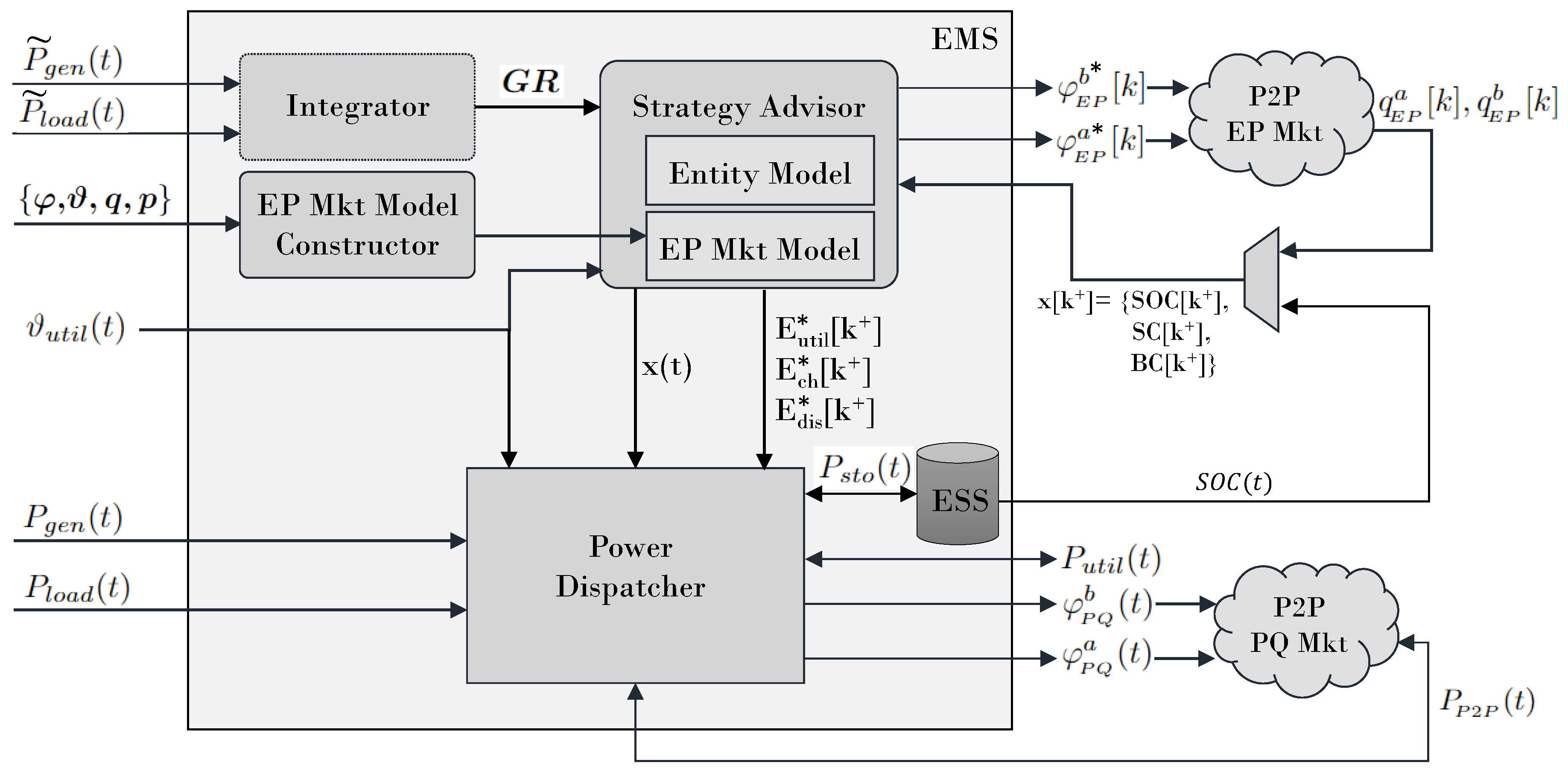
4. A Strategy Advisor Based on Model Predictive Control

The main objective of the Strategy Advisor is to meet the projected energy demand along the prediction horizon and to do so at the lowest possible cost. To this end, taking into account the existence and availability of the two markets, it generates an optimal dispatch plan that controls the energy flows for each of the sources that the entity has available. The vector of controllable variables is $\mathbf{u}=\{E_{util}\left[i\right],E_{ch}\left[i\right],E_{dis}\left[i\right],{\phi }^b\left[i\right],{\phi }^a\left[i\right]\},i\in \{{\tau }_k,{\tau }_{k+N-1}\}$. Its components correspond to the following energy quantities: $E_{util}\left[i\right]$ is the amount of energy to be consumed from the utility during the i-th period; $E_{ch}\left[i\right]$ and $E_{dis}\left[i\right]$ respectively correspond to the amount of energy to be charged or discharged from the ESS during i-th period; ${\phi }^b\left[i\right]$ is the amount of energy that the entity intends to buy at the i-th period, which will be bid in the market session held in $t={\tau }_i$; finally, ${\phi }^a\left[i\right]$ is the amount of energy that the entity attempts to sell in the i-th period, which will be asked in the market session held in $t={\tau }_i$. Therefore, the function corresponding to the cost of energy operation of the entity along a certain prediction horizon, N is:

$$\begin{array}{c}\mathcal{J}\left(\mathbf{x}\left[k\right]\right),\mathbf{u})=\sum _{i=k}^{k+N-1}{E}_{util}\left[i\right]·{\vartheta }_{util}\left[i\right]+{\phi }^b\left[i\right]·{\tilde{p}}_{{}_{EP}}\left[i\right]·(1-{\tilde{\ell }}^b\left[i\right])\hfill \\ \hfill -{\phi }^a\left[i\right]·{\tilde{p}}_{{}_{EP}}\left[i\right]·{\tilde{\ell }}^a\left[i\right]-({\lceil gr\left[i\right]\rceil }^{+}-E_{ch}\left[i\right])·{\tilde{p}}_{{}_{PQ}}\left[i\right]\end{array}$$

(8)

where the tilde (^˜) over a variable indicates it is a random variable. By multiplying the price ${\tilde{p}}_{{}_{EP}}$ by the buying liquidity complement $(1-{\tilde{\ell }}^b)$, the expected purchase prices of those market instants with low liquidity are artificially increased. Thus, during optimisation, agents acting as buyers will be more reluctant to plan their purchases at such market sessions. Alternatively, by multiplying the price ${\tilde{p}}_{{}_{EP}}$ by the selling liquidity ${\tilde{\ell }}^a$, the expected selling prices of those market instants with low liquidity are artificially lowered. Thus, during optimisation, agents acting as sellers will be more reluctant to plan their sales at such market sessions.

4.1. The Expected Value Problem

The economic objective function in (8) extends over a prediction horizon. Therefore, its elements refer to the future values of its inputs, which are the controllable variables, and to the future values of the state of the system and its outputs, which would result from the application of those inputs. Optimisation also depends on the forecast profiles of consumption, generation and prices for the two existing markets. These values, as already mentioned, are stochastic and therefore subject to uncertainty. A possible simplification consists in disregarding information on the uncertainty, taking a nominal scenario, and optimizing actions on the nominal scenario. As the common practice for defining a nominal scenario is to replace random variables by their expectation, the resulting problem is called the expected value problem, the solution of which constitutes a nominal plan [22]. At the next decision stage, the Strategy Advisor will recompute the plan by solving an updated expected value problem on a new nominal scenario that incorporates the observations of the current stage.

In this sense, the following formulation is deterministic, as it is based on nominal consumption, production and price profiles, without taking into account the aforementioned uncertainties. Specifically, within the optimisation, the market-related random variables ${\tilde{p}}_{{}_{EP}}\left[i\right],{\tilde{\ell }}^b\left[i\right],{\tilde{\ell }}^a\left[i\right],{\tilde{p}}_{{}_{PQ}}\left[i\right]$ are replaced by their respective expectations, ${\overline{p}}_{{}_{EP}}\left[i\right],{\overline{\ell }}^b\left[i\right],{\overline{\ell }}^a\left[i\right],{\overline{p}}_{{}_{PQ}}\left[i\right]$. Since there is no a priori statistical information available on market uncertainty, the expectation of variables in future instants is replaced by the average value of those variables in past isotemporal sessions (market sessions held at the same time period of the day but in previous days).

Thus, the optimisation problem to be solved in each $t={\tau }_k$ is the cost minimisation of the energy operation of the entity, which is defined by the formulation (9)–(23):

$$\begin{array}{ll}{\mathbf{u}}^{*}\left[i\right|k]=\underset{\begin{array}{c}{E}_{util}\left[i\right],E_{ch}\left[i\right],E_{dis}\left[i\right]\\ {\phi }^b\left[i\right],{\phi }^a\left[i\right]\end{array}}{\arg \min }& {\displaystyle \sum _{i=k}^{k+N-1}}{E}_{util}\left[i\right]·{\vartheta }_{util}\left[i\right]\\ & +{\phi }^b\left[i\right]·{\overline{p}}_{{}_{EP}}^b\left[i\right]·(1-{\overline{\ell }}^b\left[i\right])\\ & -{\phi }^a\left[i\right]·{\overline{p}}_{{}_{EP}}^a\left[i\right]·{\overline{\ell }}^a\left[i\right]\\ & -({\lceil gr\left[i\right]\rceil }^{+}-E_{ch}\left[i\right])·{\overline{p}}_{{}_{PQ}}\left[i\right]\end{array}$$

(9)

$$SOC[i+1]=SOC\left[i\right]-E_{dis}\left[i\right]-{\phi }^a\left[i\right]+E_{ch}\left[i\right]+min\{{\kappa }_e,BC\left[i\right]+{\phi }^b\left[i\right]\}$$

(10)

$$SC[i+1]=SC\left[i\right]+{\phi }^a\left[i\right]-min\{{\kappa }_e,SC\left[i\right]+{\phi }^a\left[i\right]\}$$

(11)

$$BC[i+1]=BC\left[i\right]+{\phi }^b\left[i\right]-min\{{\kappa }_e,BC\left[i\right]+{\phi }^b\left[i\right]\}$$

(12)

$${\tilde{E}}_{load}=E_{sc}\left[i\right]+E_{dis}\left[i\right]+E_{util}\left[i\right]$$

(13)

$$DO{D}_{max}\le SOC\left[i\right]\le 1$$

(14)

$$0\le E_{dis}\left[i\right]\le min\{{\kappa }_e,SOC\left[i\right]-DO{D}_{max}\}$$

(15)

$$0\le {\phi }^a\left[i\right]\le SOC\left[i\right]-DO{D}_{max}$$

(16)

$$0\le {\phi }^b\left[i\right]\le 1-SOC\left[i\right]$$

(17)

$$0\le E_{util}\left[i\right]\le {\tilde{E}}_{load}\left[i\right]$$

(18)

$$0\le E_{ch}\left[i\right]\le {\lceil gr\left[i\right]-E_{sc}\left[i\right]\rceil }^{+}$$

(19)

$${\phi }^a\left[i\right]·{\phi }^b\left[i\right]=0$$

(20)

$$SC\left[i\right]·{\phi }^b\left[i\right]=0$$

(21)

$$BC\left[i\right]·{\phi }^a\left[i\right]=0$$

(22)

$$0.4\le SOC[k+N-1]\le 0.6$$

(23)

where ${\kappa }_e$ is the energy transfer capacity of the entity’s converters (i.e., the maximum amount of energy that can be injected into/drained from the grid during a single period, and $DO{D}_{max}$ is the maximum allowable depth of discharge of the ESS. Please note that all variables are normalised with respect to the maximum storage capacity of the entity’s ESS, so that both states and control inputs are expressed in units of batteries.

Constraints (10) and (12) determine how the system evolves over time, while constraint (13) imposes that the expected load must be always meet, no matter which sources are used. The following assumptions has been considered in the controller as design criteria, which affect several constraints:

A.1. 

Following the prudence concept, quantities sold on the market are immediately deducted from the SOC, even though the physical transfer has not even begun. This avoids the possibility of selling already committed energy. On the contrary, the acquired energy is not assumed as immediately incorporated, but is added over time. This prevents the optimiser from allocating energy that is expected to be acquired in a future instant but will not be available until a later future instant (constraint (10)).

A.2. 

Once a purchase or sale agreement has been reached, the physical transfer of the energy associated with that transaction begins immediately and continues uninterruptedly until it is completed (constraints (11) and (12). In other words, transfers cannot be postponed.

A.3. 

Own production is dedicated primarily to self-consumption. Therefore, $E_{sc}\left[i\right]=min\{{\tilde{E}}_{gen}\left[i\right],{\tilde{E}}_{load}\left[i\right]\}$ is not a controllable variable but a parameter computed on the basis of the forecast generation and consumption.

A.4. 

Purchasing energy from the utility for later consumption is forbidden (constraint (18)). In other words, during periods of low tariff prices, the entity cannot acquire more energy than it needs from the utility in order to store it and consume it during periods of high tariffs.

A.5. 

In the same market session, each entity can only play one role, either buyer or seller (constraint (20)). Given that transfers must be started immediately after they are settled, an entity with unsatisfied sales commitments cannot go to the market as a buyer (constraint (21)); conversely, as long as it has unsatisfied buy commitments, an entity cannot go to the market as a seller (constraint (22)).

A.6. 

In the optimisation process, the strategic advisor assumes that future offers will be fully matched in the market (i.e., the optimiser assumes that $q^a\left[i\right]={\phi }^a\left[i\right]$ and $q^b\left[i\right]={\phi }^b\left[i\right]$). Immediately after the clearing of the k-th market session, the advisor already knows the real result of the offers shouted in that period. If the offers have not been matched, the available energy differs from that assumed in the optimal strategy profile, so it may be necessary to re-run the optimiser to adjust the values of $E_{util}\left[k\right],E_{ch}\left[k\right]$ and $E_{dis}\left[k\right]$. In any case, given that the optimiser is run before the next market session (for which the results of the immediately previous session are already available), the quantities actually offered, ${{\phi }^a}^{*}\left[k\right]$ and ${{\phi }^b}^{*}\left[k\right]$, are always the optimal ones based on the actual state at any given time.

4.2. Multiple Scenarios SMPC Approach (MS-SMPC)

From the point of view of each agent, both P2P markets are considered stochastic systems, since the outputs ($m=(q,p)$) for each one of the agent’s offers might be different for the same inputs ($\omega =\phi ,\vartheta )$), depending on the offers made by the other participant agents, which are considered an unknown disturbance. Scenario-based optimisation provides an intuitive way to approach the solution to the problem of stochastic optimisation. The idea behind this approach is to compute an optimal finite-horizon input sequence that is feasible under $N_s$ sampled ‘scenarios’ of the uncertainty, thus obtaining a certain level of robustness [23]. One of the advantages of this approach is that it does not assume a prior knowledge of the statistical properties that characterise uncertainty (e.g., a certain probability distribution function) as is generally required in stochastic optimisation. Each scenario consists of values for some or all of the stochastic processes that affect the system. Furthermore, it has been widely used for performing optimal power dispatch (e.g., [24]) and for optimal participation in energy markets [25]. In our case, only the stochasticity of the P2P markets’ prices is proposed to be addressed. Therefore, each scenario is a full horizon sample of the prices for the two markets,

$$\begin{array}{c}{\xi }_{\left(j\right)}\left[k\right]\stackrel{\mathrm{def}}{=}\{p_{{}_{E{P}_{\left(j\right)}}}\left[k\right],\dots ,p_{{}_{E{P}_{\left(j\right)}}}[k+N-1],{\ell }_{{}_{\left(j\right)}}^b\left[k\right],\dots ,{\ell }_{{}_{\left(j\right)}}^b[k+N-1],\hfill \\ \hfill {\ell }_{{}_{\left(j\right)}}^a\left[k\right],\dots ,{\ell }_{{}_{\left(j\right)}}^a\left[k\right],p_{{}_{P{Q}_{\left(j\right)}}}\left[k\right],\dots ,p_{{}_{P{Q}_{\left(j\right)}}}[k+N-1]\}\end{array}$$

(24)

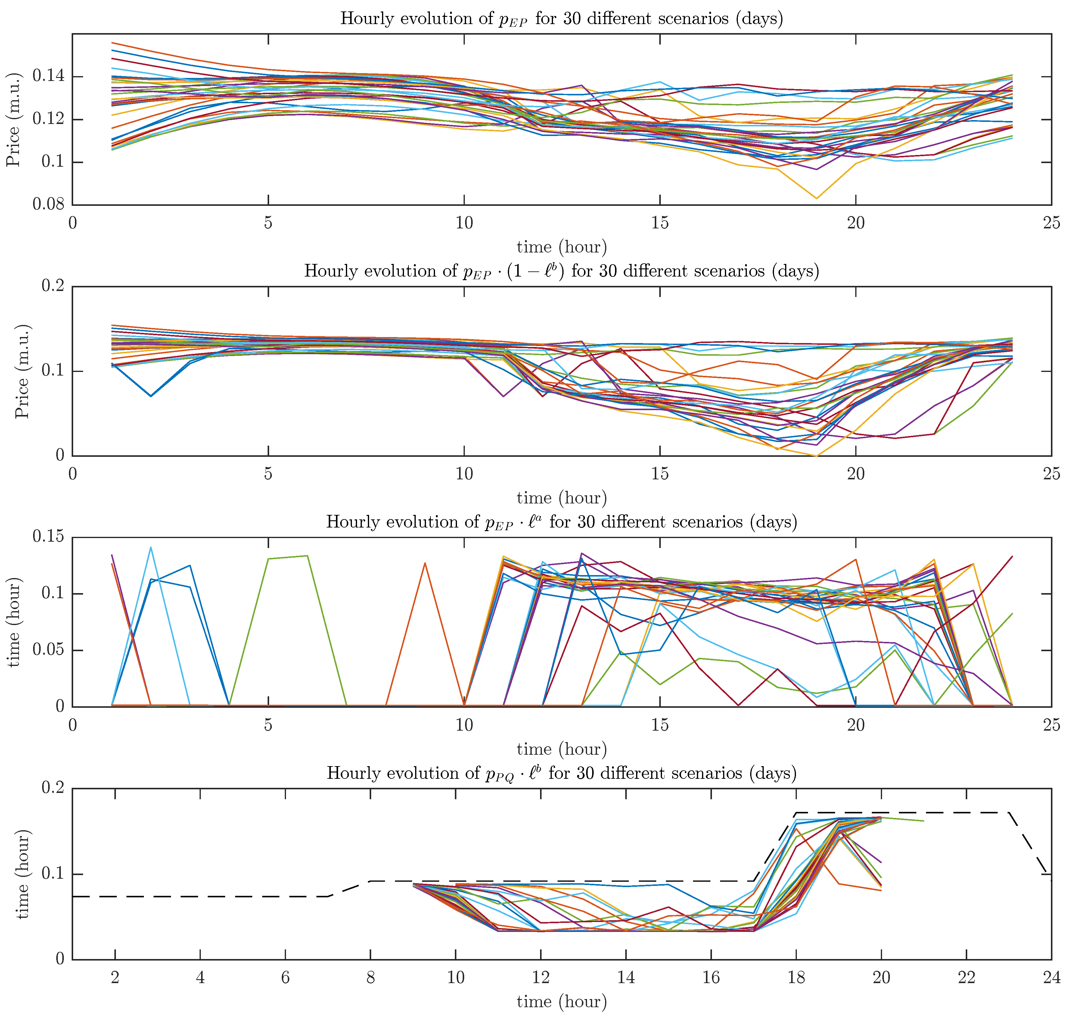
Specifically, within the optimisation, the market-related random variables ${\tilde{p}}_{{}_{EP}}\left[i\right]$, ${\tilde{\ell }}^b\left[i\right]$, ${\tilde{\ell }}^a\left[i\right]$ and ${\tilde{p}}_{{}_{PQ}}\left[i\right]$ are replaced by their corresponding values for each scenario, $p_{{}_{E{P}_{\left(j\right)}}}\left[i\right]$, ${\ell }_{{}_{\left(j\right)}}^b\left[i\right]$, ${\ell }_{{}_{\left(j\right)}}^a\left[i\right]$ and $p_{{}_{P{Q}_{\left(j\right)}}}\left[i\right]$.

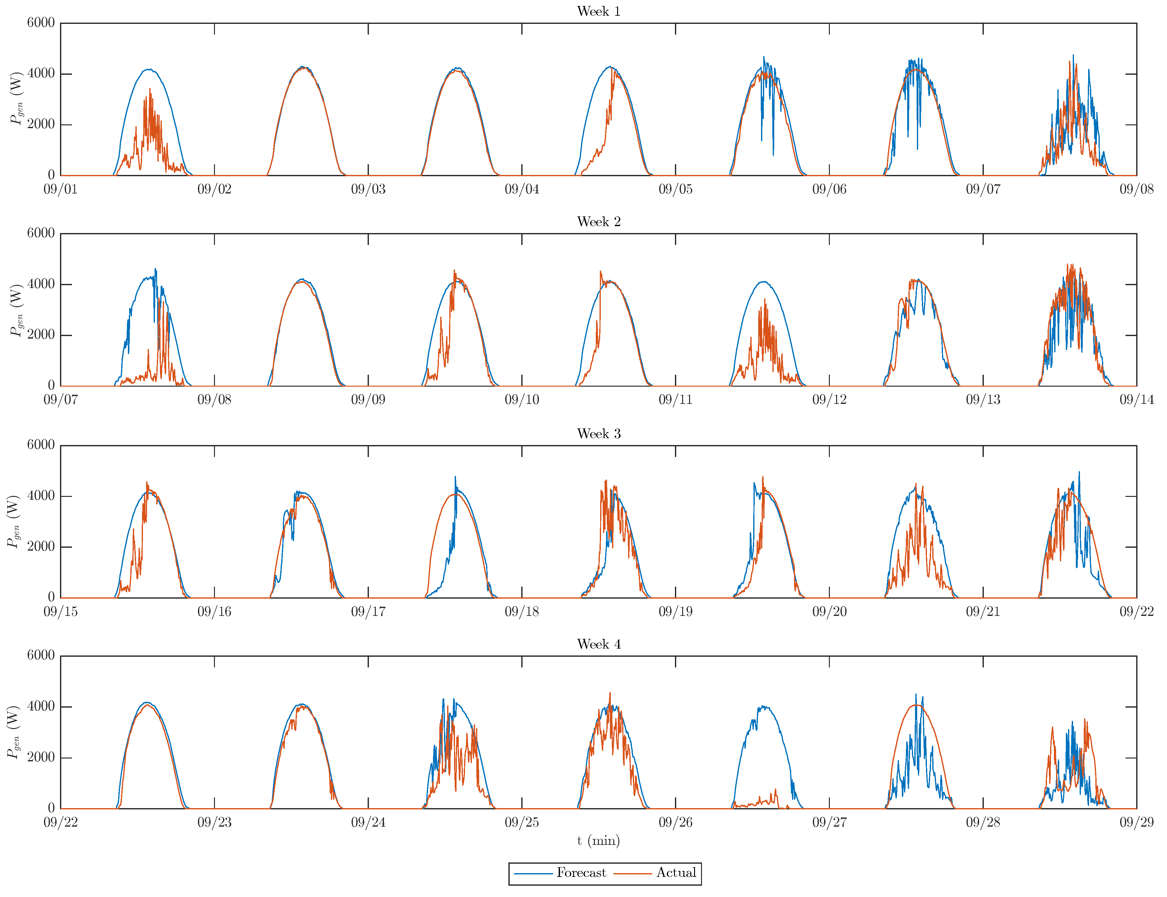
The offers that determine actual market parameters depend directly on the energy result expected by the different agents, which is given in turn by their consumption and generation forecasts. These predictions depend fundamentally on the climatology, and therefore present a significant level of correlation between consecutive days, as well as between identical days of previous years, provided that the typology of day (workable or weekend) is the same. Therefore, the approach proposed here to build the set of scenarios is to use the set of time series representing market realisations in past days (i.e., the evolution of the average prices and liquidities over similar periods of previous days). The Multiple Scenarios Stochastic MPC (MS-SMPC) problem then reads as follows:

$$\begin{array}{ll}{\mathbf{u}}^{*}\left[i\right|k]=\underset{\begin{array}{c}{E}_{util}\left[i\right],E_{ch}\left[i\right],E_{dis}\left[i\right]\\ {\phi }^b\left[i\right],{\phi }^a\left[i\right]\end{array}}{\arg \min }& {\displaystyle \sum _{j=1}^{N_s}}{\displaystyle \sum _{i=k}^{k+N-1}}{E}_{util}\left[i\right]·{\vartheta }_{util}\left[i\right]\\ & +{\phi }^b\left[i\right]·p_{{}_{E{P}_{\left(j\right)}}}^b\left[i\right]·(1-{\ell }_{\left(j\right)}^b\left[i\right])\\ & -{\phi }^a\left[i\right]·p_{{EP}_{\left(j\right)}}^a\left[i\right]·{\ell }_{\left(j\right)}^a\left[i\right]\\ & -({\lceil gr\left[i\right]\rceil }^{+}-E_{ch}\left[i\right])·{\overline{p}}_{{}_{PQ}}\left[i\right]\end{array}$$

(25)

$$SOC[i+1]=SOC\left[i\right]-E_{dis}\left[i\right]-{\phi }^a\left[i\right]+E_{ch}\left[i\right]+min\{{\kappa }_e,BC\left[i\right]+{\phi }^b\left[i\right]\}$$

(26)

$$SC[i+1]=SC\left[i\right]+{\phi }^a\left[i\right]-min\{{\kappa }_e,SC\left[i\right]+{\phi }^a\left[i\right]\}$$

(27)

$$BC[i+1]=BC\left[i\right]+{\phi }^b\left[i\right]-min\{{\kappa }_e,BC\left[i\right]+{\phi }^b\left[i\right]\}$$

(28)

$${\tilde{E}}_{load}=E_{sc}\left[i\right]+E_{dis}\left[i\right]+E_{util}\left[i\right]$$

(29)

$$DO{D}_{max}\le SOC\left[i\right]\le 1$$

(30)

$$0\le E_{dis}\left[i\right]\le min\{{\kappa }_e,SOC\left[i\right]-DO{D}_{max}\}$$

(31)

$$0\le {\phi }^a\left[i\right]\le SOC\left[i\right]-DO{D}_{max}$$

(32)

$$0\le {\phi }^b\left[i\right]\le 1-SOC\left[i\right]$$

(33)

$$0\le E_{util}\left[i\right]\le {\tilde{E}}_{load}\left[i\right]$$

(34)

$$0\le E_{ch}\left[i\right]\le {\lceil gr\left[i\right]-E_{sc}\left[i\right]\rceil }^{+}$$

(35)

$${\phi }^a\left[i\right]·{\phi }^b\left[i\right]=0$$

(36)

$$SC\left[i\right]·{\phi }^b\left[i\right]=0$$

(37)

$$BC\left[i\right]·{\phi }^a\left[i\right]=0$$

(38)

$$0.4\le SOC[k+N-1]\le 0.6$$

(39)

5. The Power Dispatcher

After solving the MS-SMPC formulated by Equations (25)–(39), since a receding-horizon strategy is used, only the first member of the optimal finite-horizon policy is kept and applied to the system, i.e., the SMPC control law is

$${\kappa }_{{}_{MSSMPC}}(\mathbf{x}\left[k\right],\xi \left[k\right])\stackrel{\mathrm{def}}{=}{u}^{*}\left[1\right|k]$$

(40)

5.1. Role Selection

Role Selection for the PQ-Market is performed based on the balance between generated power (if available) and consumed power. Peers with surplus go to the PQ-Market as sellers trying to trade that surplus whenever the SOC of their storage system is greater than a certain level $SO{C}_{Mkt}^{min}$. If the SOC is lower than this level, the surplus is used to charge that storage. Deficit peers go to the market as buyers trying to wipe out that deficit. As for the EP-Market, two possibilities arise, depending on whether the trading agent of the entity’s EMS implements an SA or not:

• A trading agent that does not have an SA, decides its role based only in its energy balance forecast. If $PD\left[{\tau }_k\right]<0$ the entity will play buyer, even if it has surplus for the immediate time slot. If $PD\left[{\tau }_k\right]=0\wedge PD\left[{\tau }_k\right]>0$ the entity will play seller, even if it has deficit for the immediate time slot (please remind that both $PD\left[k\right]$ and $PS\left[k\right]$ are variables that aggregate forecast over a prediction horizon).
• Role selection in trading agents who have a strategic advisor is an inherent result of the strategic optimisation itself. If ${\phi }^{b*}\left[1\right|{\tau }_k]>0$ the entity will play buyer in the immediate market session. Conversely, if ${\phi }^{a*}\left[1\right|{\tau }_k]>0$ the entity will play seller in the immediate market session. If ${\phi }^b\left[1\right|{\tau }_k]=0\wedge {\phi }^a\left[1\right|{\tau }_k]=0$ the entity remains idle, reserving itself for future and more potentially beneficial sessions. The possibility of ${\phi }^b\left[1\right|{\tau }_k]>0\wedge {\phi }^a\left[1\right|{\tau }_k]>0$ is avoided by the very definition of the optimiser’s constraints (20) and (36).

As mentioned before, the amounts ${{\phi }^a}^{*}\left[k\right]$ or ${{\phi }^b}^{*}\left[k\right]$ implicitly determine the role that the entity will adopt in the imminent market session (remember that only one of them can be non-zero). If the offers are matched, the optimal plan is still valid; otherwise, the optimiser must be run again to resolve the MS-SMPC replacing ${{\phi }^a}^{*}\left[k\right]$ by ${q^a}^{*}\left[k\right]$ and ${{\phi }^b}^{*}\left[k\right]$ by ${q^b}^{*}\left[k\right]$.

5.2. Demand Satisfaction

In either case, the optimal control variables $\{E_{util}^{*}\left[k^{+}\right],E_{ch}^{*}\left[k^{+}\right],E_{dis}^{*}\left[k^{+}\right]\}$ are sent as inputs to the power dispatcher (see Figure 1). The functions performed by this block are threefold: (i) to control the power flows to ensure that demand is met at all times, (ii) to maintain the state of charge of the Energy Storage System(s) within predefined safety levels, and (iii) to maximise, as far as possible, the profits obtained through the participation in the P2P market. Furthermore, those entities with Strategy Advisor use the continuous eP2P power quota market as a disturbance absorption mechanism, i.e., they go to this market only when the difference between the forecast consumption and generation profiles and the actual ones makes it impossible to operate following the optimal plan defined by the strategic advisor. Meanwhile, those entities whose EMS does not have the Strategy Advisor go to both the EP and the PQ Markets at any given time. In any case, the power demand satisfaction is driven at all times by Algorithm 1.

Algorithm 1 Demand Satisfaction Algorithm with Integrated Markets for peer k

1: Inputs

2: $\{E_{util}^{*}\left[k^{+}\right],E_{ch}^{*}\left[k^{+}\right],E_{dis}^{*}\left[k^{+}\right]\}$ Optimal Plan

3: $x\left(t\right)$ Current State

4: ${\vartheta }_{util}\left(t\right)$ Energy Price offered by the utility

5: Data

6: $SO{C}_{max}$ Maximum allowed ESS Level

7: $SO{C}_{min}$ Minimum allowed ESS Level

8: ${\kappa }_{stg}$ Maximum ESS charge/discharge power

9: Auxiliary

10: $\mathsf{\Phi }\left(t\right)$ Gross Power Balance: $\mathsf{\Phi }\left(t\right)\stackrel{\mathrm{def}}{=}{P}_{gen}\left(t\right)-P_{load}\left(t\right)$

11: $\mathsf{{\rm Y}}\left(t\right)$ Result After Rearrangement: $\mathsf{{\rm Y}}\left(t\right)\stackrel{\mathrm{def}}{=}{P}_{gen}\left(t\right)-P_{load}\left(t\right)+P_{{}_{P2P}}\left(t\right)$

12: $\mathsf{\Psi }\left(t\right)$ Net Power Balance: $\mathsf{\Psi }\left(t\right)\stackrel{\mathrm{def}}{=}{P}_{gen}\left(t\right)-P_{load}\left(t\right)+P_{{}_{P2P}}\left(t\right)+P_{sto}\left(t\right)$

13: $E_{util}^c\left(t\right)$ Accumulator of energy acquired from the utility during the k period

14: $E_{ch}^c\left(t\right)$ Accumulator of energy injected into the ESS during the k period

15: $E_{dis}^c\left(t\right)$ Accumulator of energy drained from the ESS during the k period

16: Result

17: $P_{sto}\left(t^{+}\right)$

18: $P_{util}\left(t^{+}\right)$

19: $SOC\left(t^{+}\right)$

20: while 1 do

21: if $\mathsf{{\rm Y}}\left(t\right)>0\wedge SOC\left(t\right)<SO{C}_{max}$ then

22:  ▹$P_{sc}\left(t\right)=P_{load}\left(t\right)$

23:  if $E_{ch}^{*}\left[k^{+}\right]\ge E_{ch}^c\left(t\right)$ then

24:   ▹ The optimal value of energy injected into the ESS has not yet been reached. Charge.

25:   $P_{ch}\left(t^{+}\right)\leftarrow min\{\mathsf{{\rm Y}}\left(t\right),{\kappa }_{stg}\}$

26:  else if $E_{ch}^{*}\left[k^{+}\right]<E_{ch}^c\left(t\right)$ then

27:   ▹ The optimal value of energy injected into the ESS has already been exceeded. Try to sell the surplus.

28:   $P_{ch}\left(t^{+}\right)\leftarrow 0$

29:   ${\phi }_{{}_{PQ}}^a\left(t\right)\leftarrow min\{\mathsf{{\rm Y}}\left(t\right),{\kappa }_{stg}\}$

30:  end if

31: else if $\mathsf{{\rm Y}}\left(t\right)<0$ then

32:  ▹$P_{sc}\left(t\right)=P_{gen}\left(t\right)$

33:  if $E_{dis}^{*}\left[k^{+}\right]\ge E_{dis}^c\left(t\right)$ then

34:   ▹ There is still room for discharge in this period. Drain the battery.

35:   $P_{dis}\left(t^{+}\right)\leftarrow -max\{\mathsf{{\rm Y}}\left(t\right),-{\kappa }_{stg}\}$

36:  else if $E_{dis}^{*}\left[k^{+}\right]<E_{dis}^c\left(t\right)$ then

37:   ▹ The ESS has already supplied all the energy planned for this period. Try to buy the deficit.

38:   $P_{dis}\left(t^{+}\right)\leftarrow 0$

39:   ${\phi }_{{}_{PQ}}^b\left(t\right)\leftarrow min\{-\mathsf{{\rm Y}}\left(t\right),{\kappa }_{stg}\}$

40:  end if

41: end if

42: Go to P2P PQ Market. $q_{{}_{PQ}}^b\left(t\right)$ and $q_{{}_{PQ}}^a\left(t\right)$ affect $P_{{}_{P2P}}\left(t\right)$

43: Recompute $\mathsf{\Psi }\left(t\right)$ with the updated value $P_{{}_{P2P}}\left(t\right)$.

44: if $\mathsf{\Psi }\left(t\right)>0$ then                    ▹ Could not sell all the excess.

45:  if $SOC\left(t\right)<1$ then                 ▹ Store the remaining surplus

46:   $P_{ch}\left(t^{+}\right)\leftarrow min\{\mathsf{\Psi }\left(t\right),{\kappa }_{stg}\}$

47:  else if $SOC\left(t\right)=1$ then            ▹ Sell remaining surplus to the utility

48:   $P_{util}\left(t^{+}\right)\leftarrow -\mathsf{\Psi }\left(t\right)$

49:  end if

50: else if $\mathsf{\Psi }\left(t\right)<0$ then                ▹ Could not purchase all the defitit.

51:  $P_{util}\left(t^{+}\right)\leftarrow -\mathsf{\Psi }\left(t\right)$

52: else

53:  ▹$\mathsf{\Psi }\left(t\right)=0$ Perfect Balance

54:  $P_{util}\left(t^{+}\right)\leftarrow 0$

55: end if

56: $E_{ch}\left(t\right)\leftarrow min({\int }_{\mathsf{\Delta }t\to 0}{P}_{ch}\left(\tau \right)d\tau ,SO{C}_{max}-SOC\left(t\right)))$

57: $E_{dis}\left(t\right)\leftarrow max({\int }_{\mathsf{\Delta }t\to 0}-P_{dis}\left(\tau \right)d\tau ,SOC\left(t\right)-SO{C}_{min}))$

58: $E_{ch}^c\left(t^{+}\right)\leftarrow E_{ch}^c\left(t\right)+E_{ch}\left(t\right)$

59: $E_{dis}^c\left(t^{+}\right)\leftarrow E_{dis}^c\left(t\right)+E_{dis}\left(t\right)$

60: $E_{util}^c\left(t^{+}\right)\leftarrow E_{util}^c\left(t\right)+{\int }_{\mathsf{\Delta }t\to 0}max\{0,P_{util}\left(\tau \right)d\tau \}$

61: $SOC\left(t^{+}\right)=SOC\left(t\right)+E_{ch}\left(t\right)+E_{dis}\left(t\right)$

62: end while

6. Case Study

6.1. Description

In this case example the entities are a group $\mathcal{H}$ of 100 houses within the same neighbourhood in the city of Córdoba (Spain). Some of these houses ($P{V}_{pen}=45\%$) are supposed to have photovoltaic (PV) generation systems. There are three possible installed PV powers, $P_{phv}\in \{1,3,5\}$ kWp, and each of them has an associated ESS of adequate capacity, $B_{max}\in \{2.5,5,7\}$ kWh respectively. Houses with no PV-installation still have an ESS of $B_{max}=10$ kWh to be able to participate in the EP-Market. Among the 100 houses, $S{A}_{pen}=10\%$ (10 Houses) are randomly selected which form the control set, ${\mathcal{H}}_c$. These houses are replicated twice, giving rise to three sets:

• Set NoStrat, (${\mathcal{H}}_c$): Houses without Strategy Advisor.
• Set Strat-NonSto, (${\mathcal{H}}_{ns}$): Houses with Strategy Advisor based on expected value scenario according to optimisation problem (9).
• Set Strat-Sto, (${\mathcal{H}}_s$): Houses with MS-SMPC-based Strategy Advisor according to optimisation problem (25).

The ${\mathcal{H}}_{ns}$ and ${\mathcal{H}}_s$ resulting sets (20 houses) are simulated together with the remaining $\mathcal{H}$ houses of the original population, which already include ${\mathcal{H}}_c$, giving rise to a total population of $n_{{}_{\mathcal{H}}}$ = 120 houses. All houses simultaneously participate in the two different markets. The first one is a PQ-Market similar to the one introduced in [20]. The second one is an hourly EP-Market. The main parameters of both markets are displayed in

Table 2. Main parameters of integrated markets.

	PQ-Market	EP-Market
Type	CDA	DDA
$\mathsf{\Delta }\mathbf{T}$	1 min a	60 min
${\mathbf{q}}_{\mathbf{min}}$	0.1 (kWmin)	0.25 (kWh)
${\mathbf{q}}_{\mathbf{max}}$	3.3 (kWmin)	1 (kWh)

^a Equal to the temporal resolution of the energy operation simulation, thus mimicking a continuous market.

. The EMS of all houses incorporates two trading agents, one per each market.

6.1.1. Scenario Generation

To generate the scenarios (price evolution and market liquidity profiles), a full month (30 days) of operation of 100 houses (all without Strategy Advisor) was simulated. These simulations assumed that each agent perfectly knows its generation and consumption profiles, obtained from [26], so that offers (and thus prices) reflect the real energy needs/excess of the traders within the simulated days. The results are shown in Figure 3. In a real application case, the equivalent of these scenarios obtained by simulation would be the historical data profiles obtained either from similar days in previous years or from the days immediately preceding the current operation day, or from a combination of both.

6.1.2. Operation Costs and Final Stock Valuation

In this case study, the net cost of energy for the i-th house over a certain period of time ($T=[t_i,t_f]$) can be calculated as:

$${\mathsf{\Phi }}^i\left(T\right)={\mathsf{\Phi }}_{util}^i\left(T\right)+{\mathsf{\Phi }}_c^i\left(T\right)+{\mathsf{\Phi }}_{{}_{EP}}^i\left(T\right)+{\mathsf{\Phi }}_{{}_{PQ}}^i\left(T\right)$$

(41)

where

$$\begin{array}{cc}\hfill {\mathsf{\Phi }}_{util}^i\left(T\right)& =\sum _{\forall t\in T}^{}{E}_{{}_{util}}^i\left(t\right)·\vartheta \left(t\right)\hfill \end{array}$$

(42)

$$\begin{array}{cc}\hfill {\mathsf{\Phi }}_c^i\left(T\right)& =E_{{}_c}^i\left(T\right)·\overline{\vartheta }\hfill \end{array}$$

(43)

$$\begin{array}{cc}\hfill {\mathsf{\Phi }}_{{}_{EP}}^i\left(T\right)& =\sum _{\forall {\omega }_e\in {\mathsf{\Omega }}_i^{ep}}^{}{\mathcal{A}}_{{\omega }_e}^i\left(T\right)\hfill \end{array}$$

(44)

$$\begin{array}{cc}\hfill {\mathsf{\Phi }}_{{}_{PQ}}^i\left(T\right)& =\sum _{\forall {\omega }_p\in {\mathsf{\Omega }}_i^{pq}}^{}{\mathcal{A}}_{{\omega }_p}^i\left(T\right)\hfill \end{array}$$

(45)

being ${\mathcal{A}}_{{\omega }_e}^i\left(T\right)$ the amount of money corresponding to each energy package transaction ${\omega }_e$ in the set ${\mathsf{\Omega }}_i^{ep}$ of all eP2P transactions dealt by house i at the EP-Market within T, and ${\mathcal{A}}_{{\omega }_p}^i\left(T\right)$ the amount of money corresponding to each power quota transaction ${\omega }_p$ in the set ${\mathsf{\Omega }}_i^{pq}$ of all eP2P transactions dealt by house i at the PQ-Market within T:

$${\mathcal{A}}_{\omega }=q_{\omega }·p_{\omega }$$

(46)

where $q_{\omega }$ is the traded quantity and $p_{\omega }$ is the unit price of the agreed transaction.

Equation (41) is the sum of the cost of energy purchased from the utility (42), plus the revenue of energy compensated by the utility at a price equal to the Voluntary Price for the Small Consumer (VPSC), ${\overline{\vartheta }}_c$, (43), plus the result of trading in the EP-Market (44), plus the result of trading in the PQ-Market (45). A Net Purchase and Sell Scheme (NPSS) is followed here to calculate the amount of compensated energy. Under this arrangement, two uni-directional meters are installed: one records electricity drawn from the grid, and the other records excess electricity generated and fed back into the grid. Prosumers pay retail rate for the electricity they use, and the DSO purchases their excess generation at its avoided cost (wholesale rate), up to the amount of consumed energy, so that prosumers may have zero energy cost with respect to the utility, but no positive balance. By convention, costs have a negative sign, while revenues have a positive sign. In addition, and although it is not directly part of the operating result, a way of computing the value of the energy stored at the end of the operating period in the ESS of each house is necessary:

$${\mathsf{\Phi }}_{B_f}^i=B_r^i\left(t_f\right)·{\lambda }^i\left(t_f\right)$$

(47)

where $t_f$ is the final instant of the period of comparison and ${\lambda }^i\left(t_f\right)$ is the private valuation of energy for house i in $t=t_f$ according to (6).

6.1.3. Comparative Indicators

The comparison is then made between the energy operation results of ${\mathcal{H}}_c$ and those of ${\mathcal{H}}_{ns}$ and ${\mathcal{H}}_s$. The following indicators can be computed to compare the operation performance of two sets of houses (${\mathcal{H}}_a$ and ${\mathcal{H}}_b$) (Energy Result Comparator, EP-Market Result Comparator, PQ-Market Result Comparator, Renewable Energy Use Comparator and Battery Usage Comparator) and are defined below:

$$\mathsf{\Delta }\mathsf{\Phi }\left(T\right)=\frac{{⌈{\mathsf{\Phi }}_{B_f}^a-{\mathsf{\Phi }}_{B_f}^b⌉}^{+}+{\displaystyle \sum _{\forall h\in {\mathcal{H}}_a}}{\mathsf{\Phi }}^h\left(T\right)}{{⌈{\mathsf{\Phi }}_{B_f}^b-{\mathsf{\Phi }}_{B_f}^a⌉}^{+}+{\displaystyle \sum _{\forall h\in {\mathcal{H}}_b}}{\mathsf{\Phi }}^h\left(T\right)}-1$$

(48)

$$\mathsf{\Delta }R{W}_{use}\left(T\right)=\frac{{\displaystyle \sum _{\forall h\in {\mathcal{H}}_a}}R{W}^h\left(T\right)}{{\displaystyle \sum _{\forall h\in \mathcal{H}}}R{W}^h\left(T\right)}-1$$

(49)

$$\mathsf{\Delta }{B}_{use}\left(T\right)=\frac{{\displaystyle \sum _{\forall h\in {\mathcal{H}}_a}}{B}^h\left(T\right)}{{\displaystyle \sum _{\forall h\in {\mathcal{H}}_b}}{B}^h\left(T\right)}-1$$

(50)

6.2. Tests and Results

Testing the effects of the MS-SMPC-based Strategy Advisor is a complicated task. First, because the number of optimisation variables grows very fast as the length of the prediction horizon is increased. In turn, the more optimisation variables the problem has, the number $N_S$ of different scenarios needed to reach a certain level of confidence also increases [27].

Additionally, since the experiments are basically agent-based simulations, it is difficult to guarantee common conditions for entities with/without (non-)stochastic Strategy Advisor. For each element $h_c\in {\mathcal{H}}_c$, two identical reproductions are created, $h_{ns}\in {\mathcal{H}}_{ns}$ and $h_s\in {\mathcal{H}}_s$. These three elements have exactly the same consumption and generation profiles, and in addition, the parameters of their respective agents are also identical, including those that drive price adaptation and private valuation determination. Therefore, the price evolution of bids and asks is the same for the three entities. What changes between them, and in fact is the origin of the performance variability, is the sequence of roles adopted in the market. Entities in ${\mathcal{H}}_c$ adopt one or another role in an obtuse manner, without considering the plausible evolution of the market. In contrast, the objective of the Strategy Advisor is to steer the role selection and the temporal allocation of offered energy quantities so that the entity takes advantage of those hourly sessions with the highest expected revenue.

Each simulation covers a whole week of energy operation during the month of September. To check whether in the presence of uncertainty the stochastic strategy advisor is capable of obtaining better results than the one based on the nominal scenario, it is necessary to simulate prediction errors. For this, the agents are simulated using the real generation profile, while their forecast profile is randomly picked among the pool of daily generation profiles corresponding to the 30 days of September. Figure 4 shows the forecast and actual PhV power generation profiles for each week, in which it can be seen how both accurate and imprecise forecasting are artificially simulated.

Table 3. Summary of energy interactions with the utility (purchased energy).

	Utility Import Interactions
September	${\mathit{E}}_{\mathit{util}}$ (kWh)			${\mathsf{\Phi }}_{\mathit{util}}$ (€)			${\overline{\mathit{\vartheta }}}_{\mathit{util}}$ (c€/kWh)
	${\mathcal{H}}_{\mathit{c}}$	${\mathcal{H}}_{\mathit{ns}}$	${\mathcal{H}}_{\mathit{s}}$	${\mathcal{H}}_{\mathit{c}}$	${\mathcal{H}}_{\mathit{ns}}$	${\mathcal{H}}_{\mathit{s}}$	${\mathcal{H}}_{\mathit{c}}$	${\mathcal{H}}_{\mathit{ns}}$	${\mathcal{H}}_{\mathit{s}}$
Week 1	329.42	296.49	286.05	−38.9	−35.59	−34.54	−11.81	−12	−12.07
Week 2	372.57	342.33	321.58	−42.75	−39.78	−37.29	−11.47	−11.62	−11.6
Week 3	320.12	256.58	253.01	−36.16	−28.86	−28.23	−11.29	−11.25	−11.15
Week 4	355.48	325.24	322.88	−41.1	−38.18	−38.04	−11.56	−11.74	−11.78

,

Table 4. Summary of energy interactions with the utility (compensated energy).

	Utility Export Interactions
September	${\mathit{E}}_{\mathit{c}}$ (kWh)			${\mathsf{\Phi }}_{\mathit{c}}$ (€)
	${\mathcal{H}}_{\mathit{c}}$	${\mathcal{H}}_{\mathit{ns}}$	${\mathcal{H}}_{\mathit{s}}$	${\mathcal{H}}_{\mathit{c}}$	${\mathcal{H}}_{\mathit{ns}}$	${\mathcal{H}}_{\mathit{s}}$
Week 1	21.97	45.79	50.17	1.10	2.29	2.51
Week 2	13.56	39.76	42.26	0.69	1.99	2.11
Week 3	22.15	34.42	30.21	1.11	1.72	1.51
Week 4	33.25	49.44	50.28	1.66	2.47	2.51

,

Table 5. P2P energy-package market buying interactions.

P2P EP-Market Buying Interactions
September	${\mathit{E}}_{\mathit{ep}}^{\mathit{b}}$ (kWh)			${\mathsf{\Phi }}_{\mathit{ep}}^{\mathit{b}}$ (€)			${\overline{\mathit{\vartheta }}}_{\mathit{ep}}^{\mathit{b}}$ (c€/kWh)
	${\mathcal{H}}_{\mathit{c}}$	${\mathcal{H}}_{\mathit{ns}}$	${\mathcal{H}}_{\mathit{s}}$	${\mathcal{H}}_{\mathit{c}}$	${\mathcal{H}}_{\mathit{ns}}$	${\mathcal{H}}_{\mathit{s}}$	${\mathcal{H}}_{\mathit{c}}$	${\mathcal{H}}_{\mathit{ns}}$	${\mathcal{H}}_{\mathit{s}}$
Week 1	79.45	90.25	99.59	−9.07	−10.22	−11.27	−11.42	−11.33	−11.32
Week 2	78.55	73.05	81.47	−9	−8.33	−9.3	−11.46	−11.4	−11.42
Week 3	78.65	78.7	89.56	−9.13	−9.05	−10.35	−11.61	−11.5	−11.56
Week 4	73.1	82.08	84.57	−8.05	−8.35	−8.67	−11.01	−10.18	−10.25

,

Table 6. P2P energy-package market selling interactions.

P2P EP-Market Selling Interactions
September	${\mathit{E}}_{\mathit{ep}}^{\mathit{s}}$ (kWh)			${\mathsf{\Phi }}_{\mathit{ep}}^{\mathit{s}}$ (€)			${\overline{\mathit{\vartheta }}}_{\mathit{ep}}^{\mathit{s}}$ (c€/kWh)
	${\mathcal{H}}_{\mathit{c}}$	${\mathcal{H}}_{\mathit{ns}}$	${\mathcal{H}}_{\mathit{s}}$	${\mathcal{H}}_{\mathit{c}}$	${\mathcal{H}}_{\mathit{ns}}$	${\mathcal{H}}_{\mathit{s}}$	${\mathcal{H}}_{\mathit{c}}$	${\mathcal{H}}_{\mathit{ns}}$	${\mathcal{H}}_{\mathit{s}}$
Week 1	150.27	176.28	176.35	17.16	20.45	20.47	11.41	11.60	11.61
Week 2	127.79	152.77	148.49	14.72	17.89	17.41	11.51	11.71	11.72
Week 3	157.37	173.89	172.56	18.19	18.19	20.22	11.56	11.71	11.72
Week 4	118.34	135.33	141.59	13.05	15.01	15.69	11.03	11.09	11.08

,

Table 7. P2P power quota market interactions.

P2P PQ-Market Buying Interactions
September	${\mathit{E}}_{\mathit{pq}}^{\mathit{b}}$ (kWh)			${\mathsf{\Phi }}_{\mathit{pq}}^{\mathit{b}}$ (€)			${\overline{\mathit{\vartheta }}}_{\mathit{pq}}^{\mathit{b}}$ (c€/kWh)
	${\mathcal{H}}_{\mathit{c}}$	${\mathcal{H}}_{\mathit{ns}}$	${\mathcal{H}}_{\mathit{s}}$	${\mathcal{H}}_{\mathit{c}}$	${\mathcal{H}}_{\mathit{ns}}$	${\mathcal{H}}_{\mathit{s}}$	${\mathcal{H}}_{\mathit{c}}$	${\mathcal{H}}_{\mathit{ns}}$	${\mathcal{H}}_{\mathit{s}}$
Week 1	146.61	89.47	92.9	−7.26	−4.24	−4.21	−4.95	−4.74	−4.54
Week 2	135.24	87.49	98.88	−7.36	−4.10	−4.74	−5.44	−4.69	−4.79
Week 3	129.78	99.38	90.35	−6.33	−4.50	−4.03	−4.88	−4.53	−4.46
Week 4	123.74	75.14	76.72	−6.18	−3.49	−3.46	−4.99	−4.65	−4.52

,

Table 8. P2P power-quota market selling interactions.

P2P PQ-Market Interactions
September	${\mathit{E}}_{\mathit{pq}}^{\mathit{s}}$ (kWh)			${\mathsf{\Phi }}_{\mathit{pq}}^{\mathit{s}}$ (€)			${\overline{\mathit{\vartheta }}}_{\mathit{pq}}^{\mathit{s}}$ (c€/kWh)
	${\mathcal{H}}_{\mathit{c}}$	${\mathcal{H}}_{\mathit{ns}}$	${\mathcal{H}}_{\mathit{s}}$	${\mathcal{H}}_{\mathit{c}}$	${\mathcal{H}}_{\mathit{ns}}$	${\mathcal{H}}_{\mathit{s}}$	${\mathcal{H}}_{\mathit{c}}$	${\mathcal{H}}_{\mathit{ns}}$	${\mathcal{H}}_{\mathit{s}}$
Week 1	301.58	153.05	152.49	14.13	7.61	7.79	4.69	4.97	5.11
Week 2	264.98	114.24	112.71	12.82	6.45	6.06	4.84	5.65	5.38
Week 3	283.68	139.70	140.31	13.10	7.22	6.94	4.62	5.17	4.95
Week 4	235.54	115.71	115.59	10.49	5.57	5.91	4.45	4.81	5.11

and

Table 9. Valuation of final stock of stored energy.

Valuation of Final Storage
September	${\mathit{B}}_{\mathit{f}}$ (kWh)			${\mathsf{\Phi }}_{{\mathit{B}}_{\mathit{f}}}$ (€)
	${\mathcal{H}}_{\mathit{c}}$	${\mathcal{H}}_{\mathit{ns}}$	${\mathcal{H}}_{\mathit{s}}$	${\mathcal{H}}_{\mathit{c}}$	${\mathcal{H}}_{\mathit{ns}}$	${\mathcal{H}}_{\mathit{s}}$
Week 1	22.66	22.12	21.65	2.73	2.65	2.59
Week 2	31.03	25.55	26.72	3.76	3.08	3.24
Week 3	24.85	27.45	26.61	2.87	3.19	3.10
Week 4	26.77	25.37	25.15	3.10	2.96	2.94

show the results of the simulations for each of the addends that allow to compute the economic result derived from the energy operation (Equations (41) and (47)) of the three replicated sets.

Figure 5, Figure 6, Figure 7 and Figure 8 are the radar plots [28] of Weeks 1–4, where the different components of the economic result are displayed along with the total results, $\mathsf{\Phi }(T=1\mathrm{week})$, themselves.

Finally,

Table 10. Comparative indicators.

September	$\mathsf{\Delta }{\mathsf{\Phi }}_{\mathit{cost}}$ (%)		$\mathsf{\Delta }{\mathit{RW}}_{\mathit{use}}$ (%)		$\mathsf{\Delta }{\mathit{B}}_{\mathit{use}}$ (%)		${\mathsf{\Gamma }}_{{}_{\mathit{RW}}}$ (%)
	${\mathcal{H}}_{\mathit{ns}}$	${\mathcal{H}}_{\mathit{s}}$	${\mathcal{H}}_{\mathit{ns}}$	${\mathcal{H}}_{\mathit{s}}$	${\mathcal{H}}_{\mathit{ns}}$	${\mathcal{H}}_{\mathit{s}}$	${\mathcal{H}}_{\mathit{ns}}$	${\mathcal{H}}_{\mathit{s}}$
Week 1	−13.46	−15.19	−3.05	−2.89	+59.89	+61.46	96.95	97.11
Week 2	−14.33	−15.22	−3.47	−3.66	+66.53	+69.36	96.53	96.34
Week 3	−33.46	−28.62	−2.76	−3.37	+64.87	+68.52	97.24	96.63
Week 4	−10.04	−12.99	−2.72	−1.71	+55.74	+57.97	97.28	98.29

shows the comparative indicators with respect to the performance of the set of houses without SA (${\mathcal{H}}_c$)) for the set of houses with Nominal MPC-based SA (${\mathcal{H}}_{ns}$) and for the set of houses with MS-SMPC-based SA (${\mathcal{H}}_s$).

7. Discussion

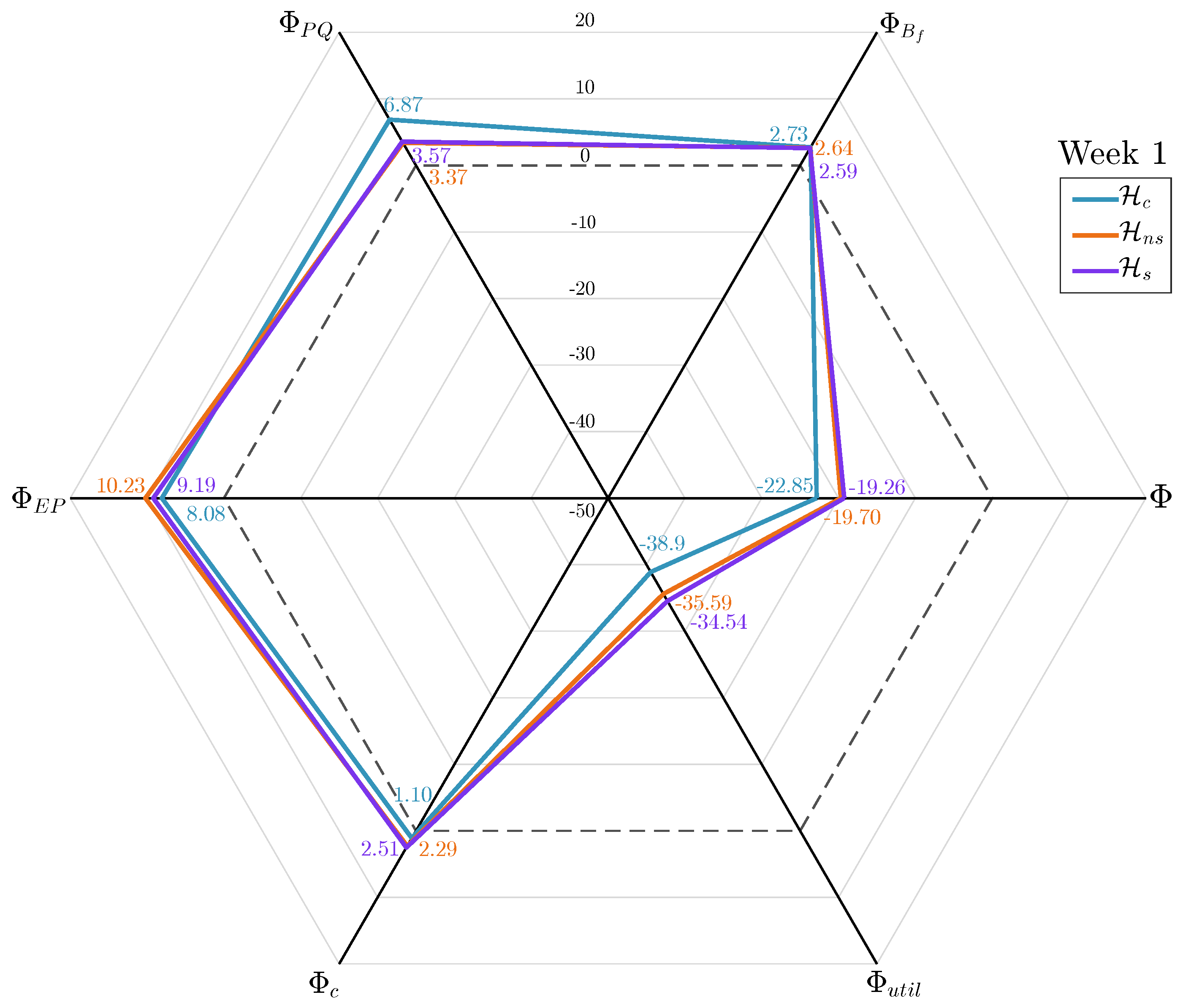
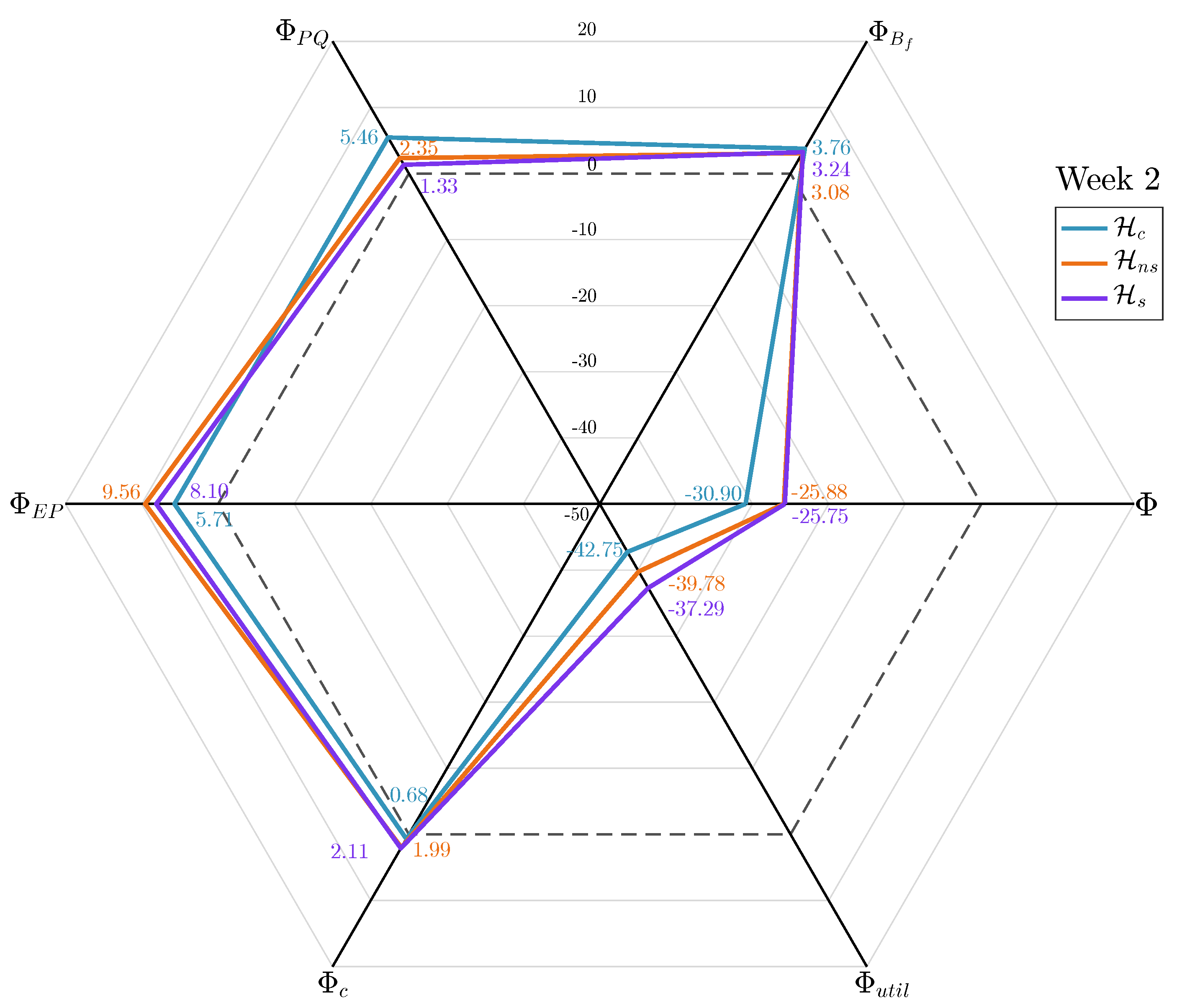
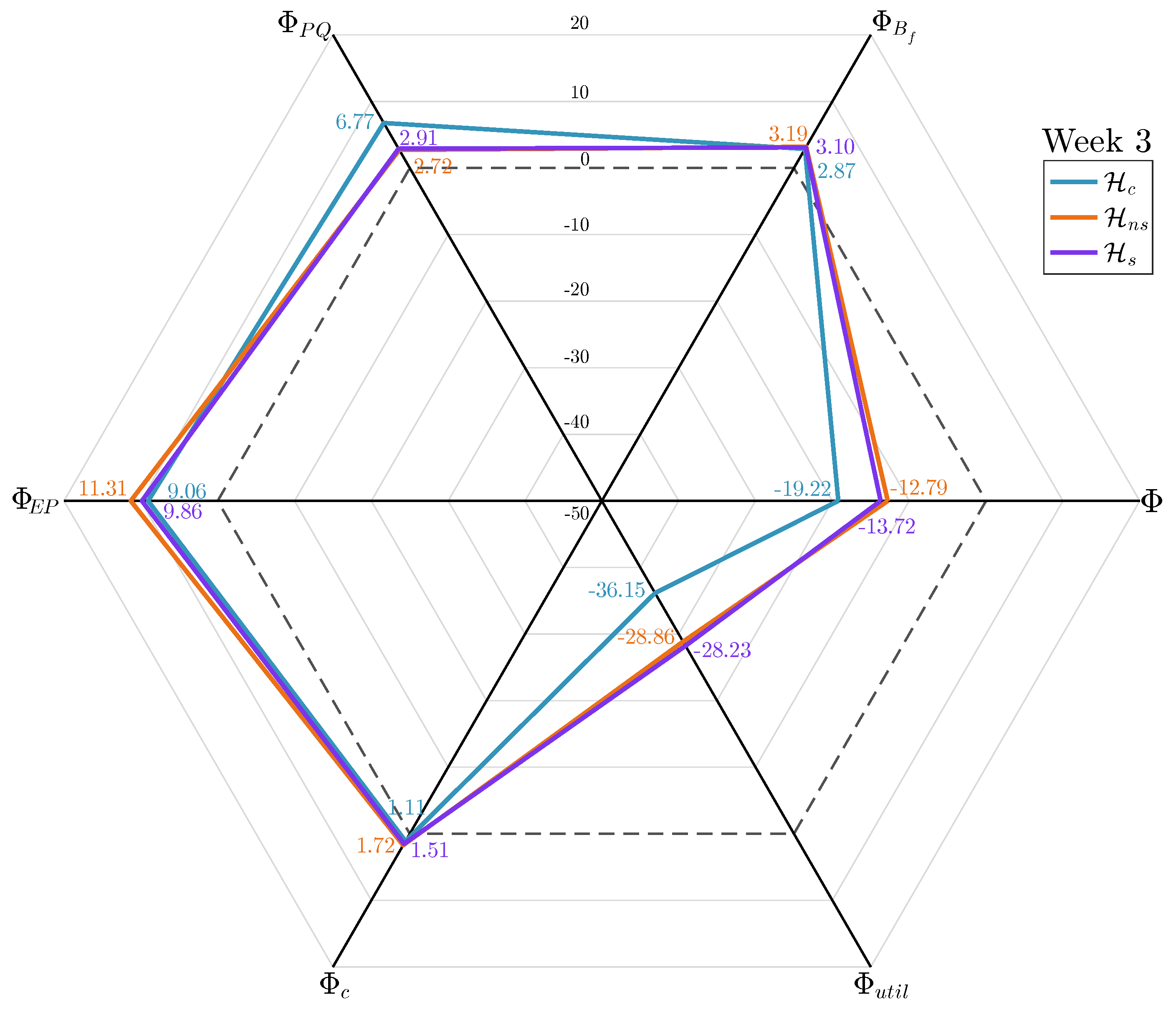
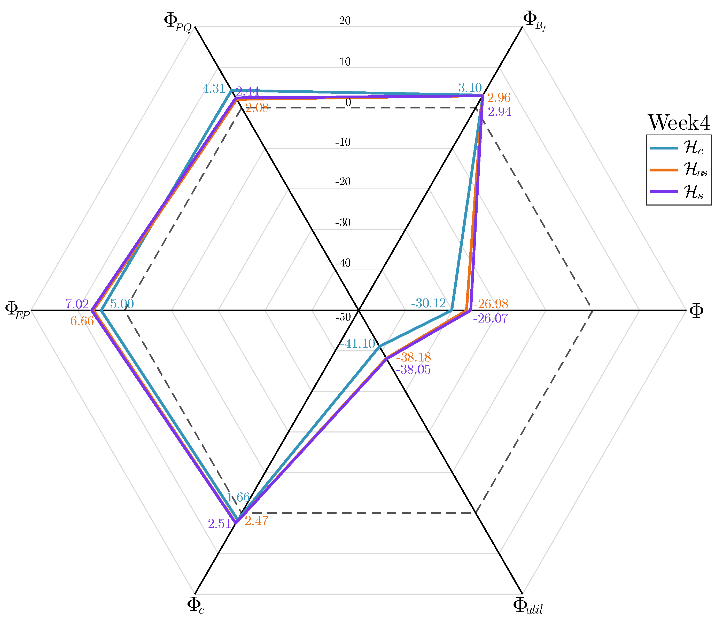
This article proposes the simultaneous participation of energy traders in two energy markets which run in parallel while being executed simultaneously. The discrete EP-Market acts as a futures market, allowing traders to purchase/sell energy packages in advance of the occurrence of a forecast deficit. The continuous PQ-Market acts as a spot market, in which power quotas are negotiated to balance deficits and excesses instantly. To allow this simultaneous participation, a specifically designed EMS is required to allow the automation of the procedures for determining private valuation, price adaptation and role selection for each of the two markets. Entities with an excess of energy generation act as sellers, and have the option of either selling as much as they can as soon as possible (in the immediately following market moments) or offering the aforementioned excess at certain future market moments where the price obtained is historically more advantageous. They must also decide on the quantities to be offered in the discrete market, taking into account that the stock sold in the time-ahead market is no longer available for sale in the real-time market. On the other hand, entities that foresee having an energy deficit (those whose expected consumption is greater than their foreseen generation) have to decide whether to try to anticipating it by obtaining energy packages in the discrete market, which is generally more expensive but less volatile, or to risk trying to cancel their deficit in the continuous market of power quotas, which is generally cheaper but less liquid. In this sense, the proposed EMS can incorporate the strategy advice functionality, consisting on the determination of the optimal energy operation profile and encompasses the storage utilisation, the energy acquisition from the power grid and the interactions foreseen in the two eP2P markets. This article proposes a possible implementation of this Strategy Advisor, based on MPC, including two variants, one based on a single nominal scenario, and the other based on SMPC, which optimises contemplating multiple scenarios. Simulations carried out on the case study show that both variants offer an improvement in economic performance of between 10% and 30% compared to the case of not using a SA. Furthermore, the MS-SMPC-based variant generally performs slightly better than the nominal variant, as it contemplates more possible market price evolution profiles (derived from different PV generation scenarios), although to state this conclusively it would be necessary to make a deeper statistical analysis which is beyond the scope of this article. These savings are mainly achieved by buying less energy from the grid and replacing it with cheaper energy, either previously bought and stored or bought instantaneously; and by selling a greater portion of the surplus energy in market sessions where the price is higher. But it’s not all advantages. This improvement is also achieved through an intensification of the use of storage systems, which could lead to a reduction in their lifespan. The translation of depreciation costs into the calculation of energy operating costs is an open issue, both in terms of the selection of the usage level indicator and in terms of the monetisation of such usage.