A New Cross-Correlation Algorithm Based on Distance for Improving Localization Accuracy of Partial Discharge in Cables Lines

Abstract

Locating the partial discharge (PD) source is one of the most effective means to locate local defects in power cable lines. The sampling rate and the frequency-dependent characteristic of phase velocity have an obvious influence on localization accuracy based on the times of arrival (TOA) evaluation algorithm. In this paper, we present a cross-correlation algorithm based on propagation distance to locate the PD source in cable lines. First, we introduce the basic principle of the cross-correlation function of propagation distance. Then we verify the proposed method through a computer simulation model and investigate the influences of propagation distance, sampling rate, and noise on localization accuracy. Finally, we perform PD location experiments on two 250 m 10 kV XLPE power cables using the oscillation wave test system. The simulation and experiment results indicate that compared with traditional TOA evaluation methods, the proposed method has superior locating precision.

1. Introduction

Power cables have been extensively used in urban power grids because of their reliable electrical and mechanical properties. In normal operations, partial defects can occur in power cable lines due to long-term environmental, mechanical, and electrical stresses. The further degradation of cable defects can lead to partial discharge (PD) [1,2]. It is difficult to find the location of the defects in long underground cable lines. As a result, PD location is a useful method for locating insulation defects in power cables [3,4].

Over the years, many studies have been conducted on PD locating methods, and numerous research results have been reported. There are two kinds of PD locating methods: PD signal pulse characteristics analysis and difference of times of arrival (TOA) evaluation [5]. PD locating methods based on the PD signal pulse characteristics analysis are easier to implement. Among these, the amplitude-frequency mapping method locates the PD source by comparing the time and frequency domain characteristics of PD pulses [6]. As a result of PD signal propagation, the peak and the bandwidth of the PD pulse decrease, while the time length of the PD pulse increases. In other words, the waveform of the PD signal becomes wider in the time domain and sharper in the frequency domain as PD propagates. These three features, noted as peak value, bandwidth and time length, are used in the amplitude-frequency mapping method to locate PD source. However, PD source in short cable systems is difficult to locate accurately with this method. The rise-time transfer function method can analyze the rise time of the PD pulse to locate the PD source [7], which only requires detection of the direct pulse at one measuring point. However, the locating result is easily affected by the shape of the original PD pulse.

To improve PD location accuracy, researchers use PD locating methods based on the TOA evaluation to locate the PD source in cable lines [8]. By using time domain and frequency domain analysis of direct PD waves and reflected PD waves, researchers have proposed a series of effective methods to obtain the TOA. The peak detection method (PDM) obtains the TOA by detecting the peaks of two PD pulses [9]. Although this method operates easily, it is often influenced by noise. The energy criterion algorithm (ECA) obtains the TOA by determining the variable time of the PD signal energy curve [10]; the Akaike information criterion (AIC) is an autoregressive time-picking algorithm capable of detecting PD signal arrival time, the AIC curve can be calculated directly from the PD signal itself, and the TOA is obtained by determining the global minimums of AIC curves of two PD pulses [11]. Both ECA and AIC can reduce the influence of noise, but it is greatly affected by artificial factors. The phase difference method converts the PD signal to the frequency domain and estimates the TOA from the phase difference between the direct PD wave and the reflected PD wave in the frequency domain [12,13]. The phase difference method does not consider the frequency-dependent characteristic of phase velocity, so the results of the PD location are not good enough. Because the cross-correlation function can reduce the influence of artificial factors and noise, it is used to locate the PD source [14]. The traditional cross-correlation function (TCF) method obtains the TOA by calculating the maximum value of the cross-correlation function of the direct PD wave and reflected PD wave. However, in the measured PD signals, the accuracy of all TOA evaluation methods is susceptible to the sampling rate and the frequency-dependent characteristic of phase velocity. Additionally, positioning failure can occur.

To solve the problem of the estimation error of the sampling rate and the frequency-dependent characteristic of phase velocity in the TOA evaluation methods, in this paper, we present a new PD localization method that can more accurately pinpoint the PD location in power cables lines. This method is based on the cross-correlation function of propagation distance (CFD) between the direct and reflected waves of the PD signal. When the value of the proposed function reaches the maximum value, the PD source can be located. The contributions of this paper are as follows:

• A new PD localization method is proposed, which can directly obtain the propagation distance between the direct and reflected waves of the PD signal.
• Compared with all TOA evaluation methods, the proposed method obtains the propagation distance instead of the time delay. It does not need to determine the point on the waves, so it can eliminate the influence of the sampling rate on positioning accuracy.
• The proposed method considers the frequency-dependent characteristic of phase velocity, so it has superior locating precision.
• Because the frequency band of the PD signal is narrow in actual tests, the proposed method can reduce the effects of noise by setting the upper and lower limits frequency of PD signal.

In this paper, all abbreviations are listed in Appendix A for convenience.

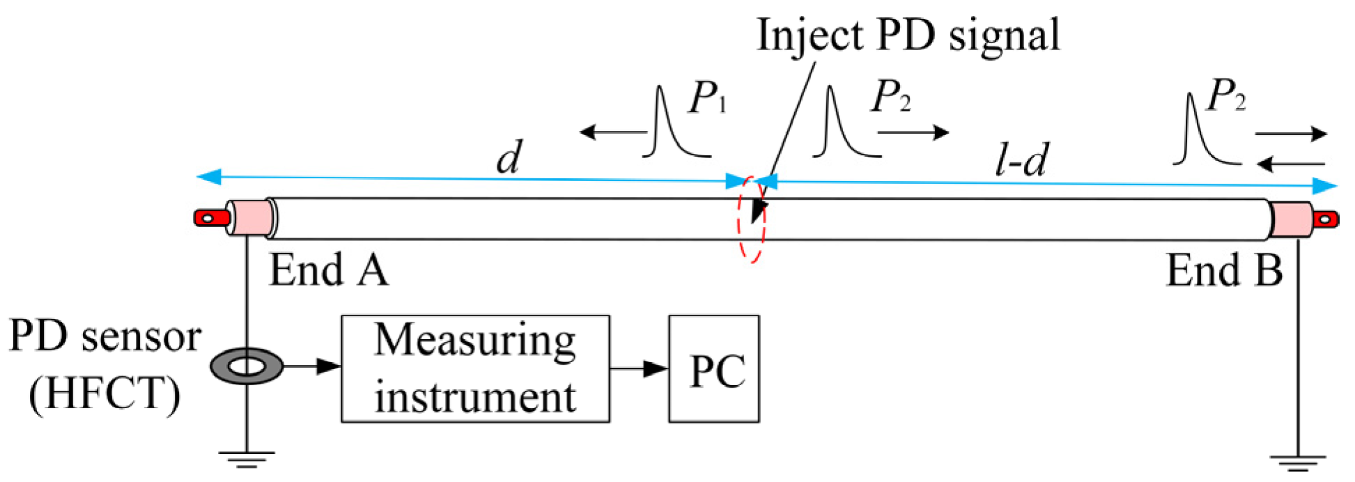
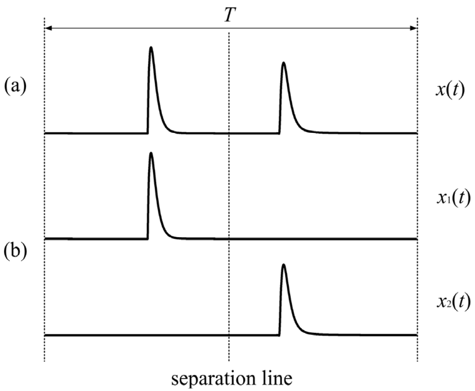
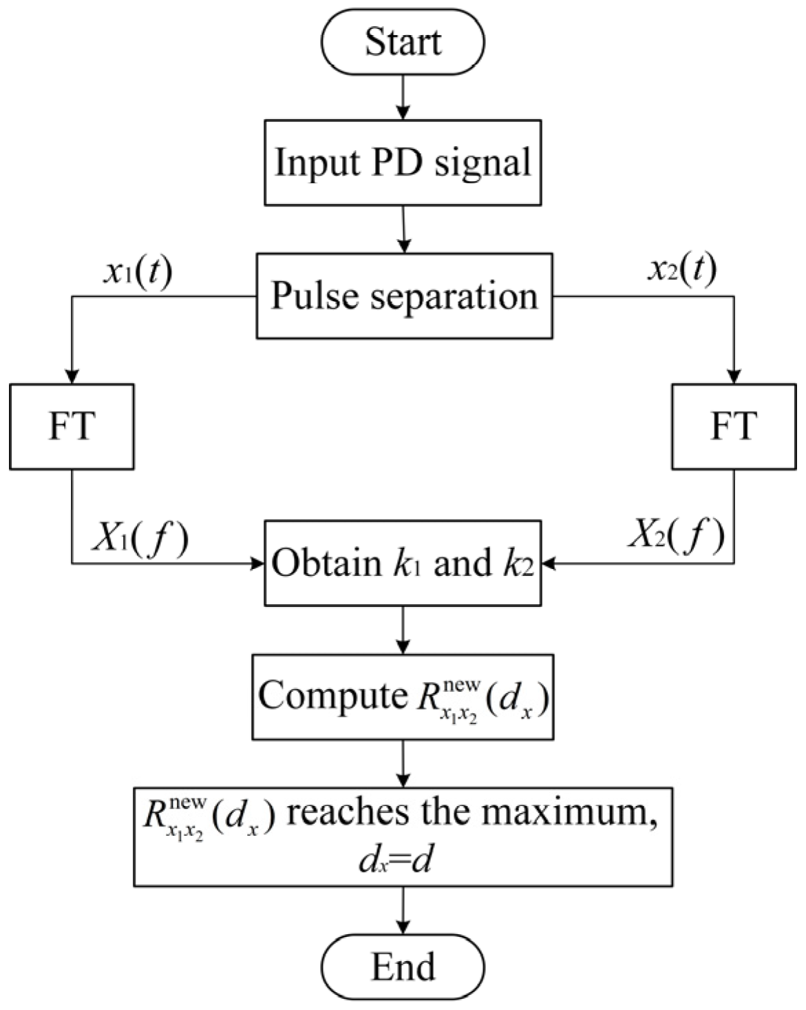
2. Principle of Cross-Correlation Method Based on Propagation Distance

Figure 1 illustrates a simplified single-ended PD measuring system, the length of the cable is l. The PD signal measuring instrument is connected to the test cable at end A. The remote end B is kept at open circuit. From Figure 1, the PD signal generated in the cable is simulated by injecting a narrow pulse at the distance of d from the end A. The injected PD signal will generate two pulses, and one pulse travels toward the measuring end A, and the other travels in the opposite direction toward the remote end B. Once one PD pulse reaches the remote end B, it is reflected and arrives later at the measuring end A, as illustrated in Figure 1. The first pulse is referred to as direct wave P₁, whereas the second pulse is reflected wave P₂.

In the proposed method, it is necessary to first obtain the direct wave and the reflected wave for the PD signals. According to the different arrival time at end A, the PD signal is divided into two windows by the separation line shown in Figure 2. The first window contains the direct wave denoted as x₁(t), whereas the second window contains the reflected wave denoted as x₂(t). From Figure 1, compared with the direct wave, the reflected wave has traveled an additional distance of 2(l − d).

Assuming a total record time length of T for each wave, then deriving the signals in the frequency domain using the Fourier transformation (FT) [15], we have the following:

$$X_1(f)={\displaystyle {\int }_0^T{x}_1}(t){\mathrm{e}}^{-\mathrm{j}2\mathsf{\pi }ft}\mathrm{d}t$$

(1)

$$X_2(f)={\displaystyle {\int }_0^T{x}_2}(t){\mathrm{e}}^{-\mathrm{j}2\mathsf{\pi }ft}\mathrm{d}t$$

(2)

where f is the frequency, and t is the time.

Because the PD pulse suffers from significant attenuation and dispersion as it travels in the cable, the reflected pulse X₂(f) is expressed as

$$X_2(f)=X_1(f){\mathrm{e}}^{-2\gamma (l-d)}=X_1(f){\mathrm{e}}^{-2\alpha (l-d)}{\mathrm{e}}^{-\mathrm{j}2\beta (l-d)}$$

(3)

where γ is the propagation constant, α is the attenuation constant, and β is the phase constant.

The new cross-correlation function of both signals is defined as

$$R_{x_1{x}_2}^{\mathrm{new}}(r)=\frac{1}{2\mathsf{\pi }}{\displaystyle {\int }_{-\infty }^{+\infty }{X}_1^{*}(f)}{X}_2(f){\mathrm{e}}^{\mathrm{j}\beta r}\mathrm{d}f$$

(4)

where r is the propagation distance, and * denotes the complex conjugate.

Replacing X₂(f) with Equation (3), we can obtain

$$R_{x_1{x}_2}^{\mathrm{new}}(r)=\frac{1}{2\mathsf{\pi }}{\displaystyle {\int }_{-\infty }^{+\infty }|X_1(f){|}^2{\mathrm{e}}^{-2\alpha (l-d)}}{\mathrm{e}}^{\mathrm{j}\beta (r-2l+2d)}\mathrm{d}f$$

(5)

The parameter d_x is defined as

$$d_x=l-r/2$$

(6)

Inserting Equation (6) into Equation (5), the cross-correlation function is expressed as

$$R_{x_1{x}_2}^{\mathrm{new}}(d_x)=\frac{1}{2\mathsf{\pi }}{\displaystyle {\int }_{-\infty }^{+\infty }|X_1(f){|}^2{\mathrm{e}}^{-2\alpha (l-d)}}{\mathrm{e}}^{\mathrm{j}2\beta (d-d_x)}\mathrm{d}f$$

(7)

When d_x = d, the function $R_{x_1{x}_2}^{\mathrm{new}}(d_x)$ reaches the maximum value, and the location of the PD source can be obtained.

The time domain waveform of field-detected PD signal is shown in Figure 3a. It was measured on a 10 kV XLPE cable system with a sampling rate of 200 MHz. Figure 3b shows the frequency domain waveform of field-detected PD signal. The PD signal only dominates the signal in the red area. The noise dominates the signal in most areas. Generally, as shown in Figure 3, the frequency band of the PD signal is narrow in actual tests [16]. Except for the center frequency, for the other frequency components, the PD amplitude spectrum is relatively low, and the noise dominates the signal. Thus, the new cross-correlation function can reduce the effects of noise by setting the upper and lower limits frequency in Equation (5). Meanwhile, both X₁(f) and X₂(f) are discrete signals, so Equation (5) should be rearranged as Equation (8).

$$R_{x_1{x}_2}^{\mathrm{new}}(d_x)=\frac{1}{k_2-k_1}{\displaystyle \sum _{k=k_1}^{k_2}{X}_1^{*}(k)X_2(k){\mathrm{e}}^{\mathrm{j}\beta (k)2(l-d_x)}},0<d_x<l$$

(8)

where k₁ and k₂ are the discrete points of upper and lower limits frequency, which is a band-pass filter [17].

Because the traditional positioning methods use the time delay between the direct wave and the reflected wave to locate the PD source, the positioning accuracy can be influenced by the sampling rate and frequency-dependent characteristic of phase velocity. As shown in Equation (8), because the proposed method uses the propagation distance instead of the time delay, it can eliminate the influences of the sampling rate and frequency-dependent characteristics of phase velocity on positioning accuracy.

Figure 4 contains a flowchart of the proposed PD location method. The direct wave x₁(t) and the reflected wave x₂(t) are obtained using the PD pulse separation procedure as described in Figure 2. The x₁(t) and x₂(t) are transformed into frequency domain signals using the FT. The output of this transformation is X₁(f) and X₂(f), respectively. The k₁ and k₂ are obtained by analyzing the frequency range of X₁(f) and X₂(f) to reduce the effects of noise. The function $R_{x_1{x}_2}^{\mathrm{new}}(d_x)$ is obtained using Equation (8), and it reaches the maximum value, the location of the PD source can be obtained.

3. Simulation Verification of the Positioning Method

To evaluate the performance of the proposed method, we simulated the PD cable pulse propagation through a computer. The cable model is a 10 kV XLPE cable with a length of l = 500 m, and

Table 1. The parameters of the simulated cable model [18,19].

Parameters	Value
radius of cable core rc (mm)	4
radius of shielding layer rs (mm)	9.5
resistivity of cable core ρc (μΩ mm)	17.5
resistivity of shielding layer ρs (μΩ mm)	17.5
conductivity of XLPE σ (S/m)	1 × 10−16
dielectric constant of XLPE ε (F/m)	2.04 × 10−11

shows the parameters. We injected the PD pulse at the distance of d = 250 m, which is in the middle of the cable. The distributed parameters of the cable can be approximately formulated as follows, according to [18,19]:

$$R\approx \frac{1}{2\mathsf{\pi }}\sqrt{\frac{{\mu }_0\omega }{2}}(\frac{1}{r_{\mathrm{c}}}\sqrt{{\rho }_{\mathrm{c}}}+\frac{1}{r_{\mathrm{s}}}\sqrt{{\rho }_{\mathrm{s}}})$$

(9)

$$L\approx \frac{{\mu }_0}{2\mathsf{\pi }}\ln \frac{r_{\mathrm{s}}}{r_{\mathrm{c}}}+\frac{1}{4\mathsf{\pi }}\sqrt{\frac{2{\mu }_0}{\omega }}(\frac{1}{r_{\mathrm{c}}}\sqrt{{\rho }_{\mathrm{c}}}+\frac{1}{r_{\mathrm{s}}}\sqrt{{\rho }_{\mathrm{s}}})$$

(10)

$$G=\frac{2\mathsf{\pi }\mathsf{\sigma }}{\ln (r_{\mathrm{s}}/r_{\mathrm{c}})}$$

(11)

$$C=\frac{2\mathsf{\pi }\mathsf{\epsilon }}{\ln (r_{\mathrm{s}}/r_{\mathrm{c}})}$$

(12)

where R, L, G, and C separately represent the unit resistance, inductance, conductance, and capacitance of the cable line in a distributed parameter model; r_c and r_s are the cable core and shielding layer radiuses, respectively; ρ_c and ρ_s are the resistivities of cable core and shielding layer, respectively; ${\mu }_0$ is the vacuum permeability, and ɛ is the dielectric constant of the XLPE material; σ is the conductivity of the XLPE material, whereas $\omega =2\mathsf{\pi }f$ is the angular frequency.

The PD cable propagation characteristic is simulated by using the transfer function s₁(t) [7], which is defined by the following:

$$s_1(t)=\mathrm{IFT}(S(\omega ){\mathrm{e}}^{-\gamma h})$$

(13)

where S(ω) is the FT of original PD signal s(t); IFT is the inverse Fourier transform; h is the propagation distance of s(t); and γ is defined by [19]

$$\gamma =\sqrt{(R+\mathrm{j}\omega L)(G+\mathrm{j}\omega C)}$$

(14)

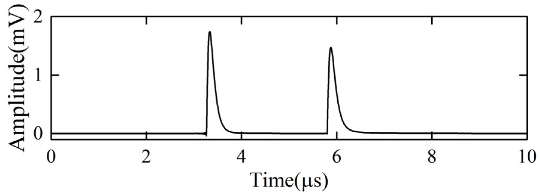
3.1. PD Signal Model

The PD signal is commonly represented by a double-exponential pulse [20,21], and it is given by

$$s(t)=A(e^{-1.3t/\tau }-e^{-2.2t/\tau })$$

(15)

where $\tau$ = 100 ns is the attenuation time constant of the PD signal, and the voltage multiplier A is 10 mV.

We injected the PD pulse at the distance of d = 250 m to obtain the PD waveform shown in Figure 5. The sampling rate is 100 MHz, and the time window T is 10 μs.

In the proposed method, the PD pulses must be split into the direct wave x₁(t) and the reflected wave x₂(t) using the pulse separation procedure, as illustrated in Figure 2. Figure 6 shows the magnitude-frequency spectrums of x₁(t) and x₂(t) using the FT.

Intuitively, with the increase in propagation distance, the signal becomes wider in the time domain (see Figure 5) and sharper in the frequency domain (see Figure 6). The frequency-dependent characteristic of phase velocity causes the differences of the waveform in the direct PD pulse and the reflected PD pulse, which will affect the accuracy of PD location through the traditional cross-correlation algorithm. The frequency range of the PD pulse is limited, as shown in Figure 6, so the method will obtain better noise resistance performance by setting proper parameters of k₁ and k₂, which are like a band-pass filter. k₁ and k₂ are set to 1 and 140 in Figure 6.

3.2. Results of the PD Location

Figure 7 displays the normalized CFD curve, and it reaches the maximum value when d_x = 250 m, so the proposed method can accurately locate the PD source. Meanwhile, Figure 7 shows the comparison of the normalized curves between the TCF and CFD. For the comparison, the independent TCF variable is converted from delay time to distance d_ς from the end A by Equation (16).

$$d_{\varsigma }=l-\overline{v}\varsigma /2$$

(16)

where ς is the delay time, and $\overline{v}$ is the mean of the high-frequency phase velocity.

Compared with TCF, because the CFD method considers the frequency-dependent characteristic of phase velocity in Equation (8), the CFD curve is more symmetrical and accurately locates the PD source. The value of parameter d_x in Equation (8) can be easily adjusted, but the value of parameter d_ς of the TCF curve is determined by the sampling rate, so the CFD curve has a higher resolution and is more smooth, which also makes the location accuracy higher.

Table 2. Comparison of location results.

Different Location Methods	Absolute Error (m)
PDM	1.57
ECA	0.41
TCF	0.58
CFD	0

shows the absolute error values of the PDM, ECA, TCF, and CFD at a distance of d = 250 m. The fixed phase velocity of PD pulses in PDM, ECA, and TCF is calculated by the mean of the high-frequency phase velocity. According to Table 2, the locating algorithm proposed in this paper has the smallest absolute error, thus obtaining higher positioning accuracy. The proposed method does not need to determine the point on the waves, which is important for the measurement of the arrival time interval. This is an advantage of the proposed algorithm over the traditional TOA evaluation methods, including PDM, ECA, and TCF.

3.3. The Influence of Propagation Distance on Localization Accuracy

With the increase in propagation distance, more distortion of the reflected wave would occur because of the attenuation and dispersion on the cable, which will affect the location accuracy. To analyze the effect of propagation distance on the location accuracy, we used different cable models with different lengths for comparison.

Similarly, we injected the PD pulse in the middle of the cables with different lengths to obtain absolute errors for the various PD location methods in Figure 8. The T is 50 μs.

For the traditional TOA evaluation methods, the location absolute error values will increase with the increase in propagation distance for the influences of phase velocity and waveform distortion. Compared with other algorithms, because the proposed locating algorithm considers the frequency-dependent characteristic of phase velocity, the method performs excellently and has minimal location error for the PD signal.

3.4. The Influence of the Sampling Rate on Localization Accuracy

The acquisition equipment sampling rate also affects the PD waveform. As a result, the location accuracy will be affected. To analyze the effects of the sampling rate on location accuracy, we changed the PD waveform sampling rate described in Section 3.1. Figure 9 shows the absolute errors of different sampling rates on the PD location estimation.

The equipment sampling rate will affect the location accuracy of traditional TOA evaluation methods. However, in all cases, the absolute error of the proposed locating algorithm approaches zero. When the sampling rate is low, the traditional TOA evaluation methods are difficult to accurately determinate the point on the waves. However, the proposed locating algorithm uses the propagation distance instead of the time delay. Even at a low sampling rate, it can also achieve a low positioning error.

In Figure 8 and Figure 9, we can obtain the accurate phase constant of cable in simulation, thus the CFD curve can accurately locate the PD source. On the other hand, the PD signal has no noise in Figure 8 and Figure 9. As a result, the absolute error of the proposed method approaches zero.

3.5. The Influence of White Noise on Localization Accuracy

The white Gaussian noise (WGN) is added into the simulated PD signal in Figure 5 to imitate the PD signal in actual conditions. Figure 10 shows the simulated PD pulse with three different signal-to-noise ratios (SNRs) white noises (i.e., 30 dB, 15 dB, and 5 dB). These SNRs represent small, moderate, and large noise, respectively.

To evaluate the localization effects of the four locating algorithms, the mean location error (MLE) is defined as [12]:

$$MLE=\frac{1}{p}{\displaystyle {\sum }_{i=1}^p\left|d_{\mathit{xi}}-d\right|}$$

(17)

where d_xi is the estimated location, and p = 100.

Table 3. Comparison of MLE values for different location methods at d = 250 m.

Different Location Methods	30 dB MLE (m)	15 dB MLE (m)	5 dB MLE (m)
PDM	1.26	1.90	11.83
ECA	0.41	0.79	23.11
TCF	0.58	0.89	2.50
CFD	0.06	0.36	1.34

shows the results of the MLE of the four location methods at a distance of d = 250 m. In the noisy environment with an SNR of 30 dB to 5 dB, the location algorithm proposed in this paper has the lowest MLE values, thus obtaining higher positioning accuracy. Figure 11 shows the statistical analysis of different location methods under 15 dB. Compared with the four location methods, the location algorithm proposed in this paper has the smallest diversity of results, and the max location absolute error is less than 0.5%. It should be noted that k₁ and k₂ in Equation (8) are set to 1 and 50, respectively, to reduce the influences of WGN.

4. Experimental Verification of the Method

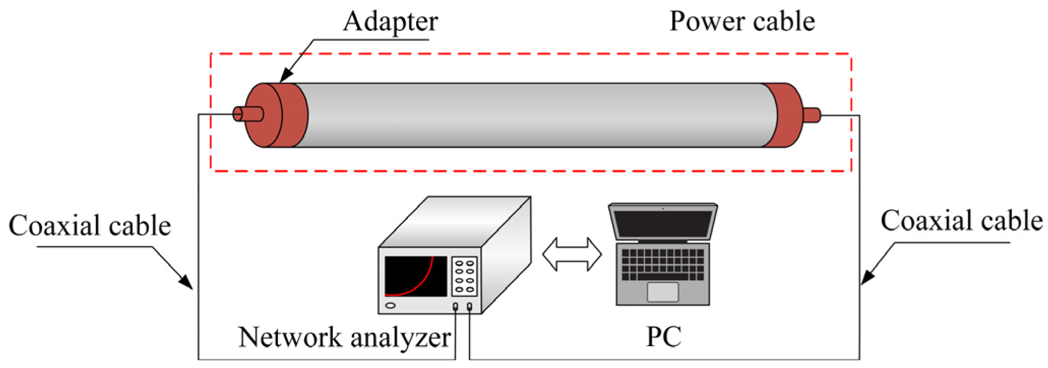
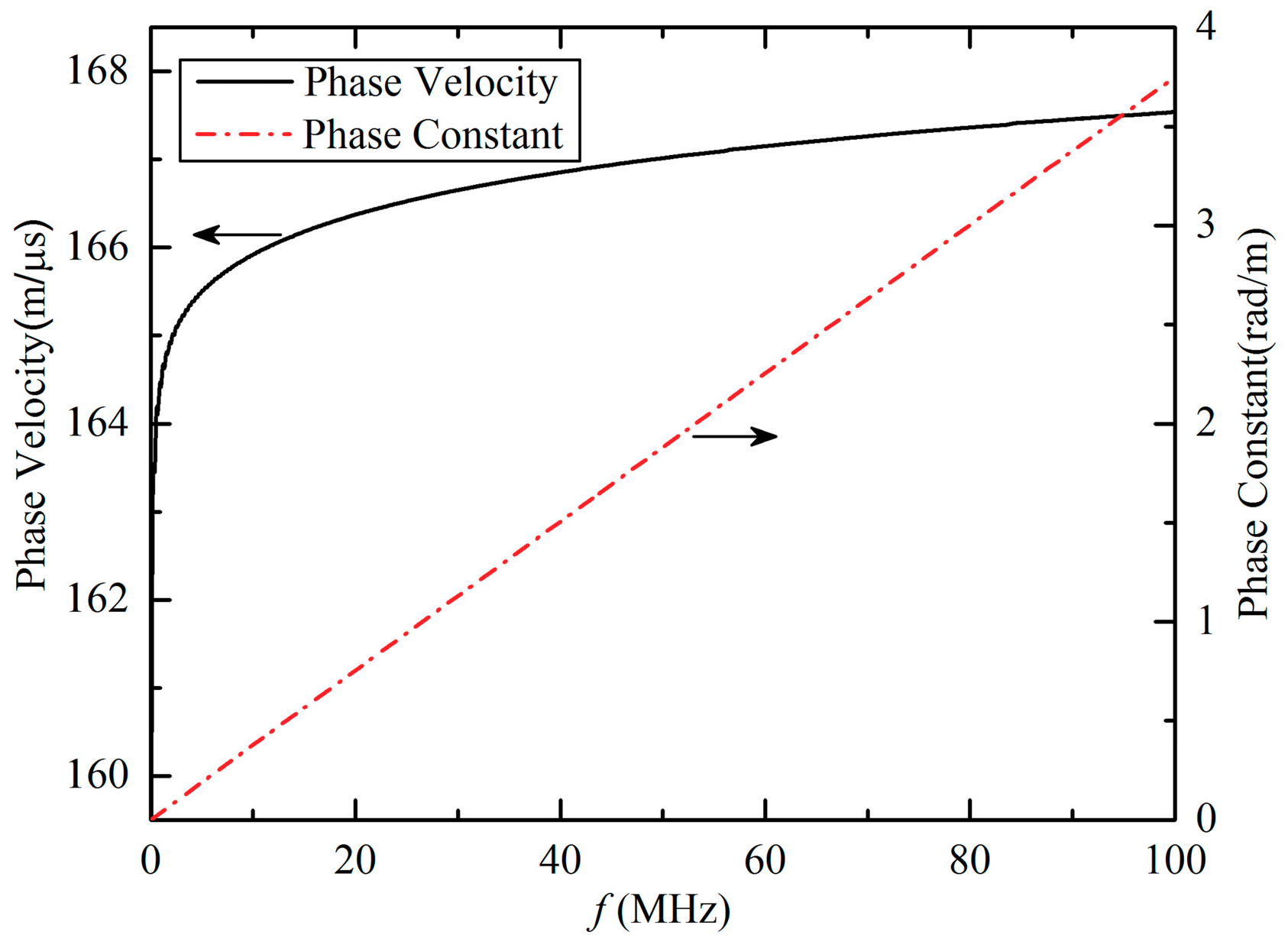
4.1. Measurement of the Phase Constant

In the proposed method, the cable phase constant should be obtained before locating the PD source. Figure 12 shows a simplified phase constant measuring system. Because a cable is considered to be a two-port network, we can realize the accurate measurement of the phase constant by using the s-parameter (i.e., the scattering parameter) measured by a vector network analyzer. The s-parameter is a networking parameter established on the relationship between the incident and reflected waves, which is applicable to a distributed parameter circuit cable model. When inputting a sweep signal on the test cable, we can measure the s₂₁-parameter to obtain the phase constant of the cable [18].

Figure 13 provides the measured phase constant and phase velocity of the 10 kV XLPE power cable. From Figure 13, the results indicate that the phase velocity changes with signal frequency, which should be considered in PD localization.

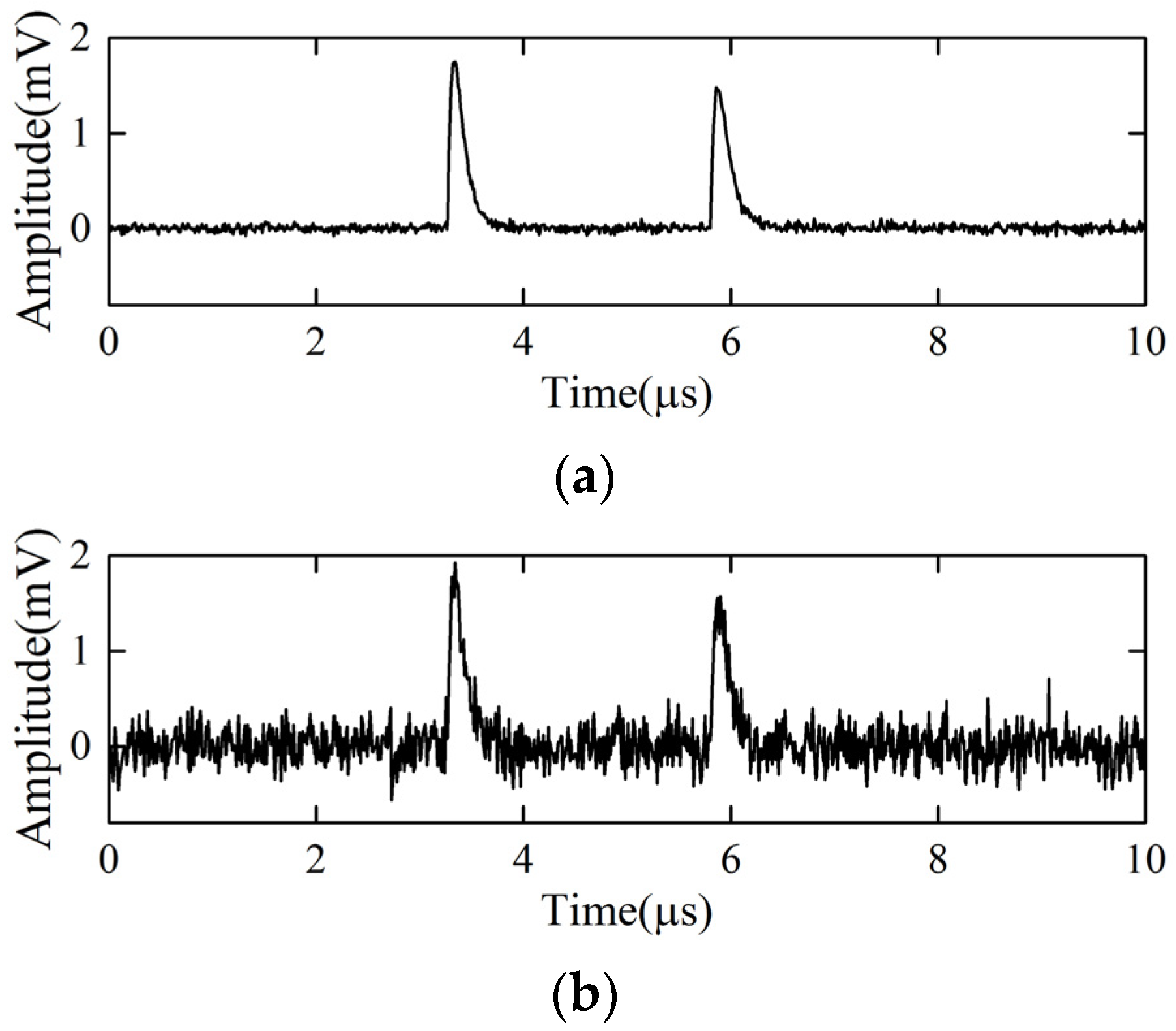
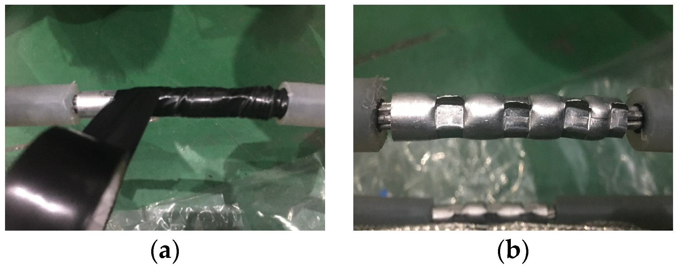
4.2. Location Experiment of the PD Source

We used a damped oscillation wave testing system with HFCT [22] to obtain PD signals for location. By taking two 10 kV defective XLPE cables for the test, we performed PD locations based on different location methods for the cables. Figure 14 illustrates the defects. Defect 1 is that the insulating tapes are used as the semi-conductive tapes on the conductor in a joint by mistake, and defect 2 is that the metal tips are not polished in the joint.

Both the defects are at the distance of d = 100.5 m from the end A, and both the lengths of two defective cables are 250 m. The applied DC voltage is 22 kV, and the sampling rate is 200 MHz. Figure 15 shows the captured PD waveforms.

The four location methods are used to process the PD signals shown in Figure 15, and

Table 4. Comparison of absolute error values for the different location methods in measured PD signals.

Different Location Methods	Defect 1		Defect 2
	Estimated Location (m)	Absolute Error (m)	Estimated Location (m)	Absolute Error (m)
PDM	99.28	1.22	97.19	3.31
ECA	98.44	2.06	97.61	2.89
TCF	98.44	2.06	97.61	2.89
CFD	100.75	0.25	100.80	0.30

displays the different results. According to the results in Table 4, the locating algorithm proposed has the lowest absolute error, thus having higher positioning accuracy.

5. Conclusions

In this paper, we present a new method for locating a power cable PD source. The proposed method uses the cross-correlation function based on the propagation distance of the PD pulse. The PD source location can be determined when the value of the cross-correlation function reaches the maximum value. This method does not need to estimate arrival time. As a result, the problem of the estimation error of arrival time interval and the frequency-dependent characteristic of phase velocity can be avoided in the traditional TOA evaluation methods.

We evaluated the performance of the proposed method quantitatively through the simulations. The statistical results demonstrate that the proposed method can greatly reduce the effect of propagation distance, sampling rate, and white noise on PD localization accuracy. Further experimental results indicate that the locating algorithm can accurately locate the PD source in power cables.

References

1. Eigner, A.; Rethmeier, K. An overview on the current status of partial discharge measurements on AC high voltage cable accessories. IEEE Electr. Insul. Mag. 2016, 32, 48–55. [Google Scholar] [CrossRef]
2. Shafiq, M.; Kiitam, I.; Kauhaniemi, K.; Taklaja, P.; Kütt, L.; Palu, I. Performance comparison of PD data acquisition techniques for condition monitoring of medium voltage cables. Energies 2020, 13, 4272. [Google Scholar] [CrossRef]
3. Mohamed, F.B.; Siew, W.H.; Soraghan, J.J.; Strachan, S.M.; McWilliam, J. Partial discharge location in power cables using a double ended method based on time triggering with GPS. IEEE Trans. Dielectr. Electr. Insul. 2013, 20, 2212–2221. [Google Scholar] [CrossRef]
4. Shafiq, M.; Kauhaniemi, K.; Robles, G.; Isa, M.; Kumpulainen, L. Online condition monitoring of MV cable feeders using Rogowski coil sensors for PD measurements. Electr. Power Syst. Res. 2019, 167, 150–162. [Google Scholar] [CrossRef]
5. Mahdipour, M.; Akbari, A.; Werle, P.; Borsi, H. Partial discharge localization on power cables using on-line transfer function. IEEE Trans. Power Deliv. 2019, 34, 1490–1498. [Google Scholar]
6. Cavallini, A.; Montanari, G.C.; Puletti, F. A novel method to locate PD in polymeric cable systems based on amplitude-frequency (AF) map. IEEE Trans. Dielectr. Electr. Insul. 2007, 14, 726–734. [Google Scholar] [CrossRef]
7. Sheng, B.; Zhou, C.; Hepburn, D.; Dong, X.; Peers, G.; Zhou, W.; Tang, Z. A novel on-line cable PD localisation method based on cable transfer function and detected PD pulse rise-time. IEEE Trans. Dielectr. Electr. Insul. 2015, 22, 2087–2096. [Google Scholar] [CrossRef] [Green Version]
8. Zhang, Z.S.; Xiao, D.M.; Li, Y. Rogowski air coil sensor technique for on-line partial discharge measurement of power cables. IET Sci. Meas. Technol. 2009, 3, 187–196. [Google Scholar] [CrossRef]
9. Kreuger, F.H.; Wezelenburg, M.G.; Wiemer, A.G.; Sonneveld, W.A. Partial discharge. XVIII. Errors in the location of partial discharges in high voltage solid dielectric cables. IEEE Electr. Insul. Mag. 1993, 9, 15–22. [Google Scholar] [CrossRef]
10. Wagenaars, P.; Wouters, P.A.A.F.; Wielen, P.C.J.M.; Steennis, E.F. Accurate estimation of the time-of-arrival of partial discharge pulses in cable systems in service. IEEE Trans. Dielectr. Electr. Insul. 2008, 15, 1190–1199. [Google Scholar] [CrossRef]
11. Markalous, S. Detection and Location of Partial Discharges in Power Transformers Using Acoustic and Electromagnetic Signals. Ph.D. Thesis, Universitaet Stuttgart, Stuttgart, Germany, 2006. [Google Scholar]
12. Lan, S.; Hu, Y.; Kuo, C. Partial discharge location of power cables based on an improved phase difference method. IEEE Trans. Dielectr. Electr. Insul. 2019, 26, 1612–1619. [Google Scholar] [CrossRef]
13. Mardiana, R.; Su, C.Q. Partial discharge location in power cables using a phase difference method. IEEE Trans. Dielectr. Electr. Insul. 2010, 17, 1738–1746. [Google Scholar] [CrossRef]
14. Hou, H.; Sheng, G.; Jiang, X. Robust time delay estimation method for locating UHF signals of partial discharge in substation. IEEE Trans. Power Deliv. 2013, 28, 1960–1968. [Google Scholar]
15. Piersol, A. Time delay estimation using phase data. IEEE Trans. Acoust. Speech. Signal Process. 1981, 29, 471–477. [Google Scholar] [CrossRef]
16. Jin, T.; Li, Q.; Mohamed, M.A. A novel adaptive EEMD method for switchgear partial discharge signal denoising. IEEE Access 2019, 7, 58139–58147. [Google Scholar] [CrossRef]
17. Ichige, K.; Iwaki, M.; Ishii, R. Accurate estimation of minimum filter length for optimum FIR digital filters. IEEE T Circuits-II 2000, 47, 1008–1016. [Google Scholar] [CrossRef]
18. Zhang, A.; Gao, C.; Yang, W.; Zhou, Z.; Li, Q. Propagation coefficient spectrum based locating method for cable insulation degradation. IET Sci. Meas. Technol. 2019, 13, 363–369. [Google Scholar] [CrossRef]
19. Zhou, Z.; Zhang, D.; He, J.; Li, M. Local degradation diagnosis for cable insulation based on broadband impedance spectroscopy. IEEE Trans. Dielectr. Electr. Insul. 2015, 22, 2097–2107. [Google Scholar] [CrossRef]
20. Zhou, K.; Li, M.; Li, Y.; Xie, M.; Huang, Y. An improved denoising method for partial discharge signals contaminated by white noise based on adaptive short-time singular value decomposition. Energies 2019, 12, 3465. [Google Scholar] [CrossRef] [Green Version]
21. Ghorat, M.; Gharehpetian, G.B.; Latifi, H.M.; Hejazi, A. A new partial discharge signal denoising algorithm based on adaptive dual-tree complex wavelet transform. IEEE Trans. Instrum. Meas. 2018, 67, 2262–2272. [Google Scholar] [CrossRef]
22. Zhu, G.; Zhou, K.; Zhao, S.; Li, Y.; Lu, L. A novel oscillation wave test system for partial discharge detection in XLPE cable lines. IEEE Trans. Power Deliv. 2020, 35, 1678–1684. [Google Scholar] [CrossRef]
Figure 1. Block diagram of the single-ended PD measuring system.
Energies 13 04549 g001
Figure 2. The PD pulses; (a) before pulse separation; (b) after pulse separation.
Energies 13 04549 g002
Figure 3. Time domain and frequency domain waveforms of the PD signal in a practical test. (a) Time domain waveform; (b) Frequency domain waveform.
Energies 13 04549 g003
Figure 4. Block diagram of the proposed PD location algorithm based on distance.
Energies 13 04549 g004
Figure 5. The time domain waveform of the simulated PD pulse for the defect at d = 250 m.
Energies 13 04549 g005
Figure 6. The frequency domain waveform of simulated PD pulse for the defect at d = 250 m.
Energies 13 04549 g006
Figure 7. The normalized curves of the TCF and CFD.
Energies 13 04549 g007
Figure 8. The absolute error values for various location methods of the cables with different lengths.
Energies 13 04549 g008
Figure 9. The absolute error values for various sampling rates of the PD pulse waveform.
Energies 13 04549 g009
Figure 10. The time domain waveforms of the simulated PD pulse with different SNRs. (a) 30 dB; (b) 15 dB; (c) 5 dB.
Energies 13 04549 g010
Figure 11. Statistical analysis of different location methods under SNRs = 15 dB.
Energies 13 04549 g011
Figure 12. Schematic diagram of the phase constant measuring system.
Energies 13 04549 g012
Figure 13. Phase constant and phase velocity of the 10 kV XLPE power cable.
Energies 13 04549 g013
Figure 14. Schematic diagram of cable defects. (a) The insulating tapes are used as semi-conductive tapes by mistake; (b) The metal tips are not polished.
Energies 13 04549 g014
Figure 15. Measured PD waveforms of defective cables. (a) The electrical tapes are used for the semi-conductive tapes by mistake; (b) The metal tips are not polished.
Energies 13 04549 g015