Abstract
The feasibility of electricity production via solar energy in the Middle East is high due to the enormous value of solar radiation. Building-integrated photovoltaics (BIPV) are systems used to utilise the unused spaces that can be installed on the façade or roof by replacing the building’s main element. However, the main problem associated with electricity production by BIPV is partial shading on the roof, which can produce multiple hot spots and disturbances to the system if the insolation values within the whole BIPV array vary. Partial shading, in this case, is observed due to the complexly shaped roof. This paper studies the partial shading effect on one of Qatar’s most recent projects (metro stations), and models the Education City station, which is a major station. The rooftop is complex, and it has many wavy shapes that can affect the BIPV system’s performance. The station is modelled using building-information modelling (BIM) software, wherein all of the station’s models are gathered and linked using BIM software to illustrate the BIPV and indicate the solar insolation distribution on the rooftop by simulating the station’s rooftop. The system is optimised for maximum yield to determine the optimal configuration and number of modules for each string using a genetic algorithm. The outcomes from the algorithm are based on clustering the solar insolation values and then applying a genetic algorithm optimisation to indicate the optimum BIPV array layout for maximum yield.
1. Introduction
There has been major growth and improvement in utilising solar energy worldwide, as it is considered one of the most reliable and significant renewable and green energy sources. A remarkable quantity of research has been conducted to develop the quality and efficiency of the energy generated by Photovoltaics (PVs) [1]. Recently, world energy consumption has been 10 TW and this is expected to reach 30 TW by 2050; however, the additional 20 TW needs to be generated with renewable energy with zero CO2 emissions in order to stabilise the CO2 levels in our atmosphere [2]. Therefore, much work is in progress to implement PV systems in major building projects, which can result in less CO2 associated with these projects and more free electricity generation for use within the buildings. These efforts can decrease greenhouse gas emissions and create economic savings [2,3]. Qatar is planning to create a megaproject targeted to produce 2%, or 200 MW, of the nation’s electricity via PVs by 2020 and 20%, or 2 GW, of the nation’s electricity via PVs by 2030. The country’s CO2 emissions will be remarkably decreased, as 0.24 million tonnes of oil equivalent (Mtoe) and 2.13 Mtoe will be saved from natural gas by 2020 and 2030, respectively, which will reduce the CO2 emissions in Qatar by 0.51 Mt and 4.5 Mt by 2020 and 2030, respectively [4].
Qatar can be classified as having a high intensity of solar irradiance, which aids in high energy productivity of any PV system installed in the country. These systems can generate electricity easily all over the country due to the high intensity of solar irradiance [5,6]. However, the environment in Qatar is considered harsh, and the temperature, dust, and humidity are key factors in the generation productivity of PV systems, and these conditions can cause PV performance to degrade. Therefore, it is recommended to choose the most suitable PV module technology with respect to Qatar’s environment [7].
To achieve the goals of a sustainable environment, saving major resources, achieving Qatar’s vision 2030, and hosting a carbon-neutral 2022 FIFA world cup, the availability and the adoption of PV plants around Qatar and installing PV systems in Qatar major projects, such as metro stations and the world cup stadium, will greatly help in achieving them [8,9]. Consequently, Building-integrated photovoltaics (BIPV) can be installed in many of the major projects, as they do not need huge spaces and the rooftops and façades of these major projects can be utilised effectively by placing BIPV modules on them in order to generate clean electricity and to offset the high CO2 rates that caused by the building sector globally [10]. However, doing so will also be challenging due to the environmental conditions in Qatar. Transparent BIPV modules are largely replacing the glass in building façades, and thin-film modules can be fitted on rooftops [11]. It has been shown that, if a building has its glass replaced with transparent BIPV, this generates 40% of the buildings’ energy needs. Moreover, BIPV are considered aesthetically better than normal roof-mounted PVs [12,13].
An experimental study by Touati et al. indicated that amorphous silicon PV performed the best in Qatar’s harsh environment compared to other PV modules such as mono-crystalline, and it showed better stability in energy production and degradation [14,15]. Moreover, the main contribution of their article is the optimisation technique, which can be applied to any PV cell technology based on the study and any environmental conditions.
This paper will discuss the feasibility of applying the concept of building-information modelling with an optimisation algorithm. Al-Janahi et al. (2019) analysed the partial shading on geometrically complex roofs and the process of mitigating the partial shading issue. However, it analysed one section of a model and used a manual optimal configuration to mitigate the partial shading [16]. In this paper, the whole area of the model will be considered for partial shading analysis and solar insolation simulation. In addition, genetic algorithm optimisation method will be adopted to optimally configure the BIPV array in the model, predict the optimal energy extraction, and model an energy analysis for the station.
1.1. Partial Shade Condition in BIPV Array
Generally, different types of energy loss can be associated with any BIPV system. There can be losses due to electrical connections, high temperatures, orientation, tile, and shade. These losses will lead to less than optimal power output if they are not studied. Shade should be considered during the design phase of any BIPV system because there are different insolation values directed toward different parts of the same BIPV array, which will result in different current-voltage (I-V) values within the system. This difference will disturb the system and limit its energy output to its lowest I-V value. In addition, shade can reduce the energy output of the whole system’s peak power by 25%. To achieve the optimum energy output, all parameters, including inverters, module connections, and electrical simulations, should be designed to optimise the necessary output [17,18]. Shade is the main problem for many BIPV applications and can be caused by the environment, objects, or the shape of roofs. Shade on BIPV modules leads to electrical mismatch and overheating of the modules, which can cause multiple peak values of an I-V curve due to the different insolation values on the same array modules [19,20]. Zomer et al. (2016) discussed the performance of a 75-kWp BIPV system installed in a high-rise commercial building in Singapore. It contained multiple PV strings connected by multiple subsystems. Their shade analysis showed that the total shade percentage reached up to 12.8%. The main reasons for this partial shade on this BIPV system was due to neighbouring buildings or the position of the shading sensor. This sensor measures the shading percentage in a specific location, and sometimes the location of the sensor causes inaccurate measurements. Moreover, the sensor in the study measured the irradiance to be between 1110 and 1360 kWh/kWp and the Performance Ratio (PR) ranged from 80% to 90% of the system maximum yield because of the partial shading of the system [20]. Similarly, Gallardo-Saavedra and Karlsson (2018) investigated shade on a BIPV system under different circumstances. In a first test, seven cases were analysed in terms of the number of modules. and 37% shade was found in the modules for each case. In Case 1, even though one module was shaded by 37%, the output current was the same as the standard condition where no modules were shaded. This was mainly due to the bypass diode, which measured the difference in current. In the remaining five cases (2–6), there were 2–5 modules shaded in a row for each module with 37% shade, and the current output was limited by the shaded modules to 3.6 A and the bypass diode did not work. At the end, if two to five modules were shaded with the same shade percentage in the same row, the same current would be output for the system. In a second test, one to three cells in the modules were shaded with different percentages in seven cases again. If one to three cells were shaded with different shade percentages, the power output would be nearly the same but with 35% less power output than in the standard condition [21].
1.2. Building-Information Modelling (BIM) and Solar Irradiance Analysis
Building-information modelling (BIM) can be utilised to predict the insolation values for every day throughout the year for any object, as it can predict the performance of any building and the energy it needs [22]. In addition, it can digitally represent the physical building and the facility’s characteristics; furthermore, the BIM platform can be the basis for data sharing for all stakeholders. BIM is considered a sophisticated tool for accurately measuring irradiance data throughout the year. Many studies used BIM to gain the irradiance data needed for modelling buildings. The design of the BIPV should be considered during the design phase, as the architectural design of the building will affect the radiation of the installed BIPV system, which will then affect the electricity generated by the BIPV system and the electrical connection related to the system [23,24]. It is recommended that BIPV information be integrated into the BIM database to develop the constructability of the BIPV during the design stage. In addition, BIM is a friendly tool for technically evaluating a BIPV system and for doing solar insolation analysis [25,26].
However, BIM software can also be used to measure the insolation values for certain periods and areas at any time during the year. A case study used BIM to predict the PV power output of a 2.5-kWp PV system installed in Cardiff. The results showed that there was an average error of 4.2% between the monitored and simulated results [24]. Dixit and Yan (2012) used BIM to obtain solar insolation data for three different cities: Jacksonville, Florida; Dallas, Texas; and Brunswick, Georgia. Their results showed that, by using BIM, specifically Autodesk Revit (Autodesk, San Rafael, CA, USA), the insolation values of the simulated and measured insolation values were nearly the same within ±10% of the measured values [27]. In the same field, Gui et al. (2017) modelled the irradiation of a building. Their results showed that some modules have low irradiation values; thus, it was possible to optimise the system by reducing the number of modules which can be neglected due the low irradiance values received by them using Autodesk Revit [23]. Furthermore, BIM energy-based BIPV analysis was carried out by Kuo et al. (2016) to validate the measured real data with simulated data using BIM software (Autodesk Revit). The information for the analysis was validated, such as the location, weather data, orientation, longitude, and latitude of the model in real life. The results showed that the simulated results were approximately accurate compared to the measured values used at the building because, at the building site, the measured irradiance was obtained using pyranometers and then compared with the irradiance simulated by BIM. This caused a small error between the electricity outcomes, but it can be assumed that the results were approximately the same [28].
1.3. Optimising BIPV System Layout Using a Genetic Algorithm (GA)
Energy maximisation should be done by finding the most optimal configuration of a BIPV system. If the tilt and orientation change, the energy outcome will change due to the different direction of irradiation due to partial shade, which will enable the determination of the optimal layout configuration of any BIPV system under different partial shade conditions. A designed BIPV system based on the orientation of the sun for which the energy output will be optimised and how the BIPV modules are placed. However, the authors did not rely on any optimisation algorithms to increase the energy output [29]. There are many techniques that can be used to optimise the BIPV system by determining the most applicable configuration of the BIPV strings.
Krishna and Moger (2019) discussed several optimisation techniques and algorithms to reconfigure the system to mitigate the partial shade effect on PV systems. First, in the uniform irradiance condition, the PV modules’ system received the same irradiance value throughout the modules, which guaranteed that the system had the same maximum power and that there was only one peak value in I-V and power voltage (P-V) of the BIPV system. However, this is not the case for the partial shading condition. With the partial shading condition, some of the modules were shaded, thus receiving less irradiance than the unshaded modules. This may cause hot spots in the system and damage to the PV’s cells and modules. Therefore, there will be mismatch losses throughout the system, which can be caused by different temperatures and irradiance values. Furthermore, with the partial shading condition, the maximum power was less than that achieved under the uniform irradiance conditions. These losses cannot be totally prevented but can be mitigated using several methods.
One of the most used techniques is using a bypass diode for each module, which provides the path for the current, which it will allow or prevent based on the current generated by the modules, which depends on the solar irradiance and the elimination of the hot-spot problem in the system. Adding bypass diodes is classified as a passive technique to mitigate the partial shading condition of a BIPV system. However, active techniques are more effective, including reconfiguration strategies, which are classified as the most promising techniques for this category for minimising the partial shade effect. Reconfiguration techniques are based on irradiance levels and work by interconnecting the modules with each other as needed to reduce the mismatch losses and maximise the power output.
There are two main reconfiguration techniques: Total Cross-Tied (TCT) and Series-Parallel (SP). For TCT, all the modules with the same irradiance level are connected in one row to equalise the irradiance level. The SP technique is used to connect all the modules with the same irradiance level in a series in one string and then connect all the strings in parallel. As a result, the output current is not limited to the lowest irradiance-exposed module in the string.
The most commonly used algorithm for adopting any static or dynamic reconfiguration is a Genetic Algorithm (GA). It has been used to identify the most optimum reconfiguration that arranges switches under partial shading such that the current in each row is the optimum and to connect the modules with the same irradiance level in one string [30,31]. A GA is used to solve optimisation problems by using the algorithms to generate the next generation by selecting two individuals, which are considered parents [32,33]. These algorithms are based on techniques from evolutionary biology like mutation, selection, and crossover. To begin, random individuals need to be generated to create an initial population. Typically, the initial population can have hundreds or thousands of solutions. The next step is to select a portion of the initial population to breed a new generation. The solutions with higher fitness values are selected and the solutions with lower fitness values are discarded. The next step is crossover, where parents are selected from the fitness pool generation to generate a new child. This new child will have many characteristics from the parents. The next step is mutation, which ensures that the individuals are different. The mutation step is important for maintaining the genetic diversity of the population and achieving the desired global optimum [34,35].
Ismail et al. (2013) used a GA to extract the most optimal parameters of simulated solar panels. The GA analysed different cases to predict the optimum parameters for the solar panels and then these parameters were used as optimum ones throughout the simulation [33]. Deshkar et al. (2015) discussed the different reconfiguration of 9 × 9 PV modules in three cases with different partial shade distributions. A GA was used to reveal the best power output from the PV array [32]. The same approach was discussed by Rajan et al. (2017) concerning a 9 × 9 PV array with different distributions of shade. The method changed the electrical connection so that each row had the same irradiance level while keeping the physical locations of the modules the same. Their results showed good performance, and power generation was improved by 44.14% when a GA was used [36].
1.4. Novel Approach
In this paper, we implement the novel approach of linking BIM to GA. Qatar has a high intention toward solar irradiance, and the country is now looking to reduce its CO2 footprint. Consequently, a case study on the Qatar Rail metro station will be analysed. The choice of the Qatar Rail metro station was made because it is a new major infrastructure project in Qatar used by the public. In addition, the rooftop of the station is curved, which will help us analyse changes in the irradiance level of the BIPV system. The general method for the paper is as follows. Firstly, the BIM model of the station is created. Secondly, a BIPV array on the rooftop of the station is integrated in the BIM model. Thirdly, a solar analysis is simulated to determine the irradiance level at each module. Finally, the system is optimised to overcome the multiple peaks and to eliminate the hot spot of the system by levelling up the irradiance level for each string using a GA. The sequence of modelling this approach is shown in Figure 3. The papers reviewed used either only BIM, such as [37] and [28], or they only used GA optimisation techniques on random solar irradiance values, such as [36] and [32]. Therefore, the novelty of the paper is that it uses the model of the station, then simulates the solar irradiance data of the station model using BIM, and then determines the best configuration of the BIPV system using a GA optimisation method that optimises based on real simulated values.
2. Case Study
Qatar is currently developing a new major infrastructure project related to the transportation sector in the country, and this paper’s methodology is applied to this real case. Qatar built a new metro network, which has 37 stations across its three main lines. Some of these stations are elevated and others are underground. However, the underground stations have their main entrances at ground level. These main entrances’ shelters have no purpose except to provide accesses to the station. Therefore, installing BIPV on these shelters will reduce the energy demand on the grid, which is a good utilisation of the free areas on their roofs. In addition, this study will satisfy the implementation of optimisation method under partial shading for BIPV modules and mitigate the effect of partial shade. The roofs of Doha Metro entrances are complexly shaped, making them a good example for analysing the effect of partial shading. Moreover, to examine the weather conditions in a practical example, as Qatar has high solar insolation values across the year, with an average of 4449 h of sunlight per year, which entails that there is sunlight for 70% of the year [5]. However, the environment of Qatar is harsh and the high temperature, high moisture, and dust affect the performance of the PV [15]. The chosen station shelter is at the Education City station. This station was chosen because it is considered one of the two major stations across the whole network; thus, it is a good example for helping the public realise the importance of clean energy [38,39]. The building of this station started in 2013 and finished by early 2019. The station began operating by the end of 2019. Its architecture draws inspiration from the arch expressions of Islamic architecture, the lightness of the dhow sail, and the tensile profiles of the nomadic tents. The “vaulted spaces” design signals a step forward in the interpretation and morphological implementation of these elements. In other words, these elements represent the values of the country and are reflected in the sophisticated curvatures of the roof. Figure 1 shows the rooftop curvature of the Education City metro station with the dimensions of the roof and the height of the station. Figure 2 shows the perspective view of the station.
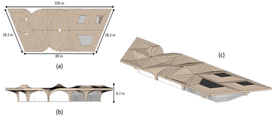
Figure 1.
Building-information modelling (BIM) model of the Education City metro station in different orientations. (a) Top view with the roof’s dimensions, (b) front view with height, (c) 3d view.
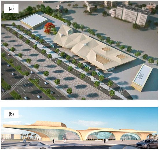
Figure 2.
Perspective view of the Education City station shelter. (a) Top view (b) side view.
Amorphous Silicon (a-Si) showed the best performance in Qatar’s weather [14,15]. Therefore, an integrated a-Si PV was chosen for analysing the energy performance of the system in this application. Table 1 describes the electrical characteristics of the a-Si module chosen for the case study, which is a 146-W module factory-made by Xunlight. After searching PV databases, including the System Advisor Model (SAM) and web database, this module was chosen because it is an a-Si module and it can be integrated with a building as a BIPV. The technology of this module is thin-film a-Si, and it can be used with BIPV. The electrical characteristics and data sheet for this module can be extracted from SAM and web databases [40,41].

Table 1.
Data sheet/electrical characteristics of the selected module Xunlight XRS18-146 [40,41].
3. Methods
The method primarily consists of modelling the whole system using several equations of the PV cell, module, and array. The equations will represent the interconnections between the several parameters that can affect the current, voltage, and power output, which will help model the PV system. The next step will concentrate on gathering the insolation data, which was achieved using BIM software (Revit), to assess the difference in insolation values across the rooftop of the Education City station in the Doha Metro network. Then, the best electrical connection for the modules installed on the rooftop of the station entrance are identified using GAs in Matlab/Simulink. A GA is used to optimise the BIPV system to maximise power generation, which mostly depends on the insolation absorbed by the modules.
3.1. BIPV Modelling Using Equations
The PV cell performs the key role of converting sunlight directed toward the cell, which contains photons that can free the electrons inside the cell. Electricity is produced by the motion of electrons within the cell. Nevertheless, the solar irradiance, ambient and cell temperatures, and operating voltage can create huge differences in the system’s current and voltage and, thus, power. Generally, PV cells, modules, and arrays show nonlinear I-V and P-V curve characteristics. Solar insolation and temperature play key roles in these characteristics, which can affect the current and voltage limits for the whole system. However, to examine the performance and behaviour of the PV cell, module, and array, we need to model the whole system under different insolation values in the case of partial shade to determine the I-V and P-V characteristics of the system. Several equations pointed in the Appendix A are used to represent the cell and module and array models to determine the relationships between the parameters and the effect of insolation [42,43].
PV Modules/Arrays Modelling
In this paper, we focus more on modelling whole PV modules and arrays than determining the effects on single cells, as partial shade affects the performance of the modules and arrays in general rather than single cells. Moreover, partial shade is considered according to the effect on the modules and arrays. Usually, the cells are connected in a parallel series form of PV modules. PV modules are connected in a parallel series to reach the optimum power requirements of the PV array. PV arrays are groups of PV modules that are connected to provide the required power output. The PV modules and arrays can be modelled to determine the power from current (I) and voltage (V) using the following equations [44]:
IPH is the photocurrent (A), IS is the saturation current (A), q is the electron charge (=1.6 × 10⁻¹⁹ °C), k is Boltzmann’s constant (=1.38 × 10⁻²³ J/K), and TC is the cell’s operating temperature (K). The reference operating cell temperature is 298 K (25 °C). A is the ideal factor, which depends on the technology the cell uses, which in our case is 1.8 for the a-Si cell. RSH is the shunt resistance, and RS is the series resistance. NP represents the number of modules connected in parallel, whereas NS represents the number of modules connected in series. These connections are calculated to enable the array to generate the required voltage and current. The PV modules are not sensitive to RSH, but any small change in RS can cause a large change in the output value. Therefore, the value of RSH can be neglected, as in the PV cell model, and the equation can be written as:
To create a more simplified equation, PV modules should have RS = 0, as the ideal operation of PV modules should not have any series resistance or current leakage. The equation can be rewritten as:
3.2. Modelling BIPV Modules to Generate Optimum Power
Modelling the BIPV modules on the rooftop of the station is the main focal point for this study to define the optimum configuration of the electrical connection between the arrays by using GA. This paper describes the parameters needed to connect the arrays in the best way. The main parameter is solar insolation, which determines which BIPV arrays will be connected to find the optimum I-V and P-V curves for the specified range of solar insolation cause by partial shading of the rooftop. Moreover, the solar insolation on each BIPV module will be gathered to model the best BIPV array layout to have an optimised BIPV array system based on the solar insolation values, as the solar insolation value will enable the GA optimisation process to predict the best BIPV array connection to optimise the BIPV. First, the models of the station need to be gathered from Qatar Rail (the public company that own the metro system) to link the models to the full BIM model. Second, BIPV arrays of the station rooftop are integrated. Third, the solar insolation is simulated using BIM software (Revit) by positioning the model in the exact coordinates to achieve an exact simulation, collecting data from the solar insolation analysis, and extracting the insolation data for each BIPV array. Finally, the optimum connection of the arrays is configured to achieve the optimum current, voltage, and power. Figure 3 describes and summarises the steps mentioned above.
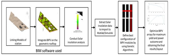
Figure 3.
Sequence of modelling the building-integrated photovoltaics (BIPV) system.
Autodesk Revit 2020 was used to link the BIM models and simulate the solar insolation. It is considered one of highest-level BIM software tools worldwide and is used for major projects because of its high-quality design and models. The same software can be used to link the models and for solar insolation using a 360 plug-in tool that can simulate solar insolation on certain walls, roofs, objects on hourly, daily, monthly, and annual bases.
The next steps are to extract the insolation data from the BIM software for the BIPV arrays, import them to Matlab/Simulink to assess the differences in solar insolation caused by partial shade, and use a GA optimisation toolbox to determine the best layout and configuration that does not limit the power output. The optimisation process determines the best layout of the configuration and electrical connection in the BIPV array in a shape of matrix to maximise the power output without limiting the current throughout the system as well as to avoid multiple peaks in the I-V and P-V curves, which can produce hot spots and damage to the BIPV system. The process of GA optimisation consists of running several iterations of the BIPV arrays in a shape of matrix that depends on the areas of the modelled station. That will allow us to examine all the possible layouts and determine the optimised layout by levelling up the currents in the rows of the BIPV arrays to equalise the currents in the rows. Figure 3 describes the sequence of the adapted methodology.
4. Results
4.1. Integration of BIPV on the Station Rooftop and Solar Feasibility Analysis
Our model mainly focuses on the rooftop in examining the feasibility of installing BIPV on the rooftop of the station. In the BIM software, it is useful to clarify the real-world location of the object modelled. In our case, this is the Education City station, which is located near Al-Rayyan city within Doha metropolitan area. In addition, the software simulates the sun’s movement, which enables us to determine the insolation values based on the exact latitude and longitude of the city’s location in BIM. After that, the solar insolation analysis was performed, which allowed us to draw the layout for segregating the system. In the Appendix A Figure A1 reflect the solar insolation simulation process.
Figure 4 shows the different insolation values of the BIPV modules integrated with the rooftop of the station. It shows the three main levels of insolation on this rooftop. However, Figure 5 illustrates the different areas of directive solar insolation. There are variations in the solar insolation along the rooftop due to the orientation and coordinates of the station and the shape of the rooftop. Each area has its own value of solar insolation.
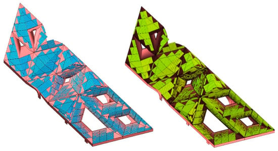
Figure 4.
The BIPV modules are analysed on the rooftop of the station, which has several solar insolation values. The blue (before solar simulation) and green (after solar simulation) colours are BIPV objects, while the pink (before solar simulation) and dark red (after solar simulation) are the roof of the station.
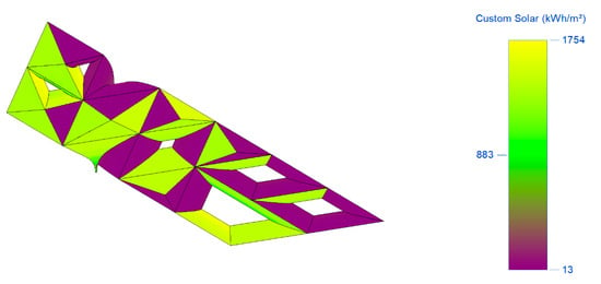
Figure 5.
The rooftop of the station is analysed using a colour gradient, which shows the variation in solar insolation levels. As shown, yellow indicates the areas with the highest solar insolation values. Green indicates the areas with medium solar insolation values. Purple indicates the areas with the lowest solar insolation values.
Figure 6 and Figure 7 show that the station’s rooftop has a high potential for solar energy production. It is clear that the solar insolation through summer, from May to September, is the highest. May has the highest insolation value, producing 969,399 Wh for the entire area of the rooftop, which is 3862 m2. This is equivalent to 251 Wh/m2. In contrast, the lowest insolation value was in December, with an average value of 383,895 Wh for the entire area, or 99 Wh/m2. In Figure 6, the numbers represent the average solar insolation values per m2, while Figure 7 shows the average insolation values for the whole area of the station, as applied in Figure 8 and Figure 9 for the cumulative solar insolation values. The cumulative insolation values for each month are pointed out in Figure 8 and Figure 9. The figures show that May has the highest potential for generating solar energy. The cumulative insolation for the entire area of the rooftop in May is 369,645,427 Wh. December has the lowest potential for generating solar energy, as it has the lowest insolation value of 108,069,467 Wh, which is nearly 30% of the total solar insolation in May. However, as is indicated in Table 2, the whole year achieves a cumulative insolation value of 3,117,787,175 Wh, and the average insolation value for the year is 204 Wh. Moreover, the whole year is included in the averaged and cumulative values, which means that the results of the solar insolation values are applicable to all years.
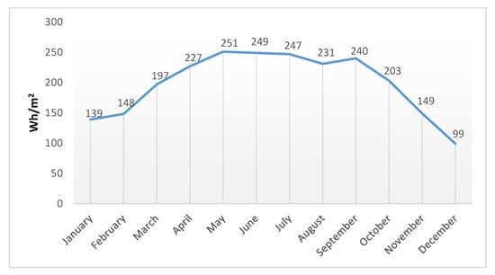
Figure 6.
Average insolation per square metre per month on the rooftop of the station.
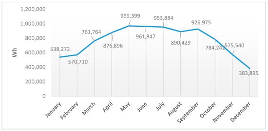
Figure 7.
Average insolation values for the whole rooftop of the station per month.
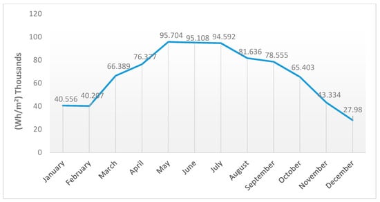
Figure 8.
Cumulative insolation per square metre per month on the rooftop of the station.
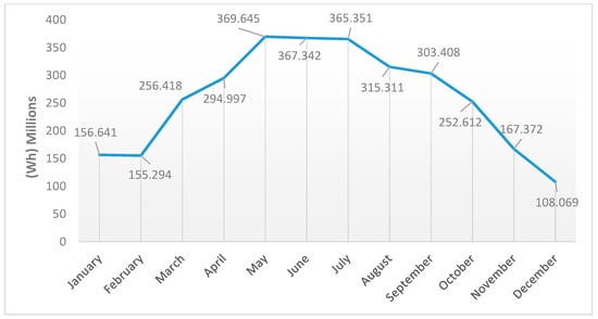
Figure 9.
Cumulative insolation value for the whole area of the station per month.
Table 2.
Yearly (2019) insolation values of the Education City station rooftop.
The solar analysis was conducted for the rooftop of the station for each month during 2019. The results showed great solar potential for the rooftop even though some areas of the rooftop have low insolation levels due to the roof’s curves.
However, to start simulating the insolation values for the station’s rooftop, the rooftop of the station must be segmented because it has multiple curvatures. Each curvature was considered as one area. Segmentation of areas of the station’s rooftop is shown in Figure 10. The station’s rooftop has multiple shapes, and each shape was considered to be a separate area. This was done due to the multiple curvatures in the shape of the rooftop and their corresponding variety of solar insolation values. The photocurrent is directly proportional to the insolation value, and the lowest insolation value in the system can control and limit the whole system’s photocurrent value. Consequently, we need to analyse each area individually to predict the areas with low, medium, and high insolation values. An annual simulation of solar insolation was carried out for each area and there were huge differences in the insolation values; for example, the maximum insolation value for A22 and A23 was 421 Wh/m2 for the whole year, while in A16, the average insolation value was 4.32 Wh/m2. These numbers indicate a large difference in solar insolation across the rooftop and that the complexity of identifying the best configuration for the BIPV system comes from identifying the areas which have low, medium, and high insolation values. These variations are mainly due to the curvatures, which create partial shade. The reason for choosing the average annual solar insolation is that the configuration of the BIPV arrays will be static. Thus, the average annual solar insolation values ensure that all solar insolation values in all months are considered and that this configuration is fitted in over the whole year.
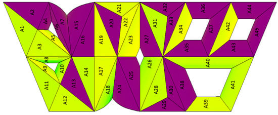
Figure 10.
The rooftop of the station is separated into 45 areas.
As shown in Figure 10, the rooftop of the station was divided into 45 main areas, and each area’s insolation value was modelled across an entire year. Each area can have a certain number of BIPV modules installed upon it. The module chosen for our case study is the Xunlight XRS18-146, which has a surface area of 2.12 m2. In terms of spacing between BIPV modules and arrays, it has been discussed in [45] that spacing between the arrays’ rows impacts their power output because of shade created by them. However, in our case, the BIPV will be directly integrated with the roof and there will be no mounted arrays that can create shade. Therefore, 20% of the surface area of each area can be eliminated for measurement, fittings, edges, connection, and maintenance purposes so long as there is no sufficient spacing studies conducted for BIPV applications. Finally, the number of modules was given for each area in the same table. The colour gradient in Figure 10 is the same as in Figure 5. Yellow indicates the areas with the highest solar insolation values. Green indicates the areas with medium solar insolation values. Purple indicates the areas with the lowest solar insolation values.
Table 3 shows the different classifications for each area and how many BIPV modules can be installed in these areas. These areas are classified into five main insolation categories, as illustrated in Table 4. The categories represent the areas’ insolation values from low to high. Category 1 refers to the areas with insolation values of 0 < x < 10 Wh/m2. Category 2 refers to the areas with insolation values of 10 ≤ x < 300 Wh/m2. Category 3 represents the areas with insolation values of 300 ≤ x < 350 Wh/m2. Category 4 represents the areas with insolation values of 350 ≤ x < 400 Wh/m2. Category 5 refers to the areas with insolation values of 400 Wh/m2 and above.
Table 3.
Specification of area and solar insolation for each area.
Table 4.
Number of BIPV modules for each category.
There is great potential for installing many BIPV modules for each category, but the main issue will be how to electrically connect the modules of each category. This should be done using an optimisation method that allows us to determine the best configuration and layout for the system.
Figure 1, Figure 2, Figure 3, Figure 4, Figure 5, Figure 6, Figure 7, Figure 8 and Figure 9 were created to illustrate the integration of the BIPV modules on the selected building for the study using the BIM tool. Then, based on the average annual solar irradiance at the selected building location, the building’s rooftop was classified into 45 zones. These solar insolation classifications will act as inputs for the GA optimisation algorithm which will optimally configure the physical connections between the 45 zones. In Section 4.2, the 45 BIPV array configurations will be modelled and analysed for optimum power extraction under the partial shading condition and different solar insolation values.
4.2. Optimise the Classified Areas of BIPV for Maximum Power Extraction Using Genetic Algorithms
Based on the analysis of the shading pattern on the roof of the station, it is clear that there is a great difference between the irradiance levels of the areas. These differences will lead to mismatch losses throughout the system if they are connected without considering the partial shading of the BIPV, which causes multiple peaks in the 1–5 and P-V curves that disturb the system. However, to minimise and eliminate these effects within the proposed BIPV system, the rows of the system should be equalised to nearly the same current, and areas should be interconnected based on their solar insolation, as solar insolation plays a key role in generating the current in these different areas. The BIPV module locations will be unchanged, but the interconnections between these areas will be changed based on their solar insolation to make the whole rows have the same solar insolation, which will result in a stabilised BIPV system and maximised power.
The TCT configuration is configured in the circuit by connecting cross ties across each row in a simple Series-Parallel (SP) configuration. In this configuration, the rows are connected in parallel and the columns are connected in series. In this case, the voltage outcome will result from the columns, and the current will result from the rows. As the current relies on the irradiance value, all rows need to be equalised for nearly the same total solar insolation to minimise and eliminate the mismatch losses and the multiple peaks. Otherwise, the BIPV area with the lowest solar insolation will limit the current of the string [46]. Both studies prove that using a GA method for optimising the system performed best and enhanced the stabilisation of the system as reflected by the power output of the modules. The two studies were initiated with 9 × 9 matrices with 81 PV modules. Each row consisted of nine PV modules and each column consisted of nine PV modules [32,36].
The same matrix, interconnection, and optimisation approaches were adopted in our study, but our data were obtained from the solar insolation simulation used in BIM, as we had 45 different areas and each area had multiple PV modules with the same solar insolation. Thus, the whole area was treated as one BIPV module and the total solar insolation of the BIPV modules was taken. The following are illustrations of the BIPV system connections and matrix implemented in our paper.
As shown in Figure 11, the configuration of our system was modified by connecting them in a series and a parallel configuration, and cross ties are connected across each row of the system. The system in Figure 11 can be illustrated in matrix form of which two matrix connections will be considered, as we have 45 areas. Therefore, firstly, the BIPV system was considered for the 5 × 9 matrix. Secondly, the 9 × 5 matrix was tested to analyse both matrices, as the voltage and current values changed. Inside each area, the modules that have the same solar insolation values were connected in series. The current and voltage in the optimisation process can be expressed as follows:
where I is the current, Im is the current in a specific module under specific solar insolation equal to K = G/G0 (G0 = 1000 W/m2). Va is the voltage across the array, and Vmk is the voltage in a specific module [32,36]. Figure 12 illustrates the matrix connection for both systems.
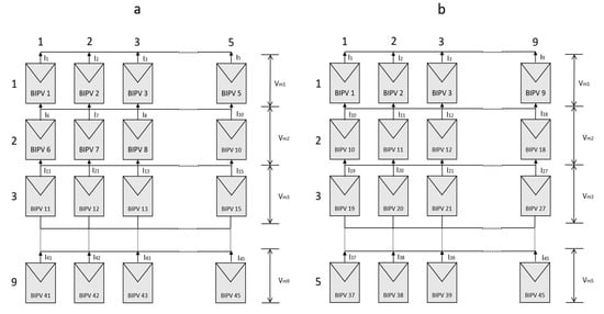
Figure 11.
BIPV system connected in Total Cross-Tied (TCT) configuration with a simple Series-Parallel connection; (a) 5 × 9 connected system, (b) 9 × 5 connected system.
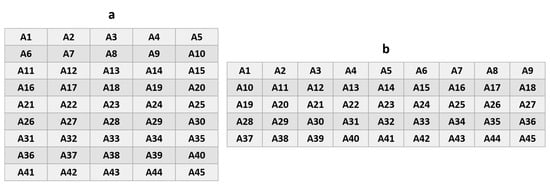
Figure 12.
(a) Matrix interconnection (5 × 9), (b) matrix interconnection (9 × 5).
The following steps needed to be performed to begin the optimisation process. Previous studies proved that GA optimisation enhanced the stabilisation of the PV modules and their power extraction. Consequently, we adopted a GA optimisation method.
A GA can be used in our case because we have changing environmental conditions. Rajan et al. (2017) developed a new GA technique relative to a previous technique developed by Deshkar et al. (2015), and both used the matrix approach [32,36]. Rajan el al.’s (2017) GA technique is less complex, which involves minimising the standard deviation of the row currents. A standard deviation is the average amount of variation within a set of values. A low standard deviation means the values are close to the average of the set while a high standard deviation value indicates that the values comprise a wide range of values that deviate from the average. The GA standard-deviation-based optimisation focuses on minimising the value of the standard deviation of the row currents using the solar insolation data. Minimising the standard deviation values of row currents enhances the stabilisation of the BIPV array and eliminates the multiple peaks and thus maximises extracted power.
The above problem needs to be formulated to define the objective function of the BIPV arrays associated with the BIPV system of the 45 areas to minimise the standard deviation of the row currents, which depends on the individual rows current values. The objective function is,
where, fitness(i) is the fitness of the ith element in the current population.
where σ1 is the standard deviation of individual row currents and N is the number of rows.
where Ij is the current of the jth row.
The GA code is implemented in Matlab where the optimisation process was conducted. The first phase was the initialisation, where the initial population for the first iteration was selected. The population was the 9 × 5 and 5 × 9 matrices, and each population contained the values of these matrices. As the values of the matrices’ elements were already defined as in Figure 13 and they corresponded to the locations in Figure 12, values were rearranged to evaluate the values of the standard deviation for each matrix to find the smallest standard deviation. Then, in the crossover, the values of the 9 × 5 and 5 × 9 matrices were interchanged with other matrices in the population. The next step was the mutation, where the elements inside the matrix were interchanged for a certain probability value. After this step, standard deviation was evaluated for all matrices stored to find the matrix with the lowest standard deviation. After doing so, the first iteration was finished. After selecting the best resulted matrix in the first iteration, the next iteration took place and so on.
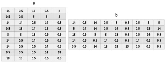
Figure 13.
(a) Matrix interconnection (5 × 9) with the values for each area, (b) 9 × 5 matrix interconnection with the values for each area.
The GA optimisation process was performed for both matrices to find the best outcome (minimum) standard deviation for the summation of the matrices’ rows. Figure 14 shows the iteration progress of the GA optimisation method in identifying the best solution after 100 iterations.
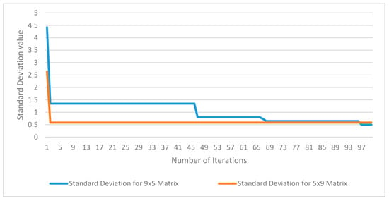
Figure 14.
Value of optimised SD value for both matrices after 100 iterations.
The GA technique was reconfigured to the BIPV arrays which were subject to partial shading and the results equalised the pattern of the interconnection between the areas based on their solar insolation to uniformly distribute the partial shading across all the areas. The currents in the rows were the following:
For the 9 × 5 matrix:
Ir1 = Ir2 = Ir3 = Ir5 = 3 × 0.5 I + 1 × 18 I + 1 × 14 I = 33.5 I;
Ir4 = Ir7 = Ir8 = 2 × 0.5 I + 2 × 14 I + 1 × 5 I = 34 I;
Ir6 = 2 × 0.5 I + 2 × 8 + 1 I × 18 I = 35 I;
Ir9 = 2 × 0.5 I + 2 × 14 I + 1 × 8 I = 37 I.
For the 5 × 9 matrix:
Ir1 = Ir2 = Ir3 = 4 × 0.5 I + 2 × 14 I + 1 × 5 I + 1 × 8 I + 1 × 18 I = 61 I;
Ir4 = Ir5 = 5 × 0.5 + 3 × 14 + 1 × 18 = 62.5 I.
There were 100 iterations for both matrices, and afterwards, the standard deviations for the 9×5 matrix and the 5 × 9 matrix were 0.4969 I and 0.5831 I, respectively. Both the I-V and P-V curves show that the mismatch losses and the multiple peaks were reduced, and this affected the power extraction of the BIPV arrays. For the 9 × 5 matrix BIPV arrays, the current based on the solar insolation was equalised in rows one, two, three, and four with 33.5 kWh/m2 of annual average solar insolation of current in each row. Rows four, seven, and eight had a 34 kWh/m2 of annual average solar insolation, and rows six and nine had 35 kWh/m2 and 37 kWh/m2 of annual solar insolation, respectively. For the 5 × 9 matrix arrays, the solar insolation was equalised more than the 9 × 5 array because it had more element spaces in the rows. Rows one, two, and three had 61 kWh/m2 of annual average solar insolation each, and rows four and five had 62.5 kWh/m2 of annual average solar insolation. Figure 15 shows the minimised standard deviations of each row’s summation.
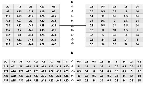
Figure 15.
Reconfiguration of the BIPV system using the Genetic Algorithm (GA) optimisation technique. (a) The 9 × 5 BIPV array reconfiguration result, (b) the 5 × 9 BIPV array reconfiguration result.
When the GA optimisation was completed for equalising the rows, power extraction was simulated for both BIPV arrays, and it was found that the average annual power extraction for the 9×5 array as reflected in Table 5 was 169.6 × 10³ W of average power during the year while the power extraction for the 5×9 array was 169.4 × 10³ W of average power during the year, as illustrated in Figure 16. Optimal results of I-V and P-V curves for both BIPV system configurations. The two charts at the top show the results for the 9 × 5 BIPV array reconfiguration. The two charts at the bottom show the results for the 5 × 9 BIPV array reconfiguration.
Table 5.
Power output, current, and voltage modelled in Simulink based on the GA configuration of distributing equalised solar insolation within the 9 × 5 and 5 × 9 BIPV arrays.
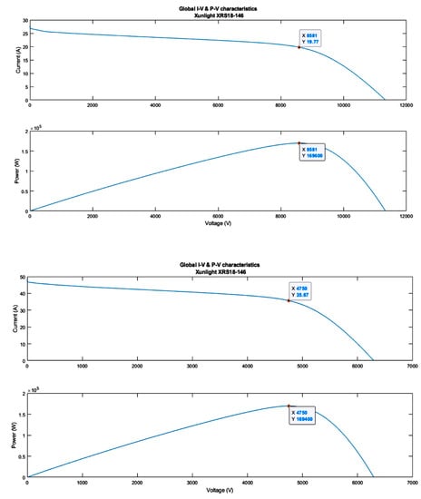
Figure 16.
Optimal results of I-V and P-V curves for both BIPV system configurations. The two charts at the top show the results for the 9 × 5 BIPV array reconfiguration. The two charts at the bottom show the results for the 5 × 9 BIPV array reconfiguration.
The small difference in power between both matrices is because, in the 5 × 9 matrix, there is more series connection with more solar insolation differences, which causes more current limitation than in the 9 × 5 matrix. Moreover, the curves of both systems reveal that the GA optimisation method succeeded in equalising the rows to stabilise the BIPV system and to reach the global power extraction without any disturbance or multiple peaks.
5. Discussion
This paper presented a novel methodology for integrating BIM tools with a GA optimisation technique. The results showed a great possibility for power production, as the cumulative solar insolation for the year was 3,117,787,175 Wh for the whole area of the station’s roof of 3862 m2. The greatest solar insolation values were found in the summer (May–August), while the lowest solar insolation values were found in the winter (November–February). Due to the difference in solar insolation values in the 45 areas of the roof, which are caused by the curvatures of the roof, the performance of the BIPV system arrays is disturbed by partial shading. The GA optimisation technique was used to start arranging the BIPV arrays based on solar insolation values by equalising the solar insolation values in each row of the two proposed BIPV matrix arrangement. In [28] and [37], BIM tools associated with predicting the energy production of the two models were based on the solar insolation values. However, in these studies, there was no partial shading. Consequently, there was no difference in solar insolation values, and the roofs of these models were aligned in a straight manner. By contrast, we had to solve the partial shading issue using an optimisation method, as the BIPV arrays need to be connected in a way that maximises their power extraction under partial shading conditions. The partial shading problem was solved in both [32] and [36] using a GA optimisation method that equalises the rows with the same solar insolation values in a 9 × 9 matrix. However, the solar insolation values in both studies were based on assumptions. The contribution of this work was solving the partial shading problem and dealing with the difference in solar insolation values by importing the results from a BIM tool using the simulated solar insolation values from the actual site location. Moreover, the GA optimisation method was used to best connect the BIPV arrays for the 45 areas in 9 × 5 and 5 × 9 matrix shapes in order to maximise the power extraction of their BIPV modules. The system’s component was not included in this paper. This paper solves the problem of the partial shading condition on the BIPV and designs the system based on the solar insolation values of the BIPV so as to not limit the current in the system by using GA optimisation. The system’s component and grid connectivity issues will be discussed in our next paper. The optimisation problem in this article aims to determine the optimum power generation of the BIPV system under partial shading conditions. The existing design of the roof and the solar insolation values represent the optimisation problem constraints. The authors have excluded the demand-side of the station as it will not impact the results. In addition, it is notable that the station’s operation started less than a year ago and remained under commission during the first two years. The authors are planning to include the station’s load profile in a future work when full-year reliable data are available. The curves shown in Figure 16 confirm the improvement in the system’s stability and the achievement of the objective of this article to design the BIPV arrays for maximum power production under partial shading conditions without any disturbance to the system. Furthermore, the installation is only done once in the design phase and is based on the resulting system configuration throughout the year. The wire layout can also be optimised to limit current loops and the cables can be shortened.
6. Conclusions
The concept being adopted is to implement renewable energy technology in one of the most recent major projects in Qatar to mitigate pollution (environmental benefit) and conserve energy sources for export and other uses (economic benefit). The first stage of this paper was to model the station using the BIM software Autodesk Revit and create BIPV modules on the roof of the station. The station’s roof is geometrically complex, as there are many curvatures, which can cause partial shading that can disturb the BIPV system arrays. The station’s roof was divided into 45 areas and the average yearly solar insolation was simulated for each. These values where used in the GA optimisation process to eliminate differences in the solar insolation values caused by partial shading by uniformly distributing the shading pattern across the areas. Two BIPV array configurations were considered, 9 × 5 and 5 × 9 BIPV system configurations, whose optimisation required the minimisation of the standard deviation of the summation of their rows. This process was conducted to stabilise the current in the rows and eliminate the multiple peaks and the mismatch losses. The power output was modelled in Simulink for which the power for the 9 × 5 BIPV array was 169.6 × 10³ W, which was slightly higher than the 5 × 9 BIPV array’s power output. This is a sign that the GA optimisation method using the actual solar insolation values of the BIPV system succeeded in reaching the global optimum power without any disturbance to the system. In conclusion, the paper has proposed a new methodology for integrating BIM with GA optimisation to mitigate and solve the issue of partial shading. In addition, this paper proposes that Qatar integrates renewables into major projects for energy, economic, and environmental benefits.
Author Contributions
Conceptualisation, S.A.A.-J., O.E. and S.G.A.-G.; Formal analysis, S.A.A.-J.; Funding acquisition, S.G.A.-G.; Investigation, S.A.A.-J.; Methodology, S.A.A.-J., O.E. and S.G.A.-G.; Project administration, S.G.A.-G.; Supervision, S.G.A.-G.; Visualisation, S.A.A.-J., S.G.A.-G.; Writing—original draft, S.A.A.-J.; Writing—review and editing, O.E. and S.G.A.-G. All authors have read and agreed to the published version of the manuscript.
Funding
The publication of this article was funded by the Qatar National Library.
Acknowledgments
This research was supported by a scholarship from Hamad Bin Khalifa University (HBKU) a member of the Qatar Foundation (QF). Any opinions, findings, and conclusions or recommendations expressed in this material are those of the author(s) and do not necessarily reflect the views of HBKU or QF.
Conflicts of Interest
The authors declare no conflict of interest.
Appendix A

Figure A1.
Top view of the sun movement over the station building in the BIM environment. This is precisely for the case study building in Al-Rayyan city within Doha metropolitan, Qatar. The sun is shown here at 9:15 a.m. on 15 March. The shaded yellow area represents an example of the sun movement range from 15 March to 31 December, from 9:15 a.m. to 3:00 p.m., although, as shown, the sunrise is at 5:43 a.m. and the sunset is at 5:42 p.m. In our analysis, we accounted for the whole year from sunrise to sunset.

The equations of PV cell modelling can be expressed as follows [42,43]:
However, the photocurrent depends on the solar insolation, which can be absorbed by the PV cell. The equation below expresses that the solar insolation and operating temperature are the key factors for the photocurrent:
Isc represents the short circuit current (A), KI is the temperature coefficient for the short-circuit current, TRef is the cell’s reference temperature (273.15 K), and λ is the solar insolation in kW/m2. However, the equation of saturation current can be obtained from the equation below:
IRS represents the reverse saturation current (A) at reference temperature and insolation, and EG is the band-gap energy of the semiconductor used in the cell (eV). For silicon, EG = 1.17 eV. The reverse saturation current can be obtained by
where VOC represents the open-circuit voltage.
Commonly, the PV cell is unaffected by different values of RSH in the cell, which can be neglected. However, any small change in RS will cause a large change in the cell’s power output. Therefore, the equation of the PV cell model can be made less complex as follows:
For the PV cell to operate ideally, there should be no RS or leakage of current. Therefore, the PV model equation can be simplified according to the following equation:
The developed model is a simplified model based on the mentioned equations. However, the modelling equation for an a-Si cell type and the current-voltage generated can be represented in the equation below [47]:
where di represents the thickness of i-layer in the BIPV module, the effective product μτeff represents the average lifetime for election and hole and quantify the quality of the active layer, Vbi represents the built-in field voltage over i-layer, VT represents the thermal voltage.
References
- Martín-Pomares, L.; Martínez, D.; Polo, J.; Perez-Astudillo, D.; Bachour, D.; Sanfilippo, A. Analysis of the long-term solar potential for electricity generation in Qatar. Renew. Sustain. Energy Rev. 2017, 73, 1231–1246. [Google Scholar] [CrossRef]
- Razykov, T.M.; Ferekides, C.S.; Morel, D.; Stefanakos, E.; Ullal, H.S.; Upadhyaya, H.M. Solar photovoltaic electricity: Current status and future prospects. Sol. Energy 2011, 85, 1580–1608. [Google Scholar] [CrossRef]
- Kamal, A.; Al-Ghamdi, S.G.; Koc, M. Building Stock Inertia and Impacts on Energy Consumption and CO2 Emissions in Qatar. In Proceedings of the ASME 2019 13th International Conference Energy Sustainability, Bellevue, WA, USA, 14–17 July 2019. [Google Scholar] [CrossRef]
- Weber, A.S. Review of sustainable and renewable energy activities in the state of Qatar. In Proceedings of the 2013 International Renewable and Sustainable Energy Conference (IRSEC), Ouarzazate, Morocco, 7–9 March 2013; pp. 91–95. [Google Scholar]
- Touati, F.; Al-Hitmi, M.; Bouchech, H. Towards understanding the effects of climatic and environmental factors on solar PV performance in arid desert regions (Qatar) for various PV technologies. In Proceedings of the 2012 First International Conference on Renewable Energies and Vehicular Technology, Hammamet, Tunisia, 26–28 March 2012; pp. 78–83. [Google Scholar]
- Bachour, D.; Perez-Astudillo, D. Ground measurements of Global Horizontal Irradiation in Doha, Qatar. Renew. Energy 2014, 71, 32–36. [Google Scholar] [CrossRef]
- Touati, F.; Gonzales, A.S.P.; Qiblawey, Y.; Benhmed, K. A Customized PV Performance Monitoring System in Qatar’s Harsh Environment. In Proceedings of the 2018 6th International Renewable and Sustainable Energy Conference (IRSEC), Rabat, Morocco, 5–8 December 2018; pp. 1–6. [Google Scholar]
- Government Communications Office (GCO). Qatar National Vision 2030; Government Communications Office: Doha, Qatar, 2008.
- Talavera, A.M.; Al-Ghamdi, S.G.; Koç, M. Sustainability in mega-events: Beyond qatar 2022. Sustainability 2019, 11, 6407. [Google Scholar] [CrossRef]
- Andrić, I.; Le Corre, O.; Lacarrière, B.; Ferrão, P.; Al-Ghamdi, S.G. Initial approximation of the implications for architecture due to climate change. Adv. Build. Energy Res. 2019, 1–31. [Google Scholar] [CrossRef]
- Salimzadeh, N.; Vahdatikhaki, F.; Hammad, A. Parametric modeling and surface-specific sensitivity analysis of PV module layout on building skin using BIM. Energy Build. 2020, 216, 109953. [Google Scholar] [CrossRef]
- Husain, A.A.F.; Hasan, W.Z.W.; Shafie, S.; Hamidon, M.N.; Pandey, S.S. A review of transparent solar photovoltaic technologies. Renew. Sustain. Energy Rev. 2018, 94, 779–791. [Google Scholar] [CrossRef]
- Parida, B.; Iniyan, S.; Goic, R. A review of solar photovoltaic technologies. Renew. Sustain. Energy Rev. 2011, 15, 1625–1636. [Google Scholar] [CrossRef]
- Touati, F.; Massoud, A.; Hamad, J.; Saeed, S.A. Effects of Environmental and Climatic Conditions on PV Efficiency in Qatar. Renew. Energy Power Qual. J. 2013, 262–267. [Google Scholar] [CrossRef]
- Mühlbauer, M. Smart building-integrated photovoltaics (BIPV) for Qatar. QScience Connect 2017, 2017, 3. [Google Scholar] [CrossRef]
- Al-Janahi, S.A.; Ellabban, O.; Al-Ghamdi, S.G. Optimal Configuration for Building Integrated Photovoltaics System to Mitigate the Partial Shading on Complex Geometric Roofs. In Proceedings of the 2019 2nd International Conference on Smart Grid and Renewable Energy (SGRE), Doha, Qatar, 19–21 November 2019; pp. 1–6. [Google Scholar]
- Walker, L.; Hofer, J.; Schlueter, A. High-resolution, parametric BIPV and electrical systems modeling and design. Appl. Energy 2019, 238, 164–179. [Google Scholar] [CrossRef]
- Norton, B.; Eames, P.C.; Mallick, T.K.; Huang, M.J.; McCormack, S.J.; Mondol, J.D.; Yohanis, Y.G. Enhancing the performance of building integrated photovoltaics. Sol. Energy 2011, 85, 1629–1664. [Google Scholar] [CrossRef]
- Seyedmahmoudian, M.; Mekhilef, S.; Rahmani, R.; Yusof, R.; Renani, E. Analytical Modeling of Partially Shaded Photovoltaic Systems. Energies 2013, 6, 128–144. [Google Scholar] [CrossRef]
- Zomer, C.; Nobre, A.; Reindl, T.; Rüther, R. Shading analysis for rooftop BIPV embedded in a high-density environment: A case study in Singapore. Energy Build. 2016, 121, 159–164. [Google Scholar] [CrossRef]
- Gallardo-Saavedra, S.; Karlsson, B. Simulation, validation and analysis of shading effects on a PV system. Sol. Energy 2018, 170, 828–839. [Google Scholar] [CrossRef]
- Al-Ghamdi, S.G.; Bilec, M.M. Green Building Rating Systems and Environmental Impacts of Energy Consumption from an International Perspective. In Proceedings of the International Conference on Sustainable Infrastructure 2014, Long Beach, CA, USA, 6–8 November 2014; pp. 631–640. [Google Scholar] [CrossRef]
- Gui, N.; Qiu, Z.; Gui, W.; Deconinck, G. An integrated design platform for BIPV system considering building information. In Proceedings of the 2017 IEEE Conference on Energy Internet and Energy System Integration (EI2), Beijing, China, 26–28 November 2017; pp. 1–6. [Google Scholar]
- Gupta, A. Developing a BIM-Based Methodology to Support Renewable Energy Assessment of Buildings; Cardiff University: Cardiff, UK, 2013. [Google Scholar]
- Yang, R.J. Overcoming technical barriers and risks in the application of building integrated photovoltaics (BIPV): Hardware and software strategies. Autom. Constr. 2015, 51, 92–102. [Google Scholar] [CrossRef]
- Quintana, S.; Huang, P.; Saini, P.; Zhang, X. A preliminary techno-economic study of a building integrated photovoltaic (BIPV) system for a residential building cluster in Sweden by the integrated toolkit of BIM and PVSITES. Intell. Build. Int. 2020, 1–19. [Google Scholar] [CrossRef]
- Dixit, M.; Yan, W. BIPV Prototype for the Solar Insolation Calculation. In Proceedings of the 29th International Symposium on Automation and Robotics in Construction, Eindhoven, The Netherlands, 26–29 June 2012. [Google Scholar]
- Kuo, H.-J.; Hsieh, S.-H.; Guo, R.-C.; Chan, C.-C. A verification study for energy analysis of BIPV buildings with BIM. Energy Build. 2016, 130, 676–691. [Google Scholar] [CrossRef]
- Freitas, S. Maximizing the Solar Photovoltaic Yield in Different Building Facade Layouts. In Proceedings of the 31st European Photovoltaic Solar Energy Conference and Exhibition, Hamburg, Germany, 14–18 September 2015. [Google Scholar]
- Irwanto, M.; Badlishah, R.; Masri, M.; Irwan, Y.M.; Gomesh, N. Optimization of photovoltaic module electrical characteristics using genetic algorithm (a comparative study between simulation and data sheet of PV Module). In Proceedings of the 2014 IEEE 8th International Power Engineering and Optimization Conference (PEOCO2014), Langkawi, Malaysia, 24–25 March 2014; pp. 532–536. [Google Scholar]
- Sai Krishna, G.; Moger, T. Reconfiguration strategies for reducing partial shading effects in photovoltaic arrays: State of the art. Sol. Energy 2019, 182, 429–452. [Google Scholar] [CrossRef]
- Deshkar, S.N.; Dhale, S.B.; Mukherjee, J.S.; Babu, T.S.; Rajasekar, N. Solar PV array reconfiguration under partial shading conditions for maximum power extraction using genetic algorithm. Renew. Sustain. Energy Rev. 2015, 43, 102–110. [Google Scholar] [CrossRef]
- Ismail, M.S.; Moghavvemi, M.; Mahlia, T.M.I. Characterization of PV panel and global optimization of its model parameters using genetic algorithm. Energy Convers. Manag. 2013, 73, 10–25. [Google Scholar] [CrossRef]
- Alonso Campos, J.C.; Jiménez-Bello, M.A.; Martínez Alzamora, F. Real-time energy optimization of irrigation scheduling by parallel multi-objective genetic algorithms. Agric. Water Manag. 2020, 227, 105857. [Google Scholar] [CrossRef]
- Zhou, Y.; Zhou, N.; Gong, L.; Jiang, M. Prediction of photovoltaic power output based on similar day analysis, genetic algorithm and extreme learning machine. Energy 2020, 117894. [Google Scholar] [CrossRef]
- Rajan, N.A.; Shrikant, K.D.; Dhanalakshmi, B.; Rajasekar, N. Solar PV array reconfiguration using the concept of Standard deviation and Genetic Algorithm. Energy Procedia 2017, 117, 1062–1069. [Google Scholar] [CrossRef]
- Ning, G.; Kan, H.; Zhifeng, Q.; Weihua, G.; Geert, D. e-BIM: A BIM-centric design and analysis software for Building Integrated Photovoltaics. Autom. Constr. 2018, 87, 127–137. [Google Scholar] [CrossRef]
- Qatar Rail. Doha Metro Project. Available online: https://corp.qr.com.qa/ (accessed on 12 February 2020).
- Al-Thawadi, F.E.; Al-Ghamdi, S.G. Evaluation of sustainable urban mobility using comparative environmental life cycle assessment: A case study of Qatar. Transp. Res. Interdiscip. Perspect. 2019, 1, 100003. [Google Scholar] [CrossRef]
- NREL System Advisor Model. Available online: https://sam.nrel.gov (accessed on 25 February 2020).
- PV Module XRS18-146 Details. Available online: http://www.solarhub.com/product-catalog/pv-modules/25289-XRS18-146-Xunlight-Corporation (accessed on 26 February 2020).
- Said, S.; Massoud, A.; Benammar, M.; Ahmed, S. A matlab/simulink based photovoltaic array model employing simpowersystems toolbox. J. Energy Power Eng. 2012, 6, 1965–1975. [Google Scholar]
- Krismadinata; Rahim, N.A.; Ping, H.W.; Selvaraj, J. Photovoltaic Module Modeling using Simulink/Matlab. Procedia Environ. Sci. 2013, 17, 537–546. [Google Scholar] [CrossRef]
- Nguyen, X.H.; Nguyen, M.P. Mathematical modeling of photovoltaic cell/module/arrays with tags in Matlab/Simulink. Environ. Syst. Res. 2015, 4, 24. [Google Scholar] [CrossRef]
- Kanters, J.; Davidsson, H. Mutual Shading of PV Modules on Flat Roofs: A Parametric Study. Energy Procedia 2014, 57, 1706–1715. [Google Scholar] [CrossRef]
- Mayer, M.J.; Gróf, G. Techno-economic optimization of grid-connected, ground-mounted photovoltaic power plants by genetic algorithm based on a comprehensive mathematical model. Sol. Energy 2020, 202, 210–226. [Google Scholar] [CrossRef]
- Louzazni, M.; Khouya, A.; Crăciunescu, A.; Amechnoue, K.; Mussetta, M. Modelling and Parameters Extraction of Flexible Amorphous Silicon Solar Cell a-Si:H. Appl. Sol. Energy 2020, 56, 1–12. [Google Scholar] [CrossRef]


© 2020 by the authors. Licensee MDPI, Basel, Switzerland. This article is an open access article distributed under the terms and conditions of the Creative Commons Attribution (CC BY) license (http://creativecommons.org/licenses/by/4.0/).