Optimal Management of Thermal Comfort and Driving Range in Electric Vehicles

Abstract
1. Introduction
2. State of the Art
2.1. Energy and Thermal Comfort Management Methods
2.2. Thermal Comfort
3. System Description and Modeling
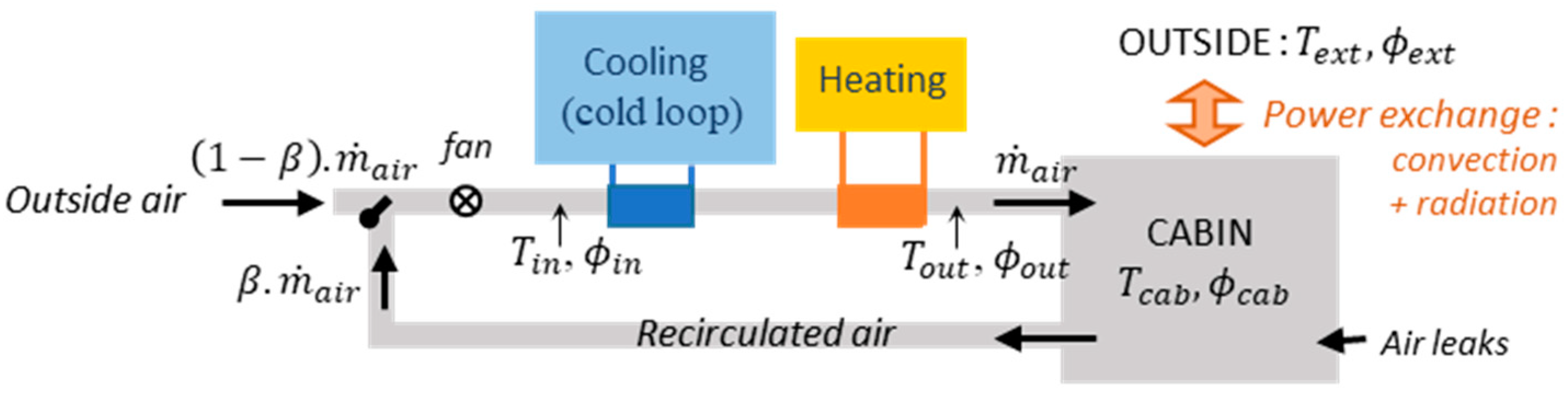
3.1. HVAC System Description and Modeling
3.2. Powertrain Model
3.3. Battery Model
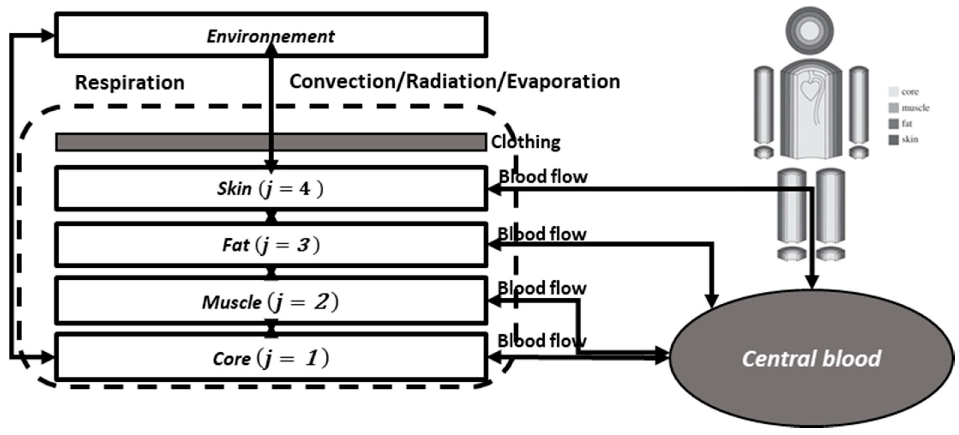
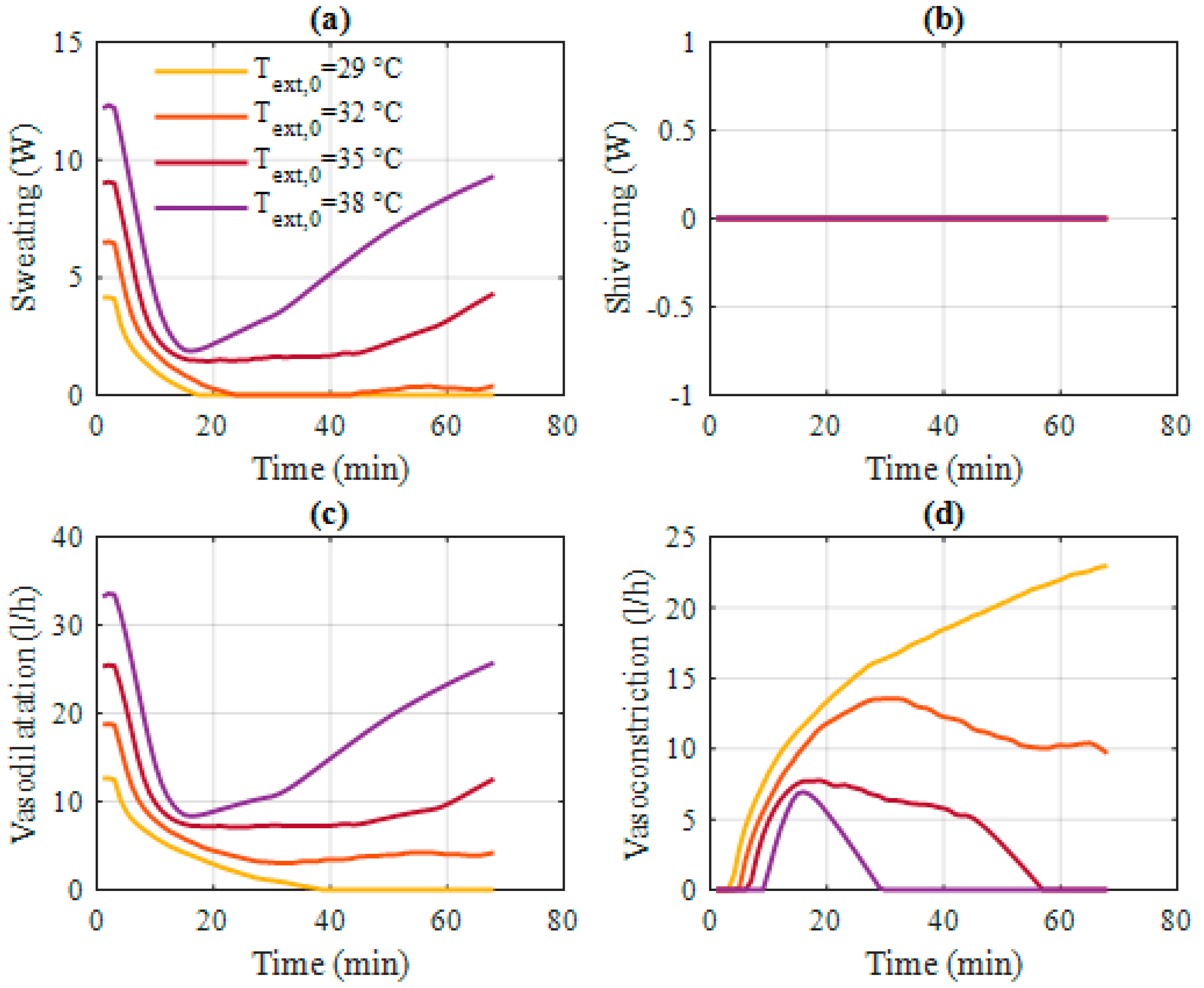
3.4. Thermo-Physiological Model
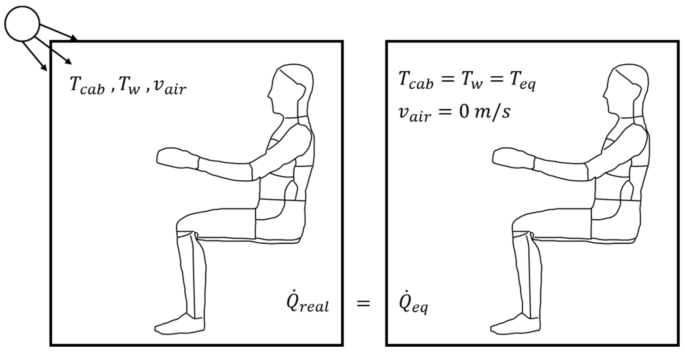
3.5. Thermal Comfort Index
4. Optimal Energy Management
4.1. Cost Function
4.2. Problem Formulation
4.3. Problem Solving by Dynamic Programing
5. Simulation Results
5.1. Simulation Data and Technical Characteristics of the Vehicle
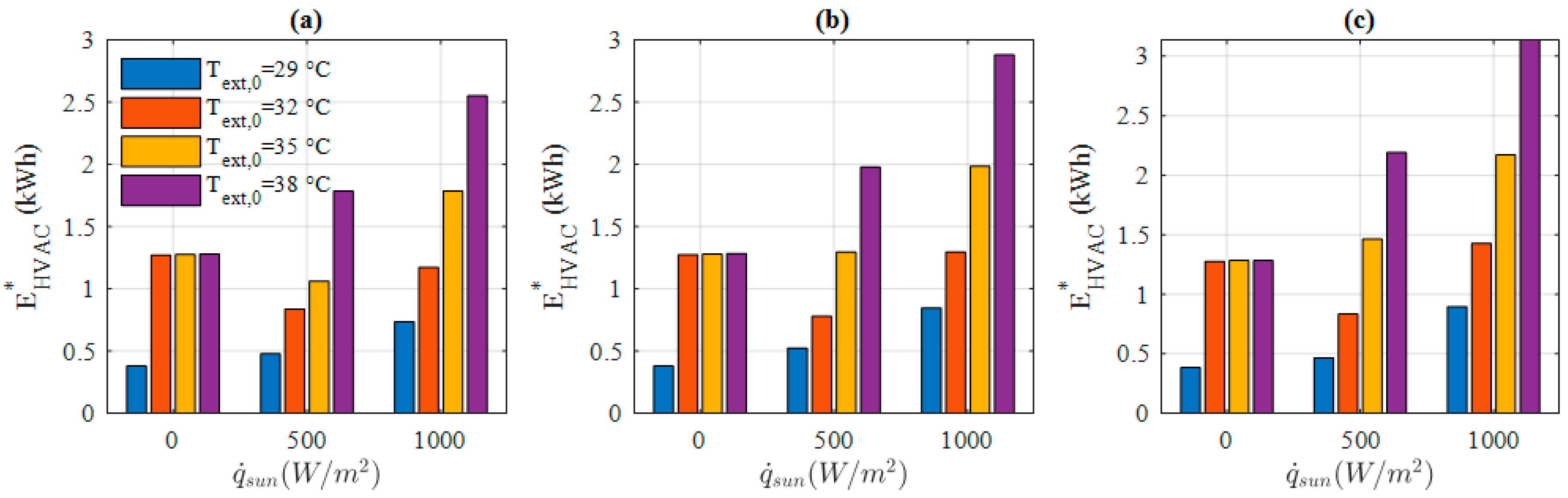
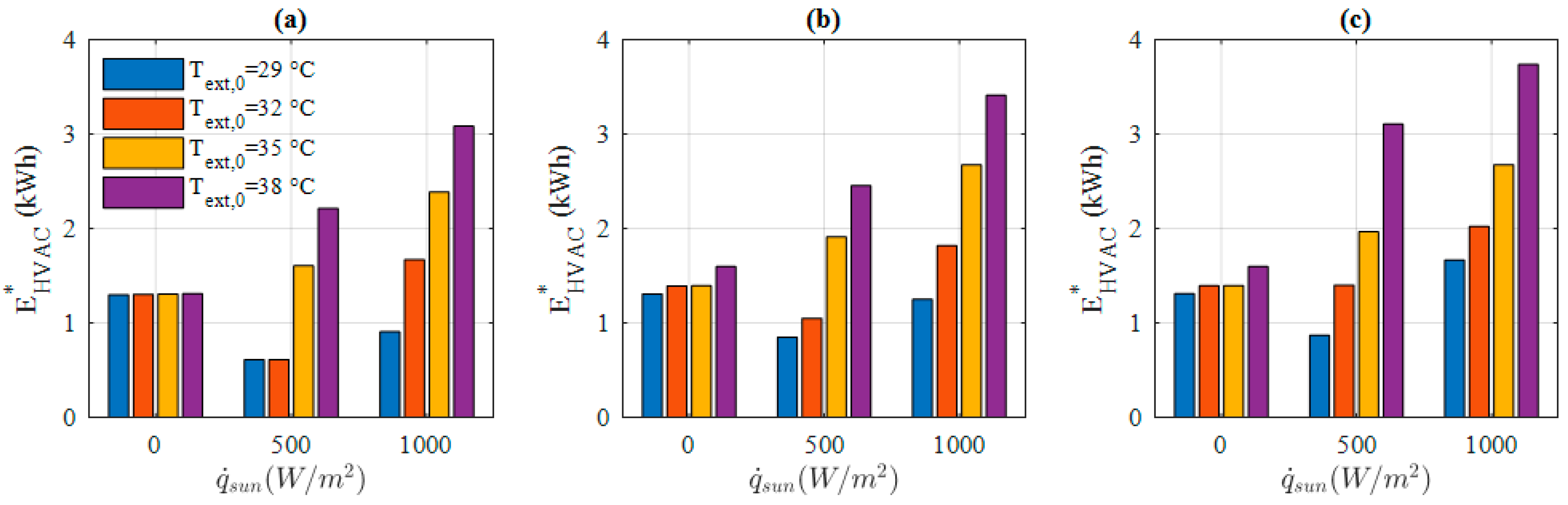
5.2. Ideal Comfort Results
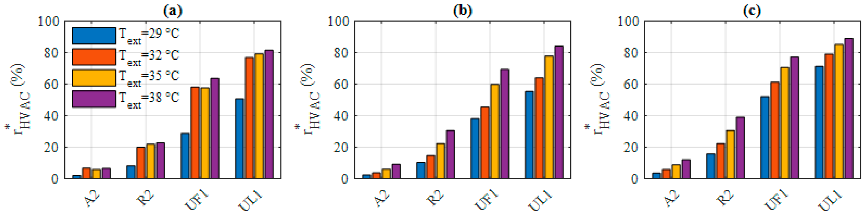
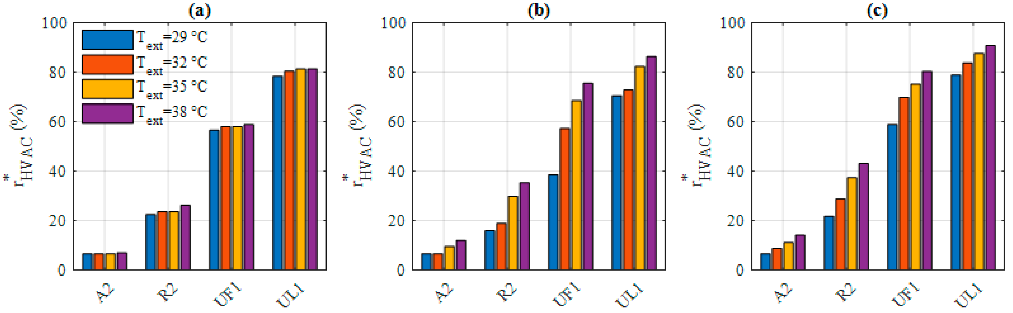
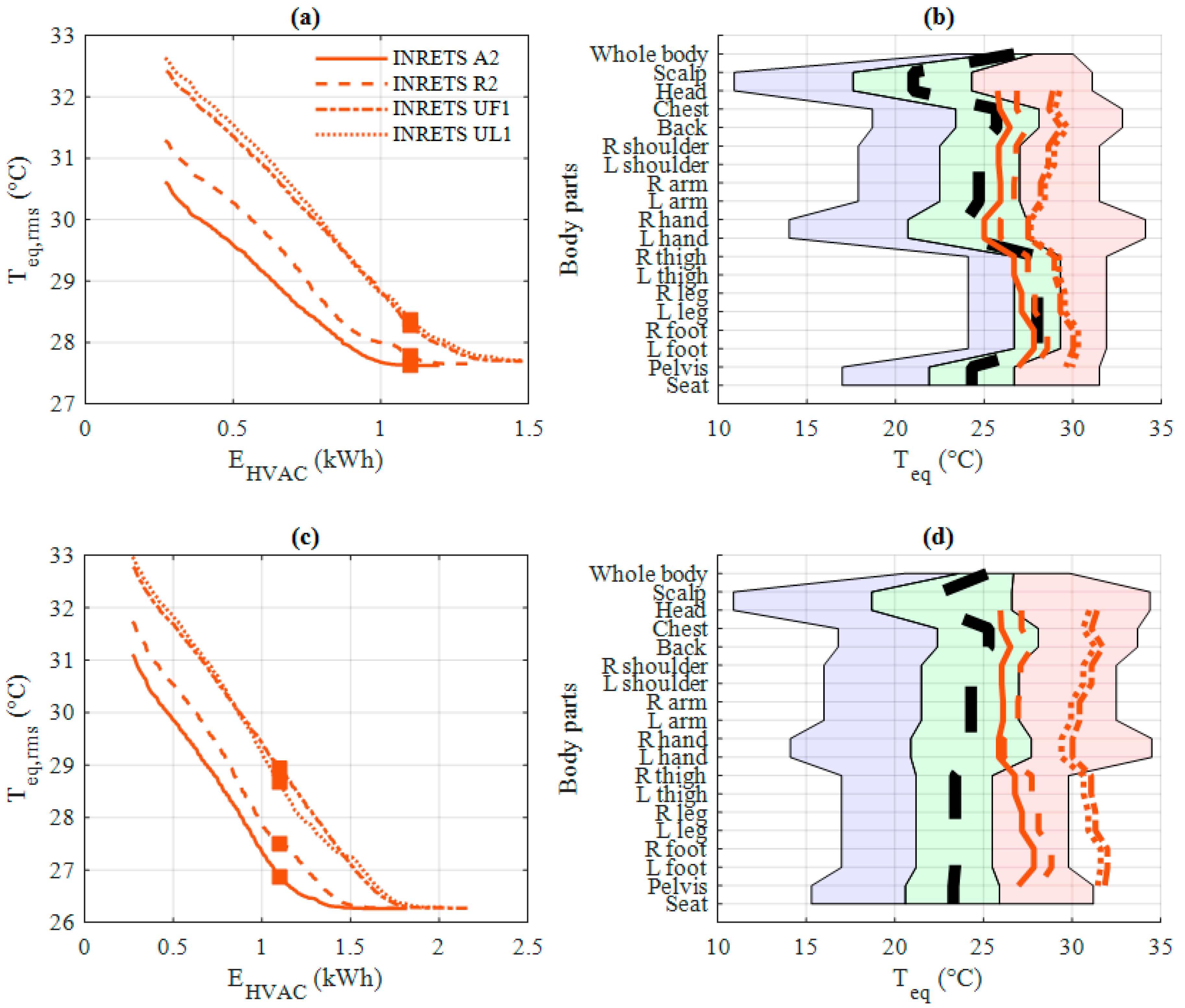
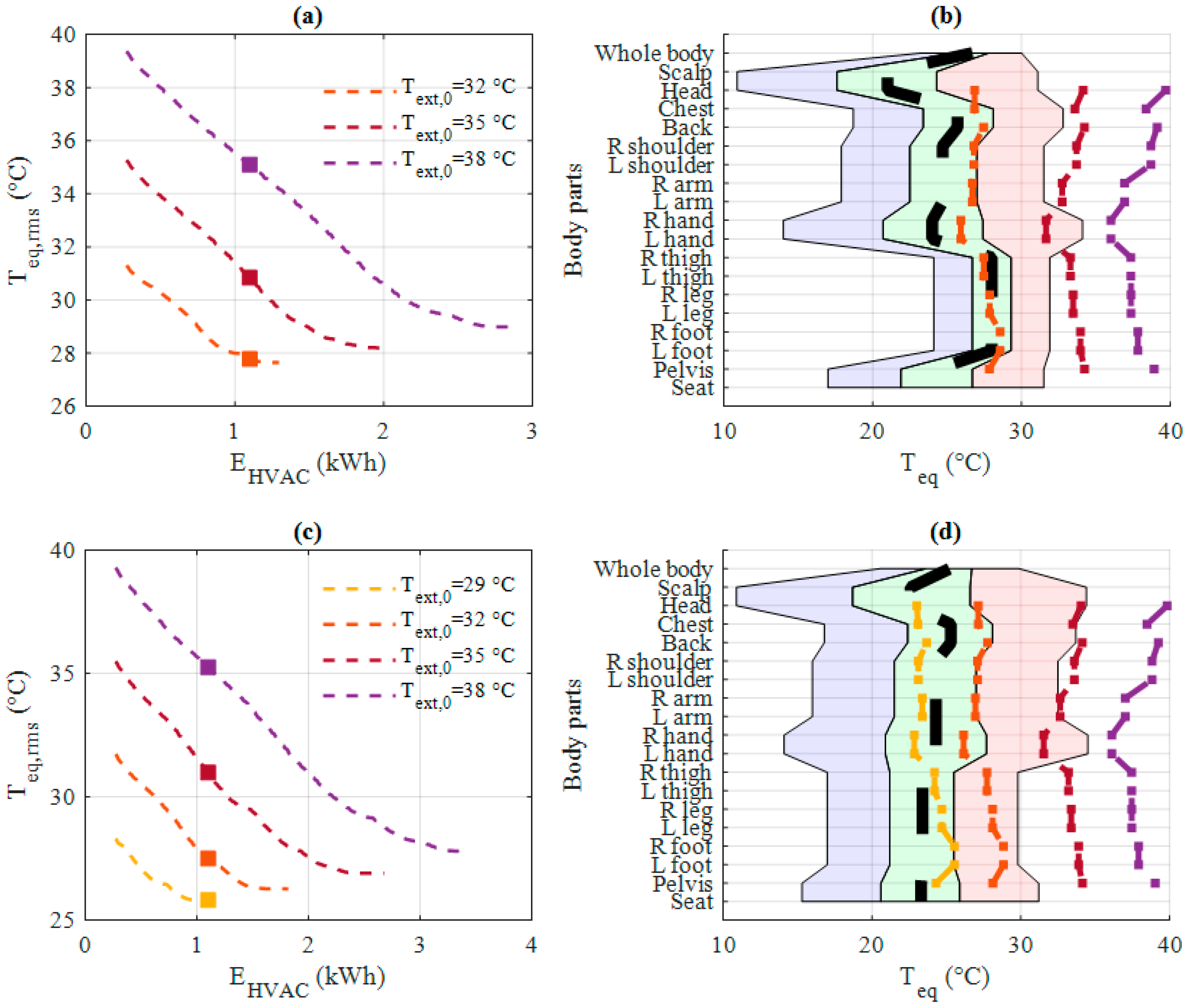
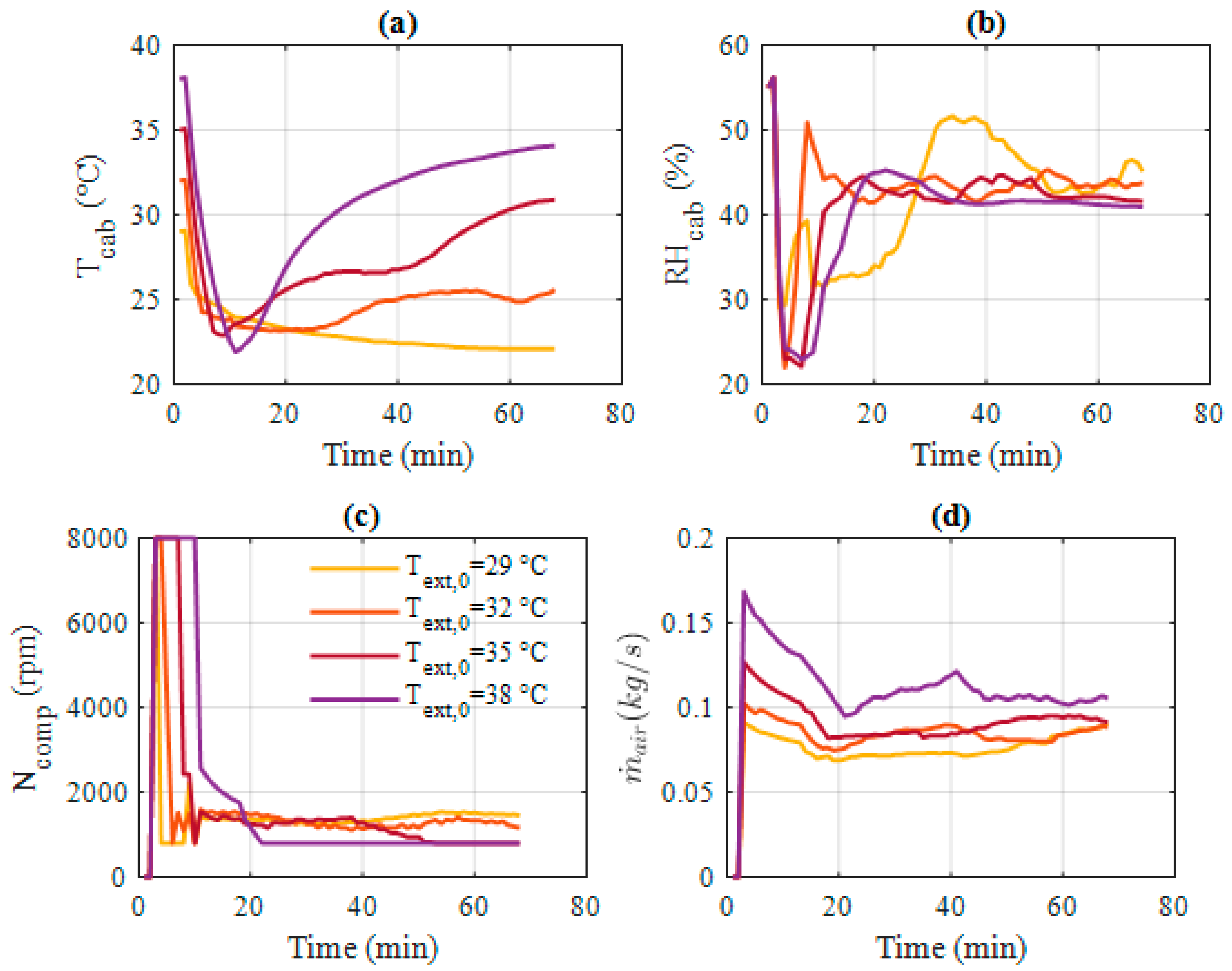
5.3. Test Case 1: Thermal Discomfort vs. Energy Cost Trade-off
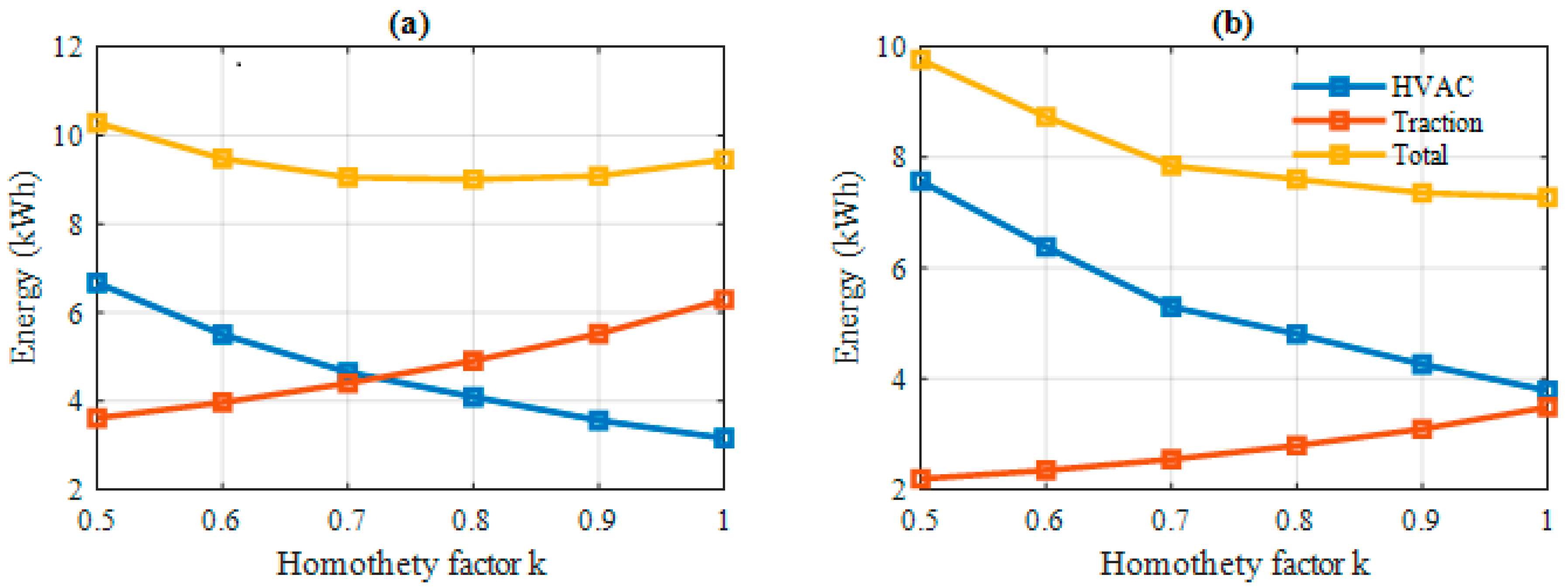
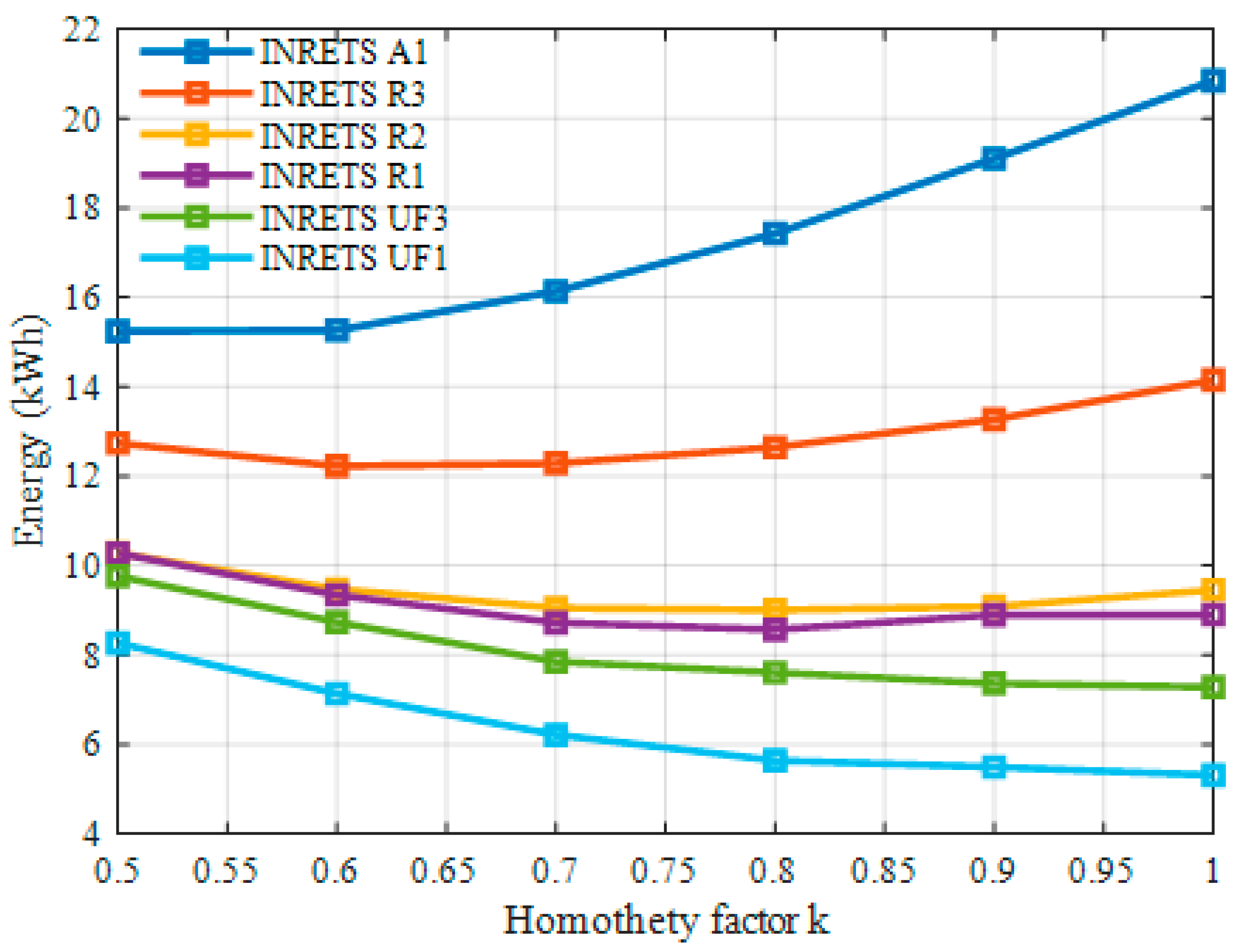
5.4. Test Case 2: Vehicle Speed vs. Thermal Comfort Trade-off
6. Conclusions and Perspectives
Author Contributions
Funding
Acknowledgments
Conflicts of Interest
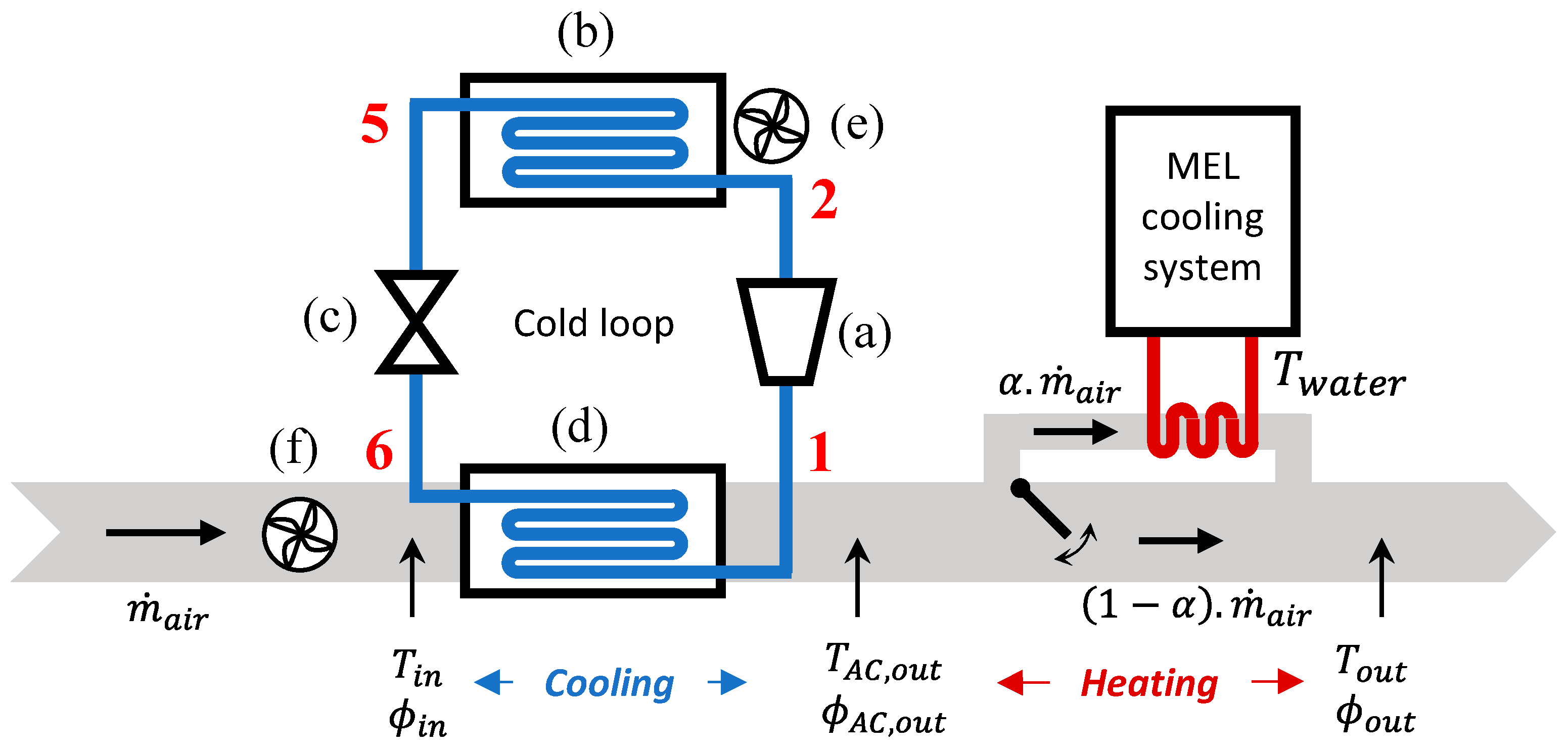
Appendix A. Details of HVAC Modeling
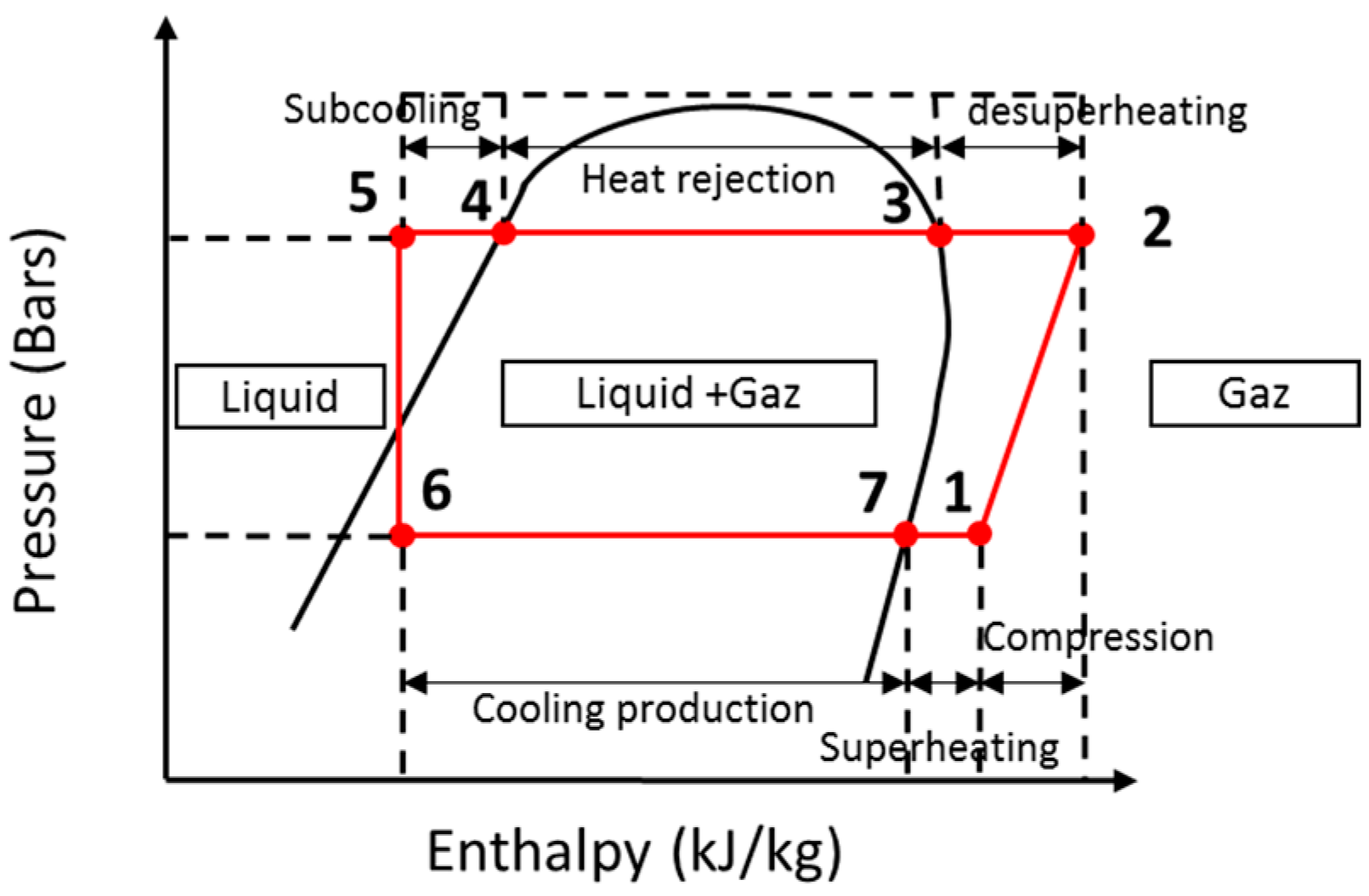
Appendix A.1. Cold Loop Modeling

| Component | Assumptions | Variables | Equations |
|---|---|---|---|
| Cabin | All quantities are spatially uniform | , | (A1), (A2), (A3) |
| Evaporator | Superheating is constant | , | (A8), (9) |
| Valve | The expansion is isenthalpic | (9) | |
| Compressor | Discharge volume is constant | , | (A15), (10) |
| Condenser | Subcooling is constant | , | (A19), (9) |
Appendix A.1.1. Cabin
Appendix A.1.2. Evaporator
Appendix A.1.3. Air Thermal Properties at AC Outlet
Appendix A.1.4. Expansion Valve
Appendix A.1.5. Compressor
Appendix A.1.6. Condenser
Appendix A.2. Heating System Modeling
References
- Lahlou, A.; Ossart, F.; Boudard, E.; Roy, F.; Bakhouya, M. A dynamic programming approach for thermal comfort control in electric vehicles. In Proceedings of the 2018 Vehicle Power and Propulsion Conference (VPPC), Chicago, IL, USA, 27–30 August 2018. [Google Scholar]
- Tanabe, S.; Kobayashi, K.; Nakano, J.; Ozeki, Y. Evaluation of thermal comfort using combined multi-node thermoregulation (65 MN) and radiation models and computational fluid dynamics (CFD). Energy Builds 2002, 34, 637–646. [Google Scholar] [CrossRef]
- He, H.; Wang, C.; Jia, H. A Stochastic model predictive controller based on combined conditions of air conditioning system for electric vehicles. DEStech Trans. Environ. Energy Earth Sci. 2019. [Google Scholar] [CrossRef]
- De Nunzio, G.; Sciarretta, A.; Steiner, A.; Mladek, A. Thermal management optimization of a heat-pump-based HVAC system for cabin conditioning in electric vehicles. In Proceedings of the 2018 Thirteenth International Conference on Ecological Vehicles and Renewable Energies (EVER), Monte-Carlo, Monaco, 10–12 April 2018; pp. 1–7. [Google Scholar]
- He, H.; Jia, H.; Sun, C.; Sun, F. Stochastic model predictive control of air conditioning system for electric vehicles: Sensitivity study, comparison, and improvement. IEEE Trans. Ind. Inform. 2018, 14, 4179–4189. [Google Scholar] [CrossRef]
- Sakhdari, B.; Azad, N.L. An optimal energy management system for battery electric vehicles. IFAC Pap. 2015, 48, 86–92. [Google Scholar] [CrossRef]
- Müller, E.A.; Onder, C.H.; Guzzella, L.; Mann, K. Optimal control of a block heater for an improved vehicle warm-up. IFAC Proc. Vol. 2004, 37, 91–96. [Google Scholar] [CrossRef]
- Müller, E.A.; Onder, C.H.; Guzzella, L.; Kneifel, M. Optimal control of a fuel-fired auxiliary heater for an improved passenger vehicle warm-up. Control Eng. Pract. 2009, 17, 664–675. [Google Scholar] [CrossRef]
- Zhang, Q.; Canova, M. Modeling air conditioning system with storage evaporator for vehicle energy management. Appl. Therm. Eng. 2015, 87, 779–787. [Google Scholar] [CrossRef]
- Mansour, C.; Nader, W.B.; Breque, F.; Haddad, M.; Nemer, M. Assessing additional fuel consumption from cabin thermal comfort and auxiliary needs on the worldwide harmonized light vehicles test cycle. Transp. Res. Part D Transp. Environ. 2018, 62, 139–151. [Google Scholar] [CrossRef]
- Wang, H.; Kolmanovsky, I.; Amini, M.R.; Sun, J. Model predictive climate control of connected and automated vehicles for improved energy efficiency. In Proceedings of the 2018 Annual American Control Conference (ACC), Milwaukee, WI, USA, 27–29 June 2018; pp. 828–833. [Google Scholar]
- Vatanparvar, K.; Faruque, M.A.A. Design and analysis of battery-aware automotive climate control for electric vehicles. ACM Trans. Embed. Comput. Syst. 2018, 17, 1–22. [Google Scholar] [CrossRef]
- Vatanparvar, K.; Faruque, M.A.A. Battery lifetime-aware automotive climate control for electric vehicles. In Proceedings of the 2015 52nd ACM/EDAC/IEEE Design Automation Conference (DAC), San Francisco, CA, USA, 8–12 June 2015; pp. 1–6. [Google Scholar]
- Busl, M. Design of an Energy-Efficient Climate Control Algorithm for Electric Cars. Master’s Thesis, Lund University, Lund, Sweden, 2011. [Google Scholar]
- Vatanparvar, K.; Faruque, M.A.A. Eco-friendly automotive climate control and navigation system for electric vehicles. In Proceedings of the 2016 ACM/IEEE 7th International Conference on Cyber-Physical Systems (ICCPS), Vienna, Austria, 11–14 April 2016; pp. 1–10. [Google Scholar]
- Vatanparvar, K.; Faezi, S.; Burago, I.; Levorato, M.; Faruque, M.A.A. Extended range electric vehicle with driving behavior estimation in energy management. IEEE Trans. Smart Grid 2019, 10, 2959–2968. [Google Scholar] [CrossRef]
- Schaut, S.; Sawodny, O. Thermal management for the cabin of a battery electric vehicle considering passengers’ comfort. IEEE Trans. Control Syst. Technol. 2020, 28, 1476–1492. [Google Scholar] [CrossRef]
- Bächle, T.; Graichen, K.; Buchholz, M.; Dietmayer, K. Model predictive heating control for electric vehicles using load prediction and switched Actuators. IFAC Pap. 2016, 49, 406–411. [Google Scholar] [CrossRef]
- Esqueda-Merino, D.; Dubray-Demol, A.; Olaru, S.; Godoy, E.; Dumur, D. Energetic optimization of automotive thermal systems using mixed-integer programming and model predictive control. In Proceedings of the 2013 IEEE International Conference on Control Applications (CCA), Hyderabad, India, 28–30 August 2013; pp. 223–228. [Google Scholar]
- He, H.; Jia, H.; Huo, W.; Yan, M. Stochastic dynamic programming of air conditioning system for electric vehicles. Energy Procedia 2017, 105, 2518–2524. [Google Scholar] [CrossRef]
- Ibrahim, B.S.K.K.; Aziah, M.A.N.; Ahmad, S.; Akmeliawati, R.; Nizam, H.M.I.; Muthalif, A.G.A.; Toha, S.F.; Hassan, M.K. Fuzzy-based temperature and humidity control for HV AC of electric vehicle. Procedia Eng. 2012, 41, 904–910. [Google Scholar] [CrossRef]
- Beinarts, I. Fuzzy logic control method of HVAC equipment for optimization of passengers’ thermal comfort in public electric transport vehicles. In Proceedings of the Eurocon 2013, Zagreb, Croatia, 1–4 July 2013; pp. 1180–1186. [Google Scholar]
- Fayaz, M.; Ullah, I.; Shah, A.S.; Kim, D. An efficient energy consumption and user comfort maximization methodology based on learning to optimization and learning to control algorithms. J. Intell. Fuzzy Syst. 2019, 37, 6683–6706. [Google Scholar] [CrossRef]
- Xie, Y.; Liu, Z.; Liu, J.; Li, K.; Zhang, Y.; Wu, C.; Wang, P.; Wang, X. A Self-learning intelligent passenger vehicle comfort cooling system control strategy. Appl. Therm. Eng. 2020, 166, 114646. [Google Scholar] [CrossRef]
- ASHRAE. Thermal environmental conditions for human occupancy. In ANSI/ASHRAE Standard 55-2013; American Society of Heating, Refrigerating and Air-Conditioning Engineers: Atlanta, GA, USA, 2013. [Google Scholar]
- Fanger, P.O. Thermal Comfort: Analysis and Applications in Environmental Engineering; McGraw-Hill: New York, NY, USA, 1970. [Google Scholar]
- ISO. Ergonomics of the thermal environment—Evaluation of thermal environments in vehicles Part 2: Determination of Equivalent Temperature. In ISO 14505-3:2006; International Organization for Standardization: Geneva, Switzerland, 2006. [Google Scholar]
- Nilsson, H. Comfort Climate Evaluation with Thermal Manikin Methods and Computer Simulation Models; Royal Institute of Technology: Stockholm, Sweden, 2004. [Google Scholar]
- Stolwijk, J.A.J.; Hardy, J.D. Temperature regulation in man—A theoretical study. Pflügers Arch. 1966, 291, 129–162. [Google Scholar] [CrossRef] [PubMed]
- Gagge, A.P.; Stolwijk, J.A.J.; Nishi, Y. An effective temperature scale based on a simple model of 23 human physiological regulatory response. ASHRAE Trans. 1971, 77, 247–262. [Google Scholar]
- Stolwijk, J.A.J. Amathematical Model of Physiological Temperature Regulation in Man; NASA Contractor Report, NASA CR-1855; National Aeronautics and Space Administration: Washington, DC, USA, 1971.
- Fiala, D.; Univ, L. Dynamic Simulation of Human Heat Transfer and Thermal Comfort. Ph.D. Thesis, De Montfort University, Leicester, UK, 1998. [Google Scholar]
- Fiala, D.; Lomas, K.J.; Stohrer, M. A computer model of human thermoregulation for a wide range of environmental conditions: The passive system. J. Appl. Physiol. 1999, 87, 1957–1972. [Google Scholar] [CrossRef] [PubMed]
- Fiala, D.; Lomas, K.J.; Stohrer, M. Computer prediction of human thermoregulatory and temperature responses to a wide range of environmental conditions. Int. J. Biometeorol. 2001, 45, 143–159. [Google Scholar] [CrossRef]
- Zhang, H.; Huizenga, C.; Arens, E.; Yu, T. Considering individual physiological differences in a human thermal model. J. Therm. Biol. 2001, 26, 401–408. [Google Scholar] [CrossRef]
- Huizenga, C.; Hui, Z.; Arens, E. A model of human physiology and comfort for assessing complex thermal environments. Build. Environ. 2001, 36, 691–699. [Google Scholar] [CrossRef]
- Kingma, B. Human Thermoregulation e a Synergy between Physiology and Mathematical Modelling. Ph.D. Thesis, Maastricht University, Maastricht, The Netherlands, 2012. [Google Scholar]
- Kingma, B.R.M.; Schellen, L.; Frijns, A.J.H.; Lichtenbelt, W.D.V. Thermal sensation: A mathematical model based on neurophysiology. Indoor Air 2012, 22, 253–262. [Google Scholar] [CrossRef]
- Mohan, G.; Assadian, F.; Longo, S. Comparative Analysis of Forward-Facing Models vs Backward-Facing Models in Powertrain Component Sizing. In Proceedings of the IET Hybrid and Electric Vehicles Conference, London, UK, 6–7 November 2013; pp. 1–6. [Google Scholar]
- Mousavi, G.S.M.; Nikdel, M. Various battery models for various simulation studies and applications. Sustain. Energy Rev. 2014, 32, 477–485. [Google Scholar] [CrossRef]
- Preisegger, E.; Henrici, R. Refrigerant R134a: The first step into a new age of refrigerants. Int. J. Refrig. 1992, 15, 326–331. [Google Scholar] [CrossRef]
- Iu, I.; Weber, N.; Bansal, P.; Fisher, D. Applying the effectiveness—NTU method to elemental heat exchanger models. ASHRAE Trans. 2007, 113, 504–513. [Google Scholar]
- Bellman, R. Dynamic Programming, 1st ed.; Princeton Univ. Press: Princeton, NJ, USA, 1957. [Google Scholar]
- Bertsekas, D.P. Dynamic Programming and Optimal Control, 4th ed.; Athena Scientific: Belmont, MA, USA, 2002. [Google Scholar]
- Kothandaraman, C.P. Fundamentals of Heat and Mass Transfer, 3rd ed.; McGraw Hill: Singapore, 1993. [Google Scholar]
- Jones, W.P. Air Conditioning Engineering; Edward Arnold Ltd.: London, UK, 1985. [Google Scholar]
- Tillner-Roth, R.; Baehr, H.D. An international standard formulation of the thermodynamic properties of 1,1,1,2-tetrafluoroethane (HFC-134a) covering temperatures from 170 K to 455 K at pressures up to 70 Mpa. J. Phys. Chem. Ref. Data 1994, 23, 657–729. [Google Scholar] [CrossRef]
- Jabardo, J.M.S.; Mamani, W.G.; Ianalla, M.R. Modelling and experimental evaluation of an automotive air-conditioning system with a variable capacity compressor. Int. J. Refrig. 2002, 25, 1157–1172. [Google Scholar] [CrossRef]


| INRETS Cycles | Duration [s] | Distance [km] | ||
|---|---|---|---|---|
| UL1 | 806 | 0.85 | 3.81 | 4 |
| UL2 | 812 | 1.67 | 7.42 | 6.22 |
| UF1 | 681 | 1.88 | 9.92 | 9.74 |
| UF2 | 1055 | 5.61 | 19.14 | 12.97 |
| UF3 | 1068 | 7.23 | 24.36 | 16.43 |
| R1 | 889 | 7.79 | 31.55 | 21.94 |
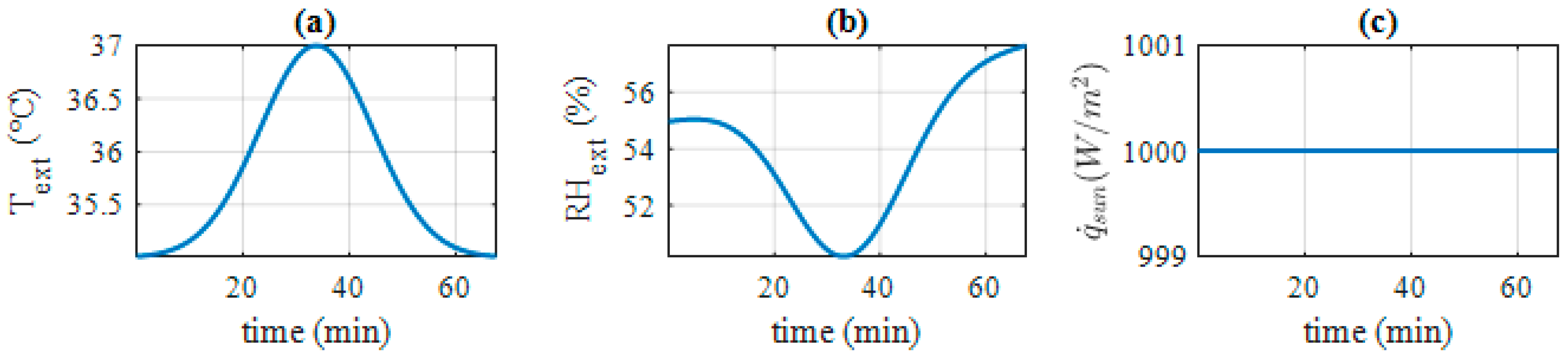
| Data | Values |
|---|---|
| External temperature | |
| External relative humidity | |
| Solar irradiance | |
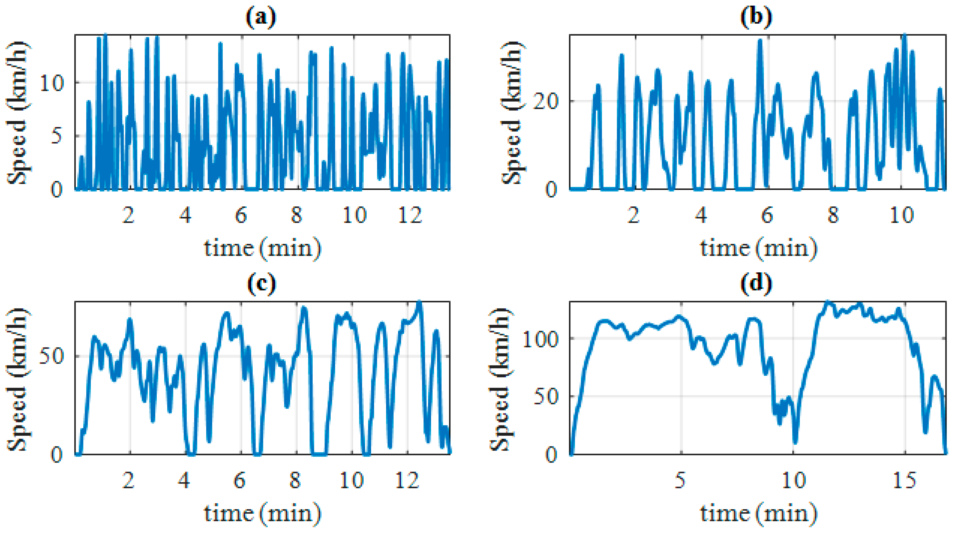
| Driving cycles | INRETS A2, R2, UF1, UL1 |
| Driver’s clothing | Formal and informal clothing |
| Vehicle | Small size electric vehicle |
| Electric motor power | 60 kW |
| Battery capacity | 40 kWh |
| Clothing | |||
|---|---|---|---|
| Informal | 0 | 28.3 | 28.0 |
| 500 | 34.2 | 26.2 | |
| 1000 | 40.0 | 24.1 | |
| Formal | 0 | 26.4 | 26.1 |
| 500 | 32.2 | 24.2 | |
| 1000 | 38.0 | 22.1 |
© 2020 by the authors. Licensee MDPI, Basel, Switzerland. This article is an open access article distributed under the terms and conditions of the Creative Commons Attribution (CC BY) license (http://creativecommons.org/licenses/by/4.0/).
Share and Cite
Lahlou, A.; Ossart, F.; Boudard, E.; Roy, F.; Bakhouya, M. Optimal Management of Thermal Comfort and Driving Range in Electric Vehicles. Energies 2020, 13, 4471. https://doi.org/10.3390/en13174471
Lahlou A, Ossart F, Boudard E, Roy F, Bakhouya M. Optimal Management of Thermal Comfort and Driving Range in Electric Vehicles. Energies. 2020; 13(17):4471. https://doi.org/10.3390/en13174471
Chicago/Turabian StyleLahlou, Anas, Florence Ossart, Emmanuel Boudard, Francis Roy, and Mohamed Bakhouya. 2020. "Optimal Management of Thermal Comfort and Driving Range in Electric Vehicles" Energies 13, no. 17: 4471. https://doi.org/10.3390/en13174471
APA StyleLahlou, A., Ossart, F., Boudard, E., Roy, F., & Bakhouya, M. (2020). Optimal Management of Thermal Comfort and Driving Range in Electric Vehicles. Energies, 13(17), 4471. https://doi.org/10.3390/en13174471