Abstract
Modular multilevel converters (MMCs) play an important role in the power electronics industry due to their many advantages, such as modularity and reliability. In the current research, the simulation method is used to study the system. However, with the increasing number of sub-modules (SMs), it is difficult to model and simulate the system. In order to overcome these difficulties, this paper presents a universal mathematical model (UMM) of MMC using half-bridge cells as SMs. The UMM is a full-scale model with switching state, capacitance, inductance, and resistance characteristics. This method can calculate any number of SMs, and it does not need to build a simulation model (SIM) of physical MMC—in particular, parametric design can be realized. Compared with the SIM, the accuracy of the proposed UMM is verified, and the computational efficiency of the UMM is 8.7 times higher than the simulation method. Finally, by utilizing the proposed UMM method, the influence of the parameters of MMCs is studied, including the arm induction, SM capacitance, SM number, and output current/voltage total harmonic distortion (THD) based on the UMM in the paper. The results offer an engineering insight to optimize the design of MMCs.
1. Introduction
With the rapid development of offshore wind farms, the demand for a high power, high-quality transmission system becomes more urgent. Modular multilevel converter (MMC)-based high voltage direct voltage (HVDC) technology provides a promising solution, due to its advantages of modularization, scalability, high efficiency, excellent harmonic performance, fault blocking ability, small filter size, high efficiency, and low redundancy cost [1,2,3]. MMC has been applied to many industries, such as energy storage systems, medium-voltage and high-power motor drive systems, distribution systems, etc. [4,5,6,7,8].
However, it is difficult to formulate an explicit expression of MMC, because it is a hybrid system of discrete and continuous models. The main feature of MMCs is the cascaded connection of a large number of sub-modules (SMs). These SMs are arranged in groups called arms or branches. The low-frequency voltage or current at the AC side is controlled by high-frequency switching values to manage SMs on/off. Therefore, the interaction between the arm and line quantities (variables) generates low- and high-frequency components on the AC and DC side of the SMs in an MMC [9]. In other words, MMC has strong coupling nonlinear multi-input and multi-output dynamic features [10]. The simulation studies were utilized to analyze the behavior of an MMC. However, the simulation process consumes time and computer resources to create a large number of SMs (up to 400 per arm) [11]. For example, a traditional detailed model (TDM) of MMC requires hundreds and thousands of Insulated Gate Bipolar Transistors(IGBTs) with antiparallel diodes and capacitors to be built and electrically connected in the simulation package’s graphical user interface, resulting in a large admittance matrix.
To simplify the simulation model, the conventional switching models/detailed models with full capabilities of replicating the conduction of power electronic devices such as IGBTs and their anti-parallel diodes are inefficient for the modeling of MMC-HVDC, as the simulation time is prohibitively long [1]. To simplify the calculation, it was assumed that the SM capacitor voltages are well balanced at their reference values [12,13]. The SM terminal voltage in each arm was modeled as a single equivalent voltage source [14]. In [15], the equivalent model was used and a small-signal analysis was carried out. Alternatively, each arm of MMC was modeled as a nonlinear capacitor with a time-variant sinusoidal capacitance [16]. Moreover, to simplify the analysis, the average value models (AVMs) are presented in [17,18,19,20]. However, the methods above do not reflect the switching state and the transient process of the SM capacitor voltage.
To address this problem, an efficient model was proposed by Udana and Gole in [21], which is referred to as the detailed equivalent model (DEM) in this paper; yet, a drawback of the DEM is that the individual converter components are invisible to the user. A new model, referred to as the accelerated model (AM), was proposed by Xu et al. in [22], but a full and objective comparison could not be completed because different researchers built the models on different computers. In [23], an enhanced accelerated model (EAM) with improved simulation speed was proposed by Antony et al., which further improved the computational efficiency of one method. A new dynamic phasor (DP) model of an MMC with an extended frequency range for direct interfacing with an electromagnetic transient (EMT) simulator was presented in [24]. In reference [25], a method of MMC modeling and design based on parametric and model-form uncertainty quantification is proposed, which can establish confidence in modeling and simulation in the presence of manufacturing variability and modeling errors, and may eliminate the need for heuristic safety factors. However, the high-efficiency calculation of large-scale SMs is not involved. The internal dynamics of the MMC are modeled considering the dominant harmonic components of each variable. However, the improved simulation models introduced above are based on Power Systems Computer Aided Design/Electromagnetic Transients including DC(PSCAD/EMTDC) for electromagnetic transient simulation. It is inconvenient to set variable parameters or change the topology of the whole circuit. It cannot be satisfied by loop calculation to compare the changes of parameters.
In this paper, a universal mathematical model for MMC is proposed which can reflect the steady-state and dynamic process of MMC. The model is a detailed numerical model, including the capacitor voltage and switch function of SMs. It can be implemented by a computer for any number of SMs. The whole model is parametric programmed; by setting one or several parameters, the desired results can be quickly obtained. Compared with the simulation model, this algorithm can easily modify the circuit parameters by setting cycle statements, and automatically carry out repeated simulation and multi-state simulation, so it is convenient to observe the operation characteristics of the system under different parameter values. Using the proposed MMC, the output voltage and the current THDs of MMC have been analyzed under different parameters (such as module number, capacitor voltage, arm inductance). In addition, the change in the capacitance voltage has been studied as one capacitance value decayed.
Without losing generality, in this paper the research is based on MATLAB/Simulink because of its powerful numerical calculation ability and rich processing module (such as Pulse Width Modulation (PWM) generator, and various transformation and comparison modules), especially the demonstration of control strategy. Compared with Simulink, PLECS is more professional, but does not have as many toolboxes as Simulink. The LTSpice installation package is small, easy to operate, and fast, but most of the support is for the ADI company’s own chip model. PSIM has the advantages of simple operation and fast simulation speed, and supports mainstream simulation mode analysis. However, due to the use of ideal switches, the simulation accuracy is limited.
This paper is organized as follows. Section 2 introduces the MMC topology, operation, and mathematical model. The algorithm of the universal mathematical model (UMM) is explained in Section 3. The correctness of the UMM is demonstrated in Section 4. A performance analysis under different conditions is shown in Section 5. The conclusions of the study are presented in Section 4.
2. Topology and Mathematical Model of the MMC
Topology and Principles of Operation
The circuit structure of a three-phase MMC is shown in Figure 1. The single-phase consists of an upper and a lower arm. Each arm is composed of N sub-modules (SM), and an inductor and equivalent resistance are connected in series. Each individual SM contains a capacitor and two complementary insulated gate bipolar transistor modules (i.e., and ). In this paper, the subscript means three-phase; , where represents the upper arm and represents a lower arm; represents the number of sub-modules. The rest of the symbols are as follows: (the arm inductance), (the arm equivalent resistance), (the arm voltage), (the arm current), (the AC side voltage), (the output current), (the circulating current), (the load inductance), (the load resistance), (the DC source voltage), (the capacitor voltage).
where is the switch function of the nth SM in the arm of phase-j, and its value is 1 or 0; is the SM capacitance.
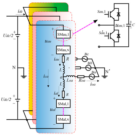
Figure 1.
Structure of a three-phase MMC-based inverter and its SM.
The relationship between the arm voltage and the capacitor voltage in phase-j and the switching function is:
Considering a fictitious midpoint in the DC side of Figure 1 and using Kirchhoff’s circuit laws, the following mathematical equations that govern the dynamic behavior of the MMC in phase-j can be obtained:
The arm currents can be expressed as:
where is the circulating currents flowing through phase-j of the MMC and can be calculated by Equation (7):
Substitute (3) and (5) into (4), and the dynamics of phase-j AC-side currents can be obtained as:
Similarly, the dynamic behavior of the circulating current in phase-j can be obtained by substituting (3) and (7) into (4):
Based on (1), (2), (8), and (9), the state-space equation of the MMC in phase-j can be described as:
where is the state vector is a perturbation vector; the desired value ( of is presented in Equation (11); is a time-varying structure state matrix, presented in (12); and is the perturbation coefficient matrix, presented in (20).
where is the voltage effective value (RMS) on the AC side, is the AC system frequency, and is the initial phase angle in phase-j.
where is a constant matrix in (13), and and are time-varying matrixes in (14) and (18), respectively.
where ; is presented in (15); is presented in (16); and is the input control vector, presented in (17).
where is as follows:
where is as follows:
The output voltage of the MMC, such as phase-j, is defined as the voltage difference from point j to N.
In (10), the control of the system is to adjust the structure of matrix so that , (or the active power and reactive power are close to their desired values). As the focus of the paper is the universal mathematical model of the controlled object, the control method is shown in reference [26], and will not be detailed here.
From Equation (8), we can get the formula of as follows (in active inverter, , = 0; in passive inverter, ,0):
3. Algorithm of the Universal Mathematical Model
Equation (10) shows that the MMC is a nonlinear multi input system where the nonlinearity consists of the products between the states and inputs. The direct solution is difficult to find; as a result, the discrete sampling method will be used. The algorithm of the universal model is shown in Figure 2.
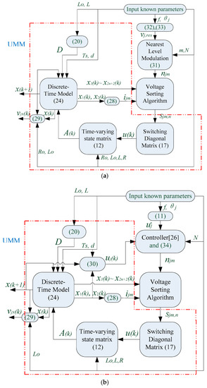
Figure 2.
Block diagram of the universal mathematical model algorithm for MMC. (a) Open-loop control system, (b) closed-loop control system.
3.1. Discrete-Time Model of the MMC
It is assumed that the switching of equations occurs at the sampling points. Based on (10) and assuming a sampling time of , the discrete-time model of the MMC, based on a forward Euler approximation, is obtained as:
The output current, , can be calculated as:
The circulating current, , is obtained by Equation (26):
The capacitance voltage,, is obtained by the following Equation:
Based on Equations (6), (25), and (26), the arm currents can be calculated as:
Based on Equation (22), the output voltage of the MMC can be expressed as:
Based on Equation (23), the AC voltage of the MMC can be expressed as:
3.2. Nearest Level Modulation
The nearest level modulation (NLM), also known as the round method, is an approach that uses the nearest voltage level to estimate the desired output voltage. The three phases are controlled independently. Given a normalized voltage reference , the nearest output voltage level can be determined by:
where is the modulation coefficient, and is defined as:
where is the initial phase angle in phase-j. Normalized voltage references for the three phases can be presented as:
3.3. Control Systems
In this paper, the control strategy applied in [26] is utilized to obtain the optimal value and through the tracking control of the AC voltage or DC voltage. Of course, not limited to this control strategy, other controls (such as the traditional PI control) are also applicable.
where is the capacitor-rated voltage, .
The MMC control diagram is shown in Figure 3, and a more detailed closed-loop control is shown in Figure 2b. Since this study focuses on the universality of the model controlled (UMM), only the system is considered as an open-loop system (in Figure 2a) in the early stage of the design, and the control system is designed after the system-controlled parameters are fixed.

Figure 3.
MMC control diagram.
3.4. Voltage Sorting Algorithm
In this paper, the voltage sorting algorithm applied in [27] is utilized to equalize all the capacitor voltages of the MMC . The algorithm reads the insertion indices and and determines which SMs are connected or bypassed in each arm of the MMC according to the plus-minus of the arm current . For example, if > 0, the algorithm connects SMs with the lowest voltages in the corresponding arm and bypasses all the others. Conversely, if < 0, the algorithm connects SMs with the highest voltages and bypasses the others. Therefore, the switching signals to be applied in the sampling time can be obtained. Finally, is obtained based on (17).
4. Verification of Universal Mathematical Model
To evaluate the performance of the proposed UMM, a comparison between the results from the UMM and the nonlinear time-domain simulation model has been conducted. The nonlinear time-domain simulation model (SIM) is implemented in MATLAB/Simulink, and the UMM is performed using an m-file in MATLAB. The initial value is set as . The comparison was conducted for a single-phase converter with 20 submodules. The main parameters of the MMC in the simulation are listed in Table 1. All the simulations were conducted using a Microsoft Windows 10 operating system with a 2.7 GHz Intel® core ™ i7-7500U processor and 16 GB of RAM. The test results are given in the following sub-sections.

Table 1.
Main parameters of the MMC (phase-a).
4.1. Accuracy Analysis
The waveforms calculated by the UMM were compared with those generated from the SIM to evaluate the accuracy of the proposed approach. The results are shown in Figure 4 and Figure 5. In these figures, the solid line “I” represents the result of UMM, the dashed line “II” represents the result of SIM.

Figure 4.
Output current/voltage diagram of the MMC. “I” represents the result of UMM, “II” represents the result of SIM. (a) current , (b) voltage .
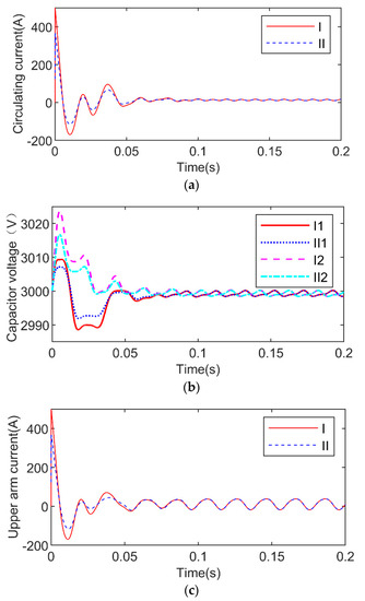
Figure 5.
Circulating current/capacitor voltage diagram of the MMC. “I” represents the result of UMM, “II” represents the result of SIM. (a) circulating current , (b) voltage . “1” represents the upper arm, “2” represents the lower arm, (c) upper arm current .
4.1.1. Dynamic Simulation under Normal Operation
Figure 4 displays the out current, , and output voltage, , versus time. It shows that within a 0.2 s time range, the results calculated via UMM are favorable compared with the result obtained from SIM. According to Table 2, the root mean square errors are within a reasonable range. These results demonstrate the accuracy of the UMM method at steady state.
Table 2.
Root mean square error of UMM and SIM.
For example, Figure 5a shows the transient behaviors of the circulating current. Figure 5b shows a trend of capacitor voltages for the upper and lower arm from transient to steady state. The upper arm current waveform is shown in Figure 5c. Before 0.06 s, the system was at a transient state, and the UMM and SIM results had shown similar behavior with a slight amplitude difference. After the transient state, the system tended to be stable and the two results were completely coincident.
The root mean square errors are shown in Table 2. From the numerical point of view, except for the errors of other variables are small. In the meantime, the value of is only less than 3/10,000 relative to its RMS (21,216 V).
In short, the perfect coincidence of the above-mentioned various dynamic waveforms (output current /voltage , circulating current , capacitive voltage , and upper arm current ) has proved the accuracy and correctness of the proposed algorithm UMM.
4.1.2. Dynamic Simulation of SM Open Circuit Fault
The open circuit fault of SM was assumed to study the effect of the internal fault of sub module on the MMC system. The time interval of failure is given as [3, 3.04]—i.e., two cycles.
In Figure 6, it can be seen that in the transient process of fault, the waveforms of UMM and that of SIM also match well.

Figure 6.
The waveform in case of open circuit fault. “I” represents the result of UMM, “II” represents the result of SIM. (a) output voltage, (b) circulating current, (c) capacitor voltage waveform in the case of open circuit fault.
4.2. Computational Efficiency
A 5 s period was tested with a 50 µs simulation time step. In this paper, we considered three groups of data (number of submodules, N = 8, 12, 20) for calculation, and the calculation results are shown in Figure 7. For example, when N = 20, the UMM took 7.1 s to get the result, while SIM consumed 62.2 s. The computational efficiency of UMM is significantly improved, which is about 8.7 times faster than that of SIM. However, the computational efficiency of the average value model (AVM) lies in the middle of the three.

Figure 7.
CPU times for UMM and SIM.
Another advantage of UMM over SIM is that the SIM system took a large amount of time to build a system with many SMs.
Under different sampling times (10, 30, 50 µs), the Central Processing Unit (CPU) times for UMM have been shown in Figure 8 as a 0.1 s period. It can be seen in Figure 8 that at N < 150, the three sampling times have little difference. However, with the increase in N, the time gap among them becomes larger. Especially when N is 404, the CPU times of the three were 162.8, 44.0, and 25.5 s, respectively. However, in fact, only the sampling time 50 µs for the UMM system met the accuracy requirements.

Figure 8.
CPU times for UMM under different sampling times.
5. Application Based on UMM
Section 4 had proved the accuracy and efficiency of UMM. However, in this section, UMM will be used to study the MMC system, which is also the biggest difference from most existing models. The quality of the output voltage and current is a criterion to judge the performance of an inverter. For a long time, it was believed that the output current and voltage quality would be improved with an increase in the SM quantity, but there is no definite conclusion and mathematical evidence for this.
It is time-consuming to build simulation models, so it is impossible to simulate and analyze a large number of SMs. The utilization of UMM can facilitate this analysis. In this section, the influence of the number N of SMs on the output voltage and current THD under different conditions will be investigated. The dynamic performance of the MMC system was analyzed on the effects of different Ns.
5.1. Output Voltage/Current Harmonic Performance under Different N Values
The calculation parameters are given with Table 1, except for the parameter N, where N is an independent variable from 0 to 400. The simulation results are shown in Figure 9.

Figure 9.
The oscillogram varying with the number of SM. (a) Output voltage THD, (b) output voltage fundamental amplitude, (c) output current THD, (d) output current fundamental amplitude.
In Figure 9, during the period when N was increased from 4 to 50, both the THD and fundamental amplitude decreased rapidly. After that, as N increased, the change rate tends to reduce. The optimal value was at (308, 0.352%) in Figure 9a, and (92, 0.1335%) in Figure 9c. The fundamental amplitude reached the minimum value at N = 28, then increased slightly in Figure 9b,d. After N > 50, it reached a stable state with small fluctuations.
In summary, the results show that the relationship between the quality of output voltage (or current) and the number N of SMs is not proportional. It has an optimal solution; using UMM, it is possible to find the optimal solution. In practice, in the design of N should be also considered the cost of hardware, the voltage grade, and the complexity of control.
5.2. Output Voltage/Current Harmonic Performance under Different SM Capacitance and N Values
The influence of different SM capacitances, C, is studied in this section. The results are shown in Figure 10.

Figure 10.
The THD diagram of the output current varying with and N. The value is shown in the legend.
Figure 10 displays the THD value of the output current and voltage changing with a different number N of SMs and SM capacitance , respectively. As illustrated, when the N is small, less than 50, the THD basically coincides with different C values. After N > 100, the THD of the curve of C = 0.5 mF rises rapidly and become unstable. This phenomenon indicates that, along with the increase in the SMs, the capacity should be increased accordingly to keep the system stable.
According to [28], the voltage fluctuation rate of the SM capacitor can be calculated in the following equation:
where is the MMC nominal power, and .
Substitute into (32), then:
Generally, ,, and are constants. As a result, is directly proportional to N and inversely proportional to C. When N increases and C is a fixed value, the system will diverge and become unstable after exceeds the allowable value.
5.3. Output Voltage/Current Harmonic Performance under Different Arm Inductance and N Values
The influence of different SM inductances, L, is studied in this section. The simulation results are shown in Figure 11.
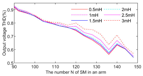
Figure 11.
The THD diagram of the output voltage varying with and N. The L value is shown in the legend.
In Figure 11, when N is less than 110, the THD of the output voltage is basically the same for all the inductance values; after that, the THD decreases slowly as N increases, but the larger the arm inductance value, the higher the THD. It shows a small mutation near N = 140.
Figure 12 shows the THD value of the output voltage changing with N and . When N is less than 40, the output current THD is around the same value. The inductance value has different effects on THD in different areas of N. For example, the areas with the smallest THD are as follows: = 1 mF, N [44, 56]; = 1.5 mF, ; = 3 mF in the interval [68, 80], = 0.5 mF, in the interval [68, 100]. After N increased to greater than 96, the THD increases significantly with the increase in L.

Figure 12.
The THD diagram of the output current varying with and N.
From the general trend, as N becomes larger, the inductance value should become smaller. However, if the inductance value is too small, it will lose the effect of suppressing the arm current and fault tolerance. Therefore, the design should be selected based on the actual situation.
5.4. Dynamic Performance under SM Capacitance Decay Fault
In this test, the capacitance of the was attenuated by 0.6 times. Shown as Figure 13, the failure occurred at 3 s and continued until the end. From the SM voltage waveform, the difference between the waveforms before and after 3 s is obvious. This means that, in addition to the IGBT open circuit fault mentioned above, the proposed model can also study the parameter fault.

Figure 13.
The SM1 capacitor voltage diagram under capacitance decay fault.
5.5. Object-Oriented Parametric Design
Through object-oriented programming in Figure 14, the program can realize human-computer interaction and reduce the workload of designers, so as to realize the universality, versatility, ease of use, and operation of MMC. Of course, this is only an example. See reference [28] for the calculation of relevant parameters, which will not be discussed here.

Figure 14.
Design and verification interface for MMC.
6. Conclusions
A general mathematical model has been derived in detail from the circuit structure of MMC in this paper. The mathematical model includes the non-linear or linear characteristics of switching state, capacitance voltage, inductance, and resistance. Compared with the traditional MATLAB/Simulink (21-level MMC), the output voltage/current, circulating current, and capacitor voltage coincide, and the accuracy of the proposed model is fully proved. Additionally, this model is 8.7 (N = 20) times faster than the traditional simulation method. By changing the arm induction, SM capacitance, and the number of SMs to study the impact of each parameter on the output current/voltage THD, the optimal number of SMs has been found. In addition, the proposed model can also analyze the structure and parameter faults of MMC. The UMM proposed lays a solid foundation for further research into the dynamic performances of MMC with a large number of SMs.
The UMM mainly analyzes the static/dynamic system by discretizing the state equation of MMC. In essence, it belongs to the analytical analysis mathematical model. Its iterative calculation speed is much faster than that of the simulation model. At the same time, it also reduces the modeling time of the large-scale component modules and improves the universality. This is the reason that although the simulation model compared is only based on MATLAB/Simulink, it is not lost generality.
Author Contributions
Conceptualization, M.L. and Z.L.; methodology, M.L.; software, M.L.; validation, M.L.; resources, X.Y.; data curation, X.Y.; writing—original draft preparation, M.L.; writing—review and editing, M.L.; project administration, X.Y.; funding acquisition, Z.L. All authors have read and agreed to the published version of the manuscript.
Funding
This research was funded by the National Natural Science Foundation of China (No. 61963009) and (No. 61861007); Science and Technology Planning Project of Guizhou Province (No.2154 (2019)) and (No. 2302 (2016)); Collaborative Foundation of Guizhou Province (No. 7228 (2017)); Platform Talent Project of Guizhou Province (No. 5788 (2017)); and the special fund project of provincial governor for outstanding science and technology education talents in Guizhou Province (No. 4 (2010)).
Conflicts of Interest
The authors declare no conflict of interest.
Abbreviations
| MMC | modular multilevel converter |
| THD | total harmonic distortion |
| UMM | universal mathematical model |
| SIM | simulation model |
| NLM | nearest level modulation |
| TDM | traditional detailed model |
| AM | accelerated model |
| DP | dynamic phasor |
| HVDC | High-voltage direct voltage |
| SM | sub-module |
| DC | direct current |
| AC | alternating current |
| IGBT | insulated gate bipolar transistor |
| AVM | average value model |
| EAM | enhanced accelerated model |
| EMT | electromagnetic transient |
References
- Raju, M.N.; Sreedevi, J.; Mandi, R.P.; Meera, K.S. Modular multilevel converters technology: A comprehensive study on its topologies, modelling, control and applications. IET Power Electron. 2019, 12, 149–169. [Google Scholar] [CrossRef]
- Kouro, S.; Malinowski, M.; Gopakumar, K.; Pou, J.; Franquelo, L.G.; Wu, B.; Rodriguez, J.; Perez, M.A.; Leon, J.I. Recent advances and industrial applications of multilevel converters. IEEE Trans. Ind. Electron. 2010, 57, 2553–2580. [Google Scholar] [CrossRef]
- Debnath, S.; Member, S.; Qin, J.; Member, S.; Bahrani, B. Operation, Control, and Applications of the Modular Multilevel Converter: A Review. IEEE Trans. Power Electron. 2015, 30, 37–53. [Google Scholar] [CrossRef]
- Nguyen, T.H.; Al Hosani, K.; El Moursi, M.S.; Blaabjerg, F. An Overview of Modular Multilevel Converters in HVDC Transmission Systems with STATCOM Operation during Pole-to-Pole DC Short Circuits. IEEE Trans. Power Electron. 2019, 34, 4137–4160. [Google Scholar] [CrossRef]
- Picas, R.; Zaragoza, J.; Pou, J.; Ceballos, S.; Konstantinou, G.; Capella, G.J. Study and comparison of discontinuous modulation for modular multilevel converters in motor drive applications. IEEE Trans. Ind. Electron. 2019, 66, 2376–2386. [Google Scholar] [CrossRef]
- Li, B.; Zhou, S.; Xu, D.; Yang, R.; Xu, D.; Buccella, C.; Cecati, C. An Improved Circulating Current Injection Method for Modular Multilevel Converters in Variable-Speed Drives. IEEE Trans. Ind. Electron. 2016, 63, 7215–7225. [Google Scholar] [CrossRef]
- Perez, M.A.; Bernet, S.; Rodriguez, J.; Kouro, S.; Lizana, R. Circuit topologies, modeling, control schemes, and applications of modular multilevel converters. IEEE Trans. Power Electron. 2015, 30, 4–17. [Google Scholar] [CrossRef]
- Li, J.; Konstantinou, G.; Member, S.; Wickramasinghe, H.R.; Member, S.; Pou, J. Operation and Control Methods of Modular Multilevel Converters in Unbalanced AC Grids: A Review. IEEE J. Emerg. Sel. Top. Power Electron. 2019, 7, 1258–1271. [Google Scholar] [CrossRef]
- Ilves, K.; Antonopoulos, A.; Norrga, S.; Nee, H.-P. Steady-state analysis of interaction between harmonic components of arm and line quantities of modular multilevel converters. IEEE Trans. Power Electron. 2012, 27, 57–68. [Google Scholar] [CrossRef]
- Vatani, M.; Member, S.; Hovd, M.; Member, S. Control of the Modular Multilevel Converter Based on a Discrete-Time Bilinear Model Using the Sum of Squares Decomposition Method. IEEE Trans. Power Del. 2015, 30, 2179–2188. [Google Scholar]
- Dekka, A.; Wu, B.; Fuentes, R.; Perez, M.; Zargari, N. Evolution of Topologies, Modeling, Control Schemes, and Applications of Modular Multilevel Converters. IEEE J. Emerg. Sel. Top. Power Electron. 2017, 5, 1631–1656. [Google Scholar] [CrossRef]
- Vatani, M.; Member, S.; Bahrani, B. Indirect Finite Control Set Model Predictive Control of Modular Multilevel Converters. IEEE Trans. Smart Grid 2015, 6, 1520–1529. [Google Scholar] [CrossRef]
- Wang, J.; Liang, J.; Gao, F.; Xiaoming, D.; Wang, C.; Zhao, B. A Closed-Loop Time-Domain Analysis Method for Modular Multilevel Converter. IEEE Trans. Power Electron. 2017, 32, 7494–7508. [Google Scholar] [CrossRef]
- Saad, H.; Peralta, J.; Dennetiere, S.; Mahseredjian, J.; Jatskevich, J.; Martinez, J.A.; Davoudi, A.; Saeedifard, M.; Sood, V.; Wang, X. Dynamic averaged and simplified models for MMC based HVDC transmission systems. IEEE Trans. Power Del. 2013, 28, 1723–1730. [Google Scholar]
- Leon, A.E.; Amodeo, S.J. Modeling, control, and reduced-order representation of modular multilevel converters. Electr. Power Syst. Res. 2018, 163, 196–210. [Google Scholar] [CrossRef]
- Belhaouane, M.M.; Ayari, M.; Guillaud, X.; Braiek, N.B. Robust Control Design of MMC-HVDC Systems Using Multivariable Optimal Guaranteed. IEEE Trans. Ind. Appl. 2019, 55, 2952–2963. [Google Scholar] [CrossRef]
- Xu, J.; Gole, A.M.; Zhao, C. The use of averaged-value model of modular multilevel converter in DC grid. IEEE Trans. Power Del. 2015, 30, 519–528. [Google Scholar]
- Meng, X.; Han, J.; Bieber, L.; Wang, L.; Li, W.; Belanger, J. A Universal Blocking-Module-Based Average Value Model of Modular Multilevel Converters with Different Types of Submodules. IEEE Trans. Energy Convers. 2020, 35, 53–66. [Google Scholar] [CrossRef]
- Lyu, J.; Zhang, X.; Cai, X.; Molinas, M. Harmonic State-Space Based Small-Signal Impedance Modeling of a Modular Multilevel Converter with Consideration of Internal Harmonic Dynamics. IEEE Trans. Power Electron. 2019, 34, 2134–2148. [Google Scholar] [CrossRef]
- Freitas, C.M.; Watanabe, E.H.; Monterio, L.F.C. A linearized small-signal Thévenin-equivalent model of a voltage-controlled modular multilevel converter. Electr. Power Syst. Res. 2020, 182, 106231–106241. [Google Scholar] [CrossRef]
- Gnanarathna, U.N.; Gole, A.M.; Jayasinghe, R.P. Efficient modeling of modular multilevel HVDC converters (MMC) on electromagnetic transient simulation programs. IEEE Trans. Power Del. 2011, 26, 316–324. [Google Scholar]
- Xu, J.; Zhao, C.; Liu, W.; Guo, C. Accelerated model of modular multilevel converters in PSCAD/EMTDC. IEEE Trans. Power Del. 2013, 28, 129–136. [Google Scholar]
- Beddard, A.; Barnes, M.; Preece, R. Comparison of Detailed Modeling Techniques for MMC Employed on VSC-HVDC Schemes. IEEE Trans. Power Deliv. 2015, 30, 579–589. [Google Scholar]
- Rupasinghe, J.; Member, S.; Filizadeh, S.; Member, S. A Dynamic Phasor Model of an MMC with Extended Frequency Range for EMT Simulations. IEEE J. Emerg. Sel. Top. Power Electron. 2019, 7, 30–40. [Google Scholar] [CrossRef]
- Rashidi, N.; Burgos, R.; Roy, C.; Boroyevich, D. On the Modeling and Design of Modular Multilevel Converters with Parametric and Model-Form Uncertainty Quantification. IEEE Trans. Power Electron. 2020, 35, 10168–10179. [Google Scholar] [CrossRef]
- Liu, M.; Li, Z.; Yang, X. Tracking Control of Modular Multilevel Converter Based on Linear Matrix Inequality without Coordinate Transformation. Energies 2020, 13, 1978. [Google Scholar] [CrossRef]
- Gutierrez, B. Modular Multilevel Converters (MMCs) Controlled by Model Predictive Control with Reduced Calculation Burden. IEEE Trans. Power Electron. 2018, 33, 9176–9187. [Google Scholar] [CrossRef]
- Zheng, X. HVDC System, 2nd ed.; China Machine Press: Beijing, China, 2016; pp. 69–71. [Google Scholar]


© 2020 by the authors. Licensee MDPI, Basel, Switzerland. This article is an open access article distributed under the terms and conditions of the Creative Commons Attribution (CC BY) license (http://creativecommons.org/licenses/by/4.0/).