Analysis of Unified Power Flow Controller Steady-State Power Flow Regulation Capability and Its Key Factors

Abstract

As the latest generation of flexible AC transmission system (FACTS) devices, the unified power flow controller (UPFC) has comprehensive control capability and has played an important role in modern power systems. Research on UPFC steady-state power flow regulation capability is valuable for the design and operation of UPFC projects. To analyze the UPFC regulation capability, in this paper, the interaction between the UPFC and the external system is studied and the key factors of UPFC regulation capability are analyzed. It is demonstrated that the changes in the voltage magnitude and phase angle difference of UPFC-embedded line terminals will hinder the UPFC from regulating the power flow and decrease the UPFC regulation capability. Therefore, the UPFC power flow regulation capability is not only related to the parameters of the UPFC and its installation line, but also related to grid parameters. To analyze the UPFC active power flow regulation capability in practical power grids, the relationship between the UPFC regulation capability and grid parameters is deduced, and an estimation method is proposed to calculate the regulation range. Then, the estimation method is applied in the Chuxiong Power Grid and compared with power flow calculations. The results verify the UPFC power flow regulation characteristics given by the analysis and the effectiveness of the estimation method. Besides, it is shown that the estimation method can lower the requirements for the power flow calculation program, and reduce computation load.

1. Introduction

A variety of flexible AC transmission system (FACTS) devices, including the thyristor controlled series capacitor (TCSC), thyristor controlled phase shifter (TCPS), static synchronous series compensator (SSSC), unified power flow controller (UPFC), etc., have the function of adjusting line power flows [1]. They provide an effective means to enhance the efficiency and security of power systems [2,3]. Among them, the UPFC has received extensive attention in recent years. Three UPFC projects have been put into operation in the past five years and have played an important role in power flow control, power transfer capability enhancement, and reactive power compensation [4,5]. The realization of the above UPFC functions is inseparable from the UPFC power flow regulation capability. Therefore, research on UPFC steady-state power flow regulation capability, especially the active power flow regulation capability, is valuable for the design and operation of UPFC projects.

The regulation capability has been studied since the proposal of the UPFC concept [6]. In [6], it is illustrated that the UPFC is capable of controlling all basic power system parameters which determine the power flow. In [7], it is shown that the UPFC is able to control the active power flow and reactive power flow of the transmission line, simultaneously or independently. Besides, the power flow control region of the UPFC-embedded line is presented, under the assumption that the ends of the line are connected to voltage sources (which means the voltage magnitudes and phase angles of the buses are constant). Under the same assumption, the calculation formulas of the UPFC-embedded line power flow are derived in [8,9], and the power flow ranges under different operating conditions are given by numerical calculation. A simple two-machine system containing the UPFC is studied in [10,11]. In [10], the relationship between the injected voltage of the series converter and the line power flow are presented, and it is concluded that when taking the receiving-end system voltage phase as the reference, the active power flow is only controlled by the q-axis injected voltage. Furthermore, in [11], it is pointed out that when the sending-end bus voltage phase is taken as the reference, the q-axis component of the series converter output voltage is the main factor of the line active power flow, and the d-axis component is the main factor of the line reactive power flow. Moreover, it is shown in [11] that the control region boundaries of the active power flow and reactive power flow in the PQ plane are a series of ellipses, which change with the voltage magnitude of the series converter.

The above literature investigates the power flow regulation capability of the UPFC in small power systems and assumes that the operating states of the external system (such as bus voltage magnitudes and phase angles) are unchanged under different UPFC output scenarios. However, for practical power grids, the change in UPFC output will affect the operating states of the system, and the change in system operating states will in turn affect the power flow regulation of the UPFC. Therefore, it is necessary to analyze the relationship between the UPFC output and the system states.

In order to analyze the impact of different UPFC output on the operating states of the system, the UPFC is substituted by current sources in [12,13,14]. In [12], the relationship between line loads and the commands of the UPFC series converter is deduced, and it is pointed out that line loads are mainly related to the active power command. In [13], the relationship between bus voltage magnitude and the commands of the UPFC series converter is deduced, and it is pointed out that the reactive power command can be used to adjust the voltage magnitudes of adjacent buses. Furthermore, the relationship between the capacity of the UPFC series converter and the regulation requirement of line overload control is presented in [14]. Besides, in [15], the voltage and power flow sensitivities with respect to voltage source converter-based FACTS controllers are studied in a large system, and two approaches are proposed for the sensitivity analysis. Considering that in some cases (such as studying the system transmission usage and power transfer capability), we are mainly concerned with the line active power flow, a DC-based injection model of the UPFC-embedded line is developed in [16], and the impact of the UPFC on bus voltage angles and line active power flows is studied using the proposed model [17]. The above articles present different theoretical methods for analyzing the impact of the UPFC on system operating states, but they have not studied the power flow regulation capability of the UPFC.

In the existing literature, the UPFC regulation capability in complex power grids is usually studied by power flow calculations. Various UPFC models and calculation methods are developed for power flow studies [18,19], which lays the foundation for the power flow calculation of power systems with the UPFC. In [20], the boundary diagram for the American Electric Power (AEP) UPFC capability is calculated. It is pointed out: in theory, the UPFC series converter could inject any level of voltage, up to a constant maximum, with an arbitrary phase angle, but in the actual system, the output voltage of the UPFC is subject to many practical constraints, such as limits on the converter currents and the real power exchanged between the converters. These constraints and the system conditions together determine the achievable operating region of the UPFC [21]. In [22], the power flow of the 1673-bus system containing the Marcy UPFC is calculated, and it is illustrated that the dispatch trace of the UPFC at its rated capacity is an elliptically shaped curve, which is almost independent of the reactive power injection of the UPFC shunt converter. In [23,24], the power flow control capability of the Nanjing Western Power Grid (NWPG) UPFC is studied, and it is demonstrated that the actual power flow control range obtained by the power flow calculation is much smaller than the theoretical value due to the change in the external network operating states.

In summary, the regulation capability of the UPFC has not been fully researched, especially in the theoretical research. Most of the existing literature only conducts theoretical analysis on ideal systems and cannot effectively analyze the power flow regulation capability of the UPFC in complex systems. Due to the lack of theoretical analysis, the UPFC regulation capability in practical power systems is mostly given by power flow calculations. This leads to two problems. On the one hand, it is cumbersome to give the regulation capability of the UPFC through power flow calculations, because it is necessary to repeatedly calculate the power flow under different UPFC output. On the other hand, it is difficult to analyze and explain the characteristics of the UPFC regulation capability in different networks.

In order to make up for the shortcomings of the existing theory, this paper studies the interaction between the UPFC and the external system and analyzes the key factors of UPFC regulation capability. The main contributions and findings of this paper include:

• The UPFC regulation capability under different system conditions is analyzed. It is shown that the changes in the voltage magnitude and phase angle difference of UPFC-embedded line terminals will hinder the UPFC from regulating the power flow and decrease the UPFC regulation capability. The decrease of the active power regulation capability is mainly affected by the change in the phase angle difference, while the decrease of the reactive power regulation capability is mainly affected by the change in the voltage magnitude.
• The influence of UPFC capacity constraints on the regulation capability is analyzed. It is shown that the constraints of the shunt converter capacity and the exchanged power between the converters may reduce the reactive power regulation range, while the rated current of the UPFC series converter may reduce both the active and reactive power regulation range.
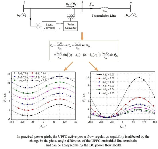
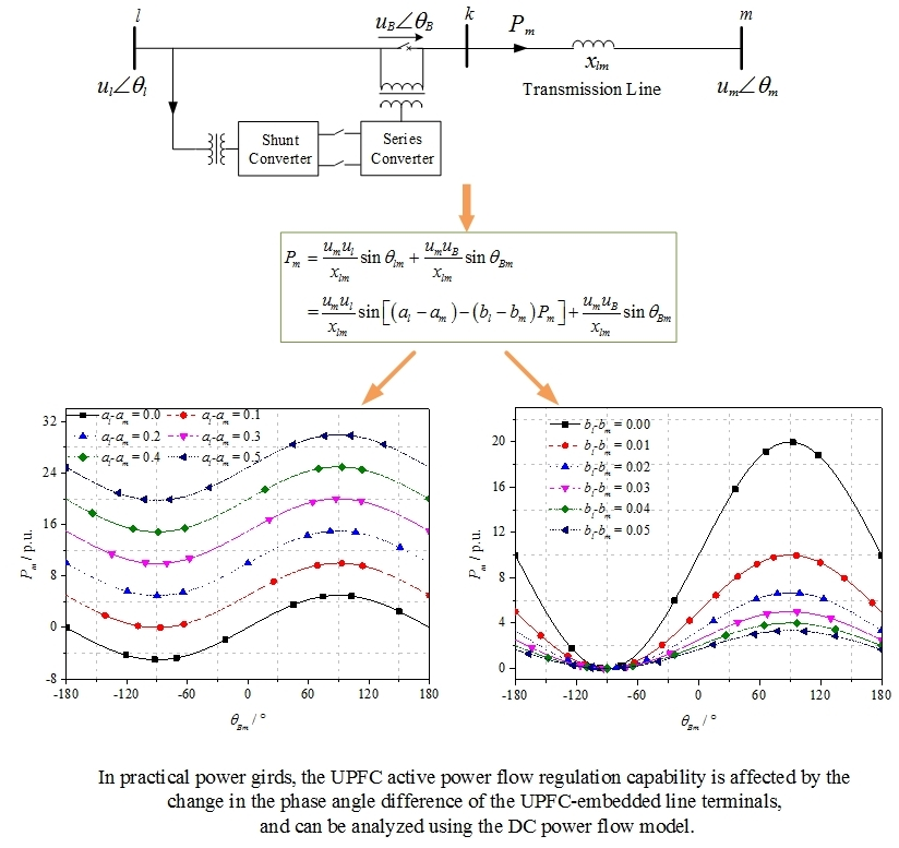
• The relationship between the UPFC active power flow regulation capability and grid parameters is deduced in complex power girds. Based on this relationship, the UPFC regulation characteristics under different grid parameters are presented, and an estimation method is proposed to calculate the active power flow regulation range.

The rest of this paper is organized as follows: The power flow regulation capability of the UPFC under ideal conditions is given in Section 2. The key factors of UPFC regulation capability are analyzed in Section 3. In Section 4, the relationship between the UPFC active power flow regulation capability and grid parameters is studied, and the estimation method is proposed. The correctness of the analysis results and the effectiveness of the proposed method are verified by power flow calculations in Section 5. At last, conclusions are drawn in Section 6.

2. Power Flow Regulation Capability of the UPFC under Ideal Conditions

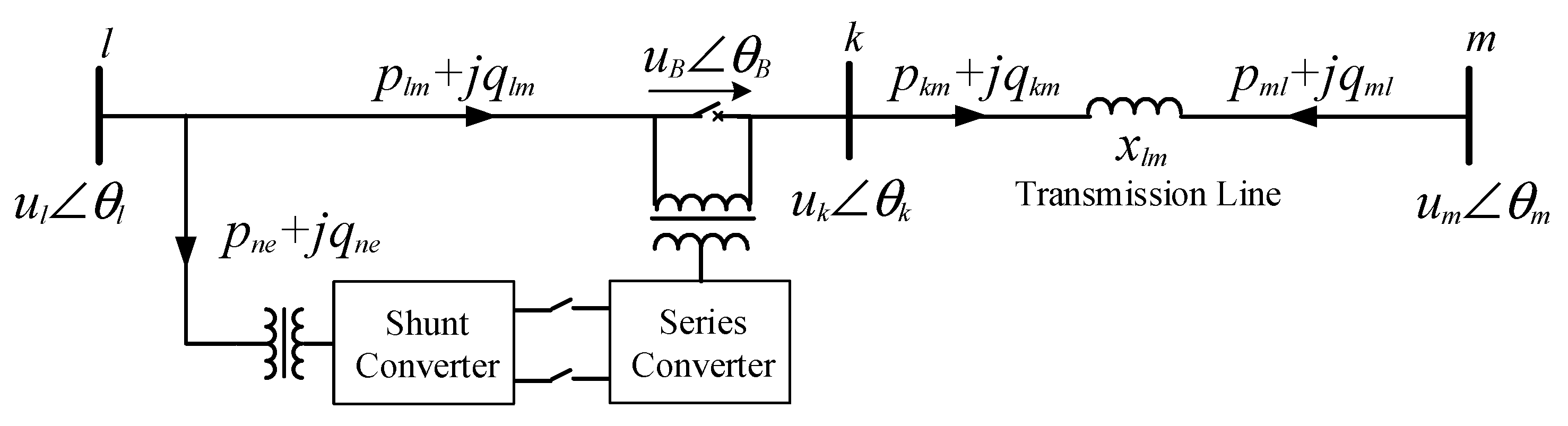
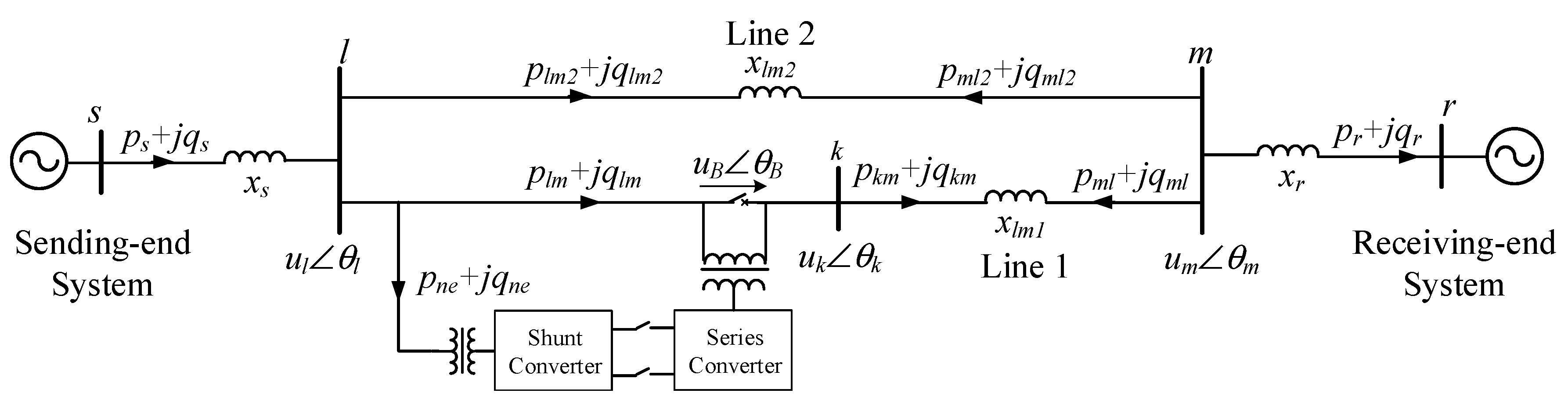
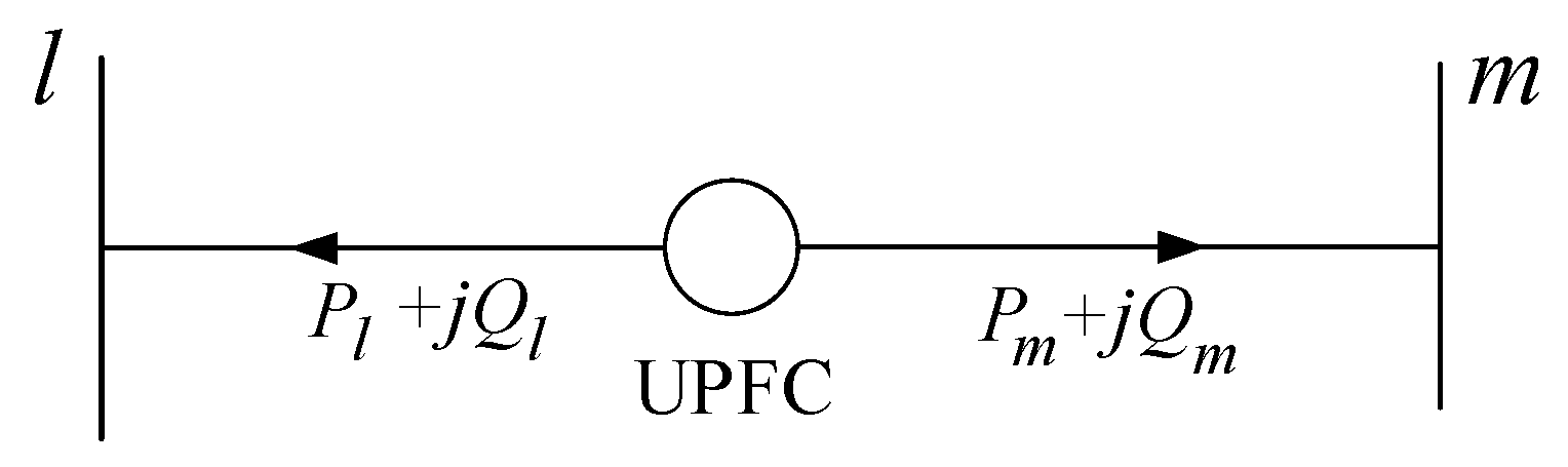
The UPFC-embedded line is shown in Figure 1. As shown in Figure 1, the UPFC is installed in line l-m. $u_l\angle {\theta }_l$, $u_k\angle {\theta }_k$, and $u_m\angle {\theta }_m$ are the voltages of bus l, bus k, and bus m. $u_B\angle {\theta }_B$ is the output voltage of the UPFC series converter. x_lm is the reactance of the transmission line. p_lm + jq_lm, p_ne + jq_ne, p_km + jq_km, and p_ml + jq_ml are the power flows of corresponding points.

The following ideal conditions are usually adopted in order to facilitate the analysis [7,8,9,10,11]:

(1)

When the power flow is regulated by the UPFC, the voltage magnitudes of the line terminals (i.e., u_l and u_m), are constant. Besides, the voltage phase angle difference between bus l and bus m are assumed to be unchanged, which means ${\theta }_l-{\theta }_m$ is constant.

(2)

The transmission line is equivalent to the reactance x_lm.

(3)

The losses of the UPFC are ignored.

According to the above conditions, the following conclusions can be drawn:

(1)

Since the power flow of the transmission line is only related to the parameters of the line, the bus voltages of both terminals, and the output of the UPFC, the influence of other lines in the system may be ignored, so only the UPFC-embedded line in Figure 1 is needed to be analyzed.

(2)

Since the voltage magnitude of the sending-end bus (bus l) is assumed to be constant, the reactive power exchanged between the shunt converter and the system has no effect on the bus voltage, and has no effect on the power flow of the transmission line.

(3)

Because the losses of the UPFC and the transmission line are both ignored, the active power flowing out of bus l is equal to that flowing into bus m.

Because the UPFC is mainly used to regulate the power flow of the transmission line to prevent line overload, the active power flow and the reactive power flow of the transmission line, which are p_km and q_km, are analyzed in this section. Taking the voltage phase angle of bus m as the reference phase, we have ${\theta }_{lm}={\theta }_l-{\theta }_m$, ${\theta }_{km}={\theta }_k-{\theta }_m$, and ${\theta }_{Bm}={\theta }_B-{\theta }_m$. Then according to Figure 1, p_km and q_km can be calculated as:

$$\{\begin{array}{l}{p}_{km}=\frac{u_m{u}_k}{x_{lm}}\sin {\theta }_{km}\\ q_{km}=\frac{u_k{}^2-u_m{u}_k\cos {\theta }_{km}}{x_{lm}}\end{array}$$

(1)

According to $u_k\angle {\theta }_{km}=u_l\angle {\theta }_{lm}+u_B\angle {\theta }_{Bm}$, we have:

$$\{\begin{array}{l}{u}_k\cos {\theta }_{km}=u_l\cos {\theta }_{lm}+u_B\cos {\theta }_{Bm}\\ u_k\sin {\theta }_{km}=u_l\sin {\theta }_{lm}+u_B\sin {\theta }_{Bm}\end{array}$$

(2)

According to Equation (2), Equation (1) can be written as:

$$\{\begin{array}{l}{p}_{km}=\frac{u_m{u}_l}{x_{lm}}\sin {\theta }_{lm}+\frac{u_m{u}_B}{x_{lm}}\sin {\theta }_{Bm}\\ q_{km}=\frac{u_l{}^2-u_m{u}_l\cos {\theta }_{lm}}{x_{lm}}+\frac{u_B{}^2-u_m{u}_B\cos {\theta }_{Bm}}{x_{lm}}+\frac{2u_l{u}_B\cos \left({\theta }_{lm}-{\theta }_{Bm}\right)}{x_{lm}}\end{array}$$

(3)

According to Equation (3), when the output voltage of the UPFC series converter is zero, the power flows of the transmission line are:

$$\{\begin{array}{l}{p}_{km0}=\frac{u_m{u}_l}{x_{lm}}\sin {\theta }_{lm}\\ q_{km0}=\frac{u_l{}^2-u_m{u}_l\cos {\theta }_{lm}}{x_{lm}}\end{array}$$

(4)

where p_km0 and q_km0 are the initial power flows of the uncompensated case.

When the output voltage of the UPFC series converter is not zero, the incremental active and reactive power flows, denoted by $\Delta p_{km}$ and $\Delta q_{km}$, with respect to p_km0 and q_km0 can be written as:

$$\{\begin{array}{l}\Delta p_{km}=\frac{u_m{u}_B}{x_{lm}}\sin {\theta }_{Bm}\\ \Delta q_{km}=\frac{u_B{}^2-u_m{u}_B\cos {\theta }_{Bm}}{x_{lm}}+\frac{2u_l{u}_B\cos \left({\theta }_{lm}-{\theta }_{Bm}\right)}{x_{lm}}\end{array}$$

(5)

According to Equation (5), the relationship between $\Delta p_{km}$ and $\Delta q_{km}$ satisfies:

$$\{\begin{array}{cc}\left(\frac{k_3{}^2+k_4{}^2}{k_1{}^2}\right)\Delta p_{km}{}^2-\frac{2k_3}{k_1}\Delta p_{km}\Delta q_{km}+\Delta q_{km}{}^2+\frac{2k_2{k}_3}{k_1}\Delta p_{km}-2k_2\Delta q_{km}+\left(k_2{}^2-k_4{}^2\right)=0,& k_4\ne 0\hfill \\ \Delta q_{km}=\frac{k_3}{k_1}\Delta p_{km}+k_2,& k_4=0\hfill \end{array}$$

(6)

where:

$$\{\begin{array}{l}{k}_1=\frac{u_m{u}_B}{x_{lm}}>0\\ k_2=\frac{u_B{}^2}{x_{lm}}>0\\ k_3=\frac{2u_l{u}_B}{x_{lm}}\sin {\theta }_{lm}\\ k_4=\frac{u_B}{x_{lm}}\left(2u_l\cos {\theta }_{lm}-u_m\right)\end{array}$$

(7)

According to Equation (6), the steady-state power flow regulation characteristics of the UPFC are as follows:

(1)

For the special case where $k_4=0$, when u_B is constant and ${\theta }_{Bm}$ changes, the $\Delta p_{km}$-$\Delta q_{km}$ curve is a straight line in the PQ plane. Accordingly, the p_km-q_km curve is also a straight line.

According to Equations (5) and (6), for a specific u_B, the ranges of $\Delta p_{km}$ and $\Delta q_{km}$ changing with ${\theta }_{Bm}$ are:

$$\{\begin{array}{l}\Delta p_{km}\in \left[-\frac{u_m{u}_B}{x_{lm}},\frac{u_m{u}_B}{x_{lm}}\right]\\ \Delta q_{km}\in \left[\frac{\left(u_B-\sqrt{4u_l{}^2-u_m{}^2}\right)u_B}{x_{lm}},\frac{\left(u_B+\sqrt{4u_l{}^2-u_m{}^2}\right)u_B}{x_{lm}}\right]\end{array}$$

(8)

(2)

For the general cases where $k_4\ne 0$, the relationship between $\Delta p_{km}$ and $\Delta q_{km}$ can be written in the general equation form of quadratic curves:

$$A\Delta p_{km}{}^2+B\Delta p_{km}\Delta q_{km}+C\Delta q_{km}{}^2+D\Delta p_{km}+E\Delta q_{km}+F=0$$

(9)

where:

$$\{\begin{array}{l}A=\frac{k_3{}^2+k_4{}^2}{k_1{}^2},B=-\frac{2k_3}{k_1},C=1\\ D=\frac{2k_2{k}_3}{k_1},E=-2k_2,F=k_2{}^2-k_4{}^2\end{array}$$

(10)

The discriminants of the quadratic curve satisfy [25]:

$$\{\begin{array}{l}\Delta =-\frac{k_4{}^2}{k_1{}^2}<0\\ J=\frac{k_3{}^2+k_4{}^2}{k_1{}^2}-{\left(\frac{k_3}{k_1}\right)}^2=\frac{k_4{}^2}{k_1{}^2}>0\\ I=\left(1+\frac{k_3{}^2+k_4{}^2}{k_1{}^2}\right)>0\\ \Delta /I=-\frac{k_1{}^2+k_3{}^2+k_4{}^2}{k_4{}^2}<0\end{array}$$

(11)

Therefore, when u_B is constant and ${\theta }_{Bm}$ changes, the $\Delta p_{km}$-$\Delta q_{km}$ curve is an ellipse in the PQ plane. Accordingly, the p_km-q_km curve is also an ellipse. According to Equation (9), the center of the $\Delta p_{km}$-$\Delta q_{km}$ curve, denoted by $\Delta p_{kmc}$ and $\Delta q_{kmc}$, are [25]:

$$\{\begin{array}{l}\Delta p_{km}{}_c=\frac{BE-2CD}{4AC-B^2}=0\\ \Delta Q_{km}{}_c=\frac{BD-2AE}{4AC-B^2}=k_2=\frac{u_B{}^2}{x_{lm}}>0\end{array}$$

(12)

Notice that $\Delta p_{kmc}$ is 0, the maximum and minimum values of $\Delta p_{km}$ are opposite to each other, and the variation range of p_km is symmetrical about p_km0.

According to Equations (5) and (9), for a specific u_B, the ranges of $\Delta p_{km}$ and $\Delta q_{km}$ changing with ${\theta }_{Bm}$ are:

$$\{\begin{array}{l}\Delta p_{km}\in \left[-\frac{u_m{u}_B}{x_{lm}},\frac{u_m{u}_B}{x_{lm}}\right]\\ \Delta q_{km}\in \left[\frac{\left(u_B-\sqrt{4u_l{}^2+u_m{}^2-4u_l{u}_m\cos {\theta }_{lm}}\right)u_B}{x_{lm}},\frac{\left(u_B+\sqrt{4u_l{}^2+u_m{}^2-4u_l{u}_m\cos {\theta }_{lm}}\right)u_B}{x_{lm}}\right]\end{array}$$

(13)

Compared with Equation (8), Equation (13) is the general form when k₄ is not 0. In addition, according to Equation (13), when ${\theta }_{lm}$ is an acute angle, the variation range of $\Delta q_{km}$ increases as ${\theta }_{lm}$ increases.

(3)

In general, according to Equations (8) and (13), the maximum and minimum values of $\Delta p_{km}$ are always opposite to each other. The range of $\Delta p_{km}$ is independent of the voltage magnitude of bus l (u_l) and the phase angle difference between line terminals (${\theta }_{lm}$), but it is proportional to the magnitude of the UPFC series converter output voltage (u_B), and is inversely proportional to the line impedance (x_lm). According to Equation (13), the range of $\Delta q_{km}$ is related to the u_l and ${\theta }_{lm}$, and is inversely proportional to x_lm.

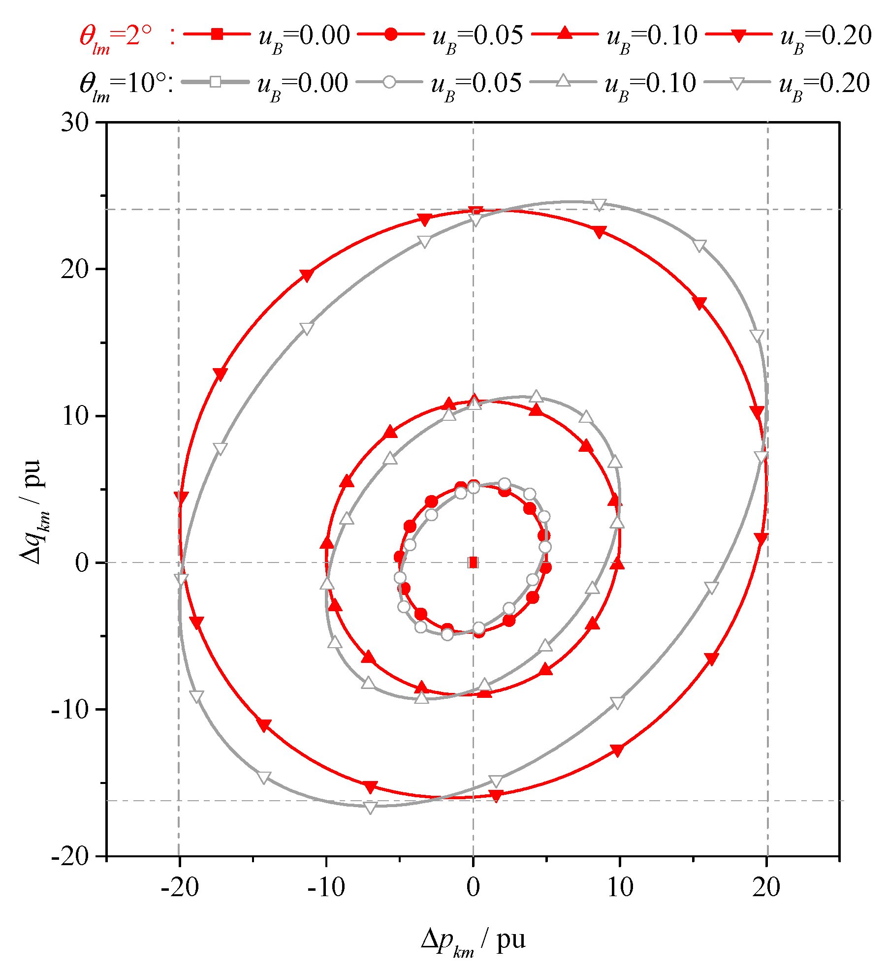
To show the UPFC regulation capability in different situations, the $\Delta p_{km}$-$\Delta q_{km}$ curves under different u_B and ${\theta }_{lm}$ are calculated using Equation (5), and presented in Figure 2. In the calculation, x_lm is 0.01 p.u., u_l and u_m are both 1 p.u. u_B in Figure 2 is in p.u.

It is demonstrated that the $\Delta p_{km}$-$\Delta q_{km}$ curves are ellipses. Besides, as shown in Figure 2, the area of the ellipse (that is, the regulation region of the power flows) will increase greatly with the increase of u_B. Under different ${\theta }_{lm}$, the maximum and minimum values of $\Delta p_{km}$ remain unchanged, and are always opposite to each other; but the maximum and minimum values of $\Delta q_{km}$ change with ${\theta }_{lm}$, when ${\theta }_{lm}$ increases, the range of $\Delta q_{km}$ increases too. These results verify the conclusions of the previous analysis.

3. Key Factor Analysis

3.1. Interaction between the UPFC and the External System

In the analysis of the previous section, it is assumed that the voltage magnitudes and phase angle difference of the line terminals remain unchanged. However, in practical power grids, they change with the power flow regulation of the UPFC. To illustrate the impact of these changes, this section takes the system shown in Figure 3 as an example for analysis.

Assume that when the UPFC regulates the power flow of the transmission line, the active power delivered through the transmission cross-section, where the UPFC installation line is located, remains unchanged. Then, when the UPFC regulates the active power flow of the UPFC-embedded line, the active power flow of the other line in the transmission section will change, and thus the phase angle difference between bus l and bus m will change. According to (4), the change of ${\theta }_{lm}$ will change the initial active power flow of the UPFC-embedded line (i.e., p_km0). Specifically, when the UPFC increases p_km, the active power flow of the other line in the transmission section will decrease, resulting in a reduction of ${\theta }_{lm}$. The reduction of ${\theta }_{lm}$ in turn reduces the initial active power flow of the UPFC-embedded line, and thus hinders the UPFC from increasing p_km. Conversely, when the UPFC reduces p_km, the active power flow of the other line in the transmission section will increase, resulting in an increase of ${\theta }_{lm}$. Then, the increase of ${\theta }_{lm}$ in turn increases the initial active power flow of the UPFC-embedded line and hinders the UPFC from reducing p_km. It can be observed that the change of ${\theta }_{lm}$ will always hinder the UPFC from regulating the active power flow and thus reducing the active power flow regulation range of the UPFC-embedded line.

On the other hand, the shunt converter can provide reactive power support for bus l, so u_l can be maintained to a certain extent. However, for bus m, when the UPFC increases the reactive power flow of the UPFC-embedded line, the reactive power injected into bus m increases, which will cause u_m to increase. The increase of u_m will in turn hinder the increase of q_km. Conversely, when the UPFC reduces q_km, u_m will decrease, which will in turn hinder the decrease of q_km. According to Equation (4), the change of u_m leads to the change of the initial reactive power flow of the UPFC-embedded line (i.e., q_km0), and hinders the UPFC from regulating the reactive power flow, and thus reduces the reactive power flow regulation range.

According to the above analysis, after the changes in the voltage magnitude and phase angle difference of the line terminals are considered, the initial power flows of the UPFC-embedded line will change, and this moves the center of the p_km-q_km curve, resulting in the p_km-q_km curve no longer being a standard ellipse for the general cases. Besides, because the change in the center of the p_km-q_km curve always hinders the UPFC from regulating the power flow of the transmission line, the regulation range of the power flow is smaller than that of the ideal case.

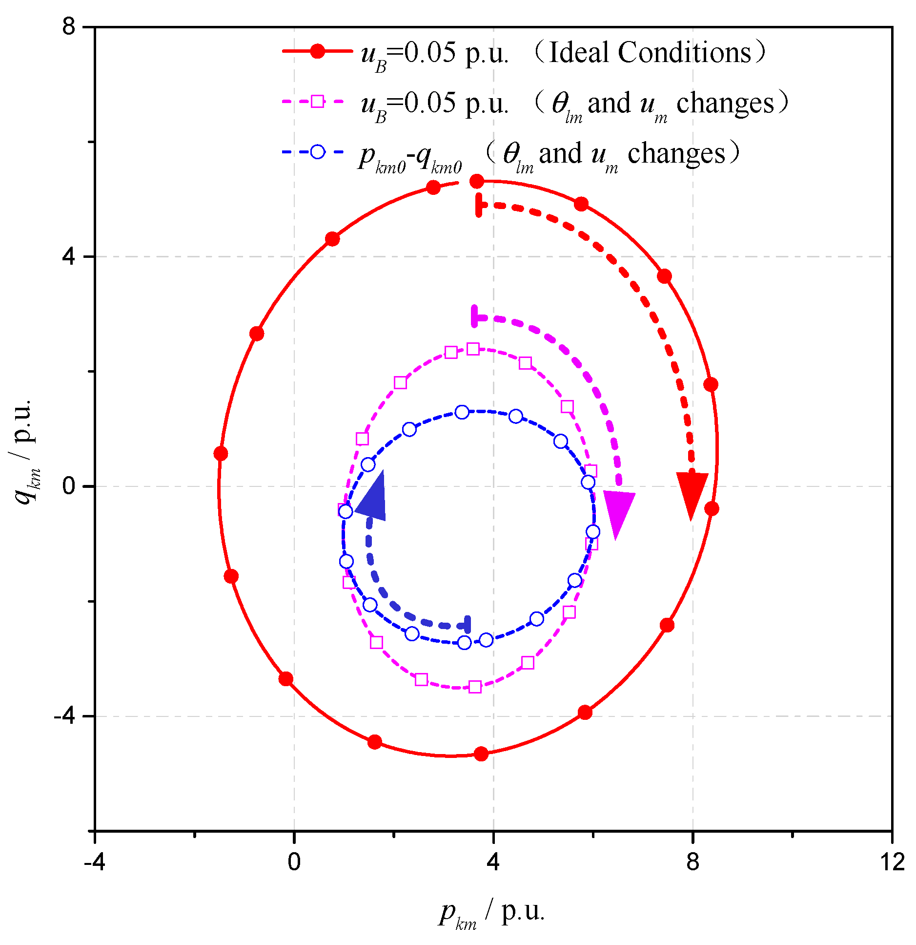
In order to verify the above conclusions, power flow calculations are conducted for the system shown in Figure 3. The parameters are set as follows: x_s = x_r = 0.02 p.u., x_lm = x_lm2 = 0.01 p.u., and p_s = p_r = 7 p.u. Under the above conditions, when u_B = 0, the initial active power flows of both transmission lines are 3.5 p.u., q_km0 is −0.71 p.u., and ${\theta }_{lm}$ is about 2°. When u_B = 0.05 p.u., the power flows of the UPFC-embedded line under different ${\theta }_{Bm}$ are calculated. 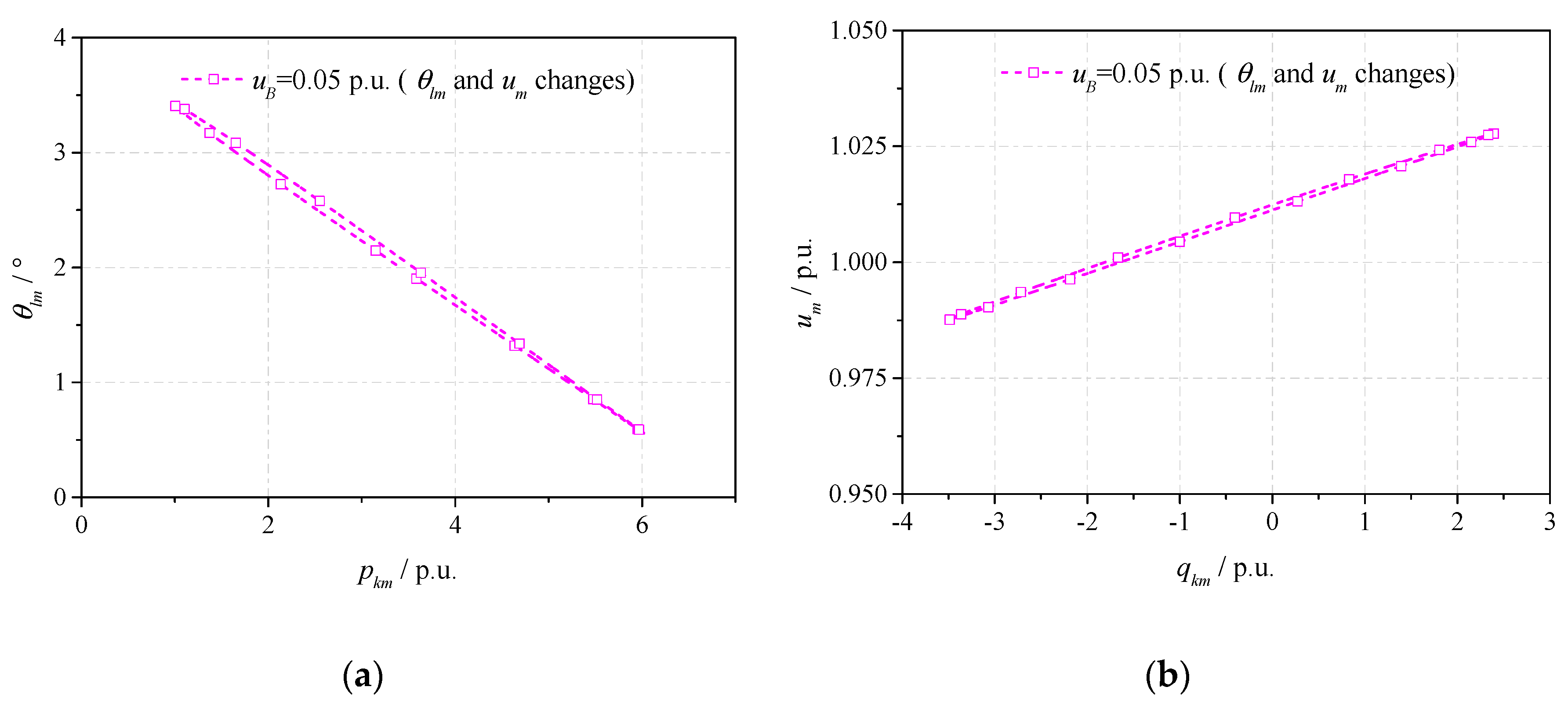The p_km-q_km curves and p_km0-q_km0 curves are shown in Figure 4. The p_km-θ_lm curve is shown in Figure 5a, and the q_km-u_m curve is shown in Figure 5b.

As shown in Figure 4, the change direction of the initial power flow curve (p_km0-q_km0) is about 180° different from that of the line power flow curve (p_km-q_km). This hinders the change of the line power flow and reduces the power flow regulation range significantly.

After the changes of θ_lm and u_m are considered, the range of p_km changes from −1.5 p.u. ~ 8.5 p.u. to 1.0 p.u. ~ 6.0 p.u. The range has been reduced by 5 p.u. At the same time, as shown in Figure 5a, when p_km increases, θ_lm decreases. The range of θ_lm is 0.56° ~ 3.43°. According to Equation (4), the change of the initial active power flow caused by the change of θ_lm is about 5 p.u., which is consistent with the change in the active power flow regulation range in Figure 4. This means the change of θ_lm is the main reason for reducing the regulation range of p_km.

As shown in Figure 4, after the changes of θ_lm and u_m are considered, the range of q_km changes from −4.7 p.u. ~ 5.3 p.u. to −3.5 p.u. ~ 2.4 p.u. The range has been reduced by about 4 p.u. At the same time, as shown in Figure 5b, when q_km increases, u_m increases. The range of u_m is 0.988 p.u. ~ 1.022 p.u. According to Equation (4), the change of the initial reactive power flow caused by the change of u_m is about 4 p.u., which is consistent with the change in the reactive power flow regulation range in Figure 4. This means the change of u_m is the main reason for reducing the regulation range of q_km.

According to the above analysis, the changes in the voltage magnitude and phase angle difference of the line terminals will reduce the regulation range of the power flow, so if we use the ideal conditions to analyze the power flow regulation capability of the UPFC in actual power grids, there will be large errors in the results. As the changes of the voltage magnitude and phase angle difference are related to the network structure and line parameters, the influence of these factors on the UPFC power flow regulation capability should be considered. Besides, as shown in Figure 5a, the p_km-θ_lm curve is approximately a straight line. Using this feature, the active power regulation range of the UPFC can be further analyzed. The specific content will be given in Section 4.

3.2. Impact of Constraints

In addition to the above factors, the UPFC power flow regulation capability in actual power grids is also restricted by many constraints, mainly including the rated current of the UPFC series converter, the line rated current, the constraint of the exchange power between the UPFC series converter and the shunt converter, the constraint of the shunt converter capacity. Due to these constraints, the allowable range of the line power flow may be further reduced.

Specifically, in order to ensure that the transmission capacity of the UPFC-embedded line will not be reduced, the rated current of the UPFC series converter is usually equal to the line rated current [14]. Therefore, these two current constraints can be considered together. Since the bus voltages in practical grids are around their rated values, the rated current constraint approximately corresponds to a circle in the PQ plane. The area within the circle is allowable for the UPFC.

When the output of the shunt converter reaches the rated capacity (S_sht), the shunt converter cannot continue to control the voltage magnitude of bus l. Similar to u_m, the change of u_l will also hinder the reactive power flow regulation of the UPFC, and reduces the reactive power flow regulation range.

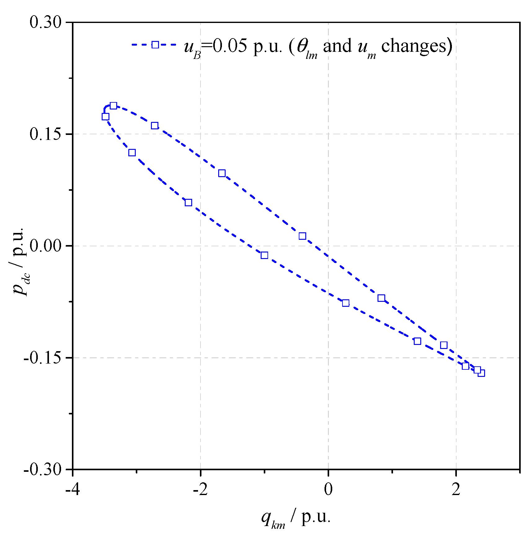
The exchange power between the UPFC series converter and the shunt converter may also limit the power flow regulation capability of the UPFC. According to Figure 1, the exchange power p_dc can be calculated as:

$$p_{dc}=p_{lm}-p_{km}=\mathrm{Re}\left[u_B\angle {\theta }_{Bm}{\left(\frac{u_k\angle {\theta }_{km}-u_m}{j{x}_{lm}}\right)}^{*}\right]$$

(14)

where Re denotes the real part of a complex number. Equation (14) can be simplified as:

$$p_{dc}=\frac{u_B}{x_{lm}}\left[u_l\sin \left({\theta }_{Bm}-{\theta }_{lm}\right)-u_m\sin \left({\theta }_{Bm}\right)\right]$$

(15)

Because u_l and u_m are approximately equal to 1 p.u., we have:

$$\begin{array}{ccc}{p}_{dc}& \approx & \frac{u_B}{x_{lm}}\left[\sin \left({\theta }_{Bm}-{\theta }_{lm}\right)-\sin \left({\theta }_{Bm}\right)\right]\\ & =& -\frac{2u_B}{x_{lm}}\cos \left({\theta }_{Bm}-{\theta }_{lm}/2\right)\sin \left({\theta }_{lm}/2\right)\end{array}$$

(16)

According to Equation (16), when ${\theta }_{Bm}$ is close to ${\theta }_{lm}/2$ (or ${\theta }_{lm}/2-180°$), the absolute value of p_dc (i.e., |p_dc|) reaches the maximum. At the same time, when ${\theta }_{Bm}$ is close to ${\theta }_{lm}/2$ (or ${\theta }_{lm}/2-180°$), the phase angle of u_B is between those of u_l and u_m (or −u_l and −u_m). If ${\theta }_{lm}$ is small, the absolute value of the d-axis component of u_B is much larger than the absolute value of its q-axis component, under the dq decomposition with the voltage of bus l as the reference. The d-axis component of u_B mainly affects the reactive power flow of the line [11]. When the absolute value of the d-axis component of u_B is large, |∆q_km| is also large. Therefore, when |p_dc| is relatively large, |∆q_km| is also relatively large. This means that the exchange power constraint may reduce the range of the line reactive power flow at this time.

For the system shown in Figure 3, the q_km-p_dc curve is shown in Figure 6.

As shown in Figure 6, when |∆q_km| increases, |p_dc| increases, but because a small u_B can make line power flow change in a wide range, the maximum of |p_dc| is much smaller than the maximum of |∆q_km| or |∆p_km|.

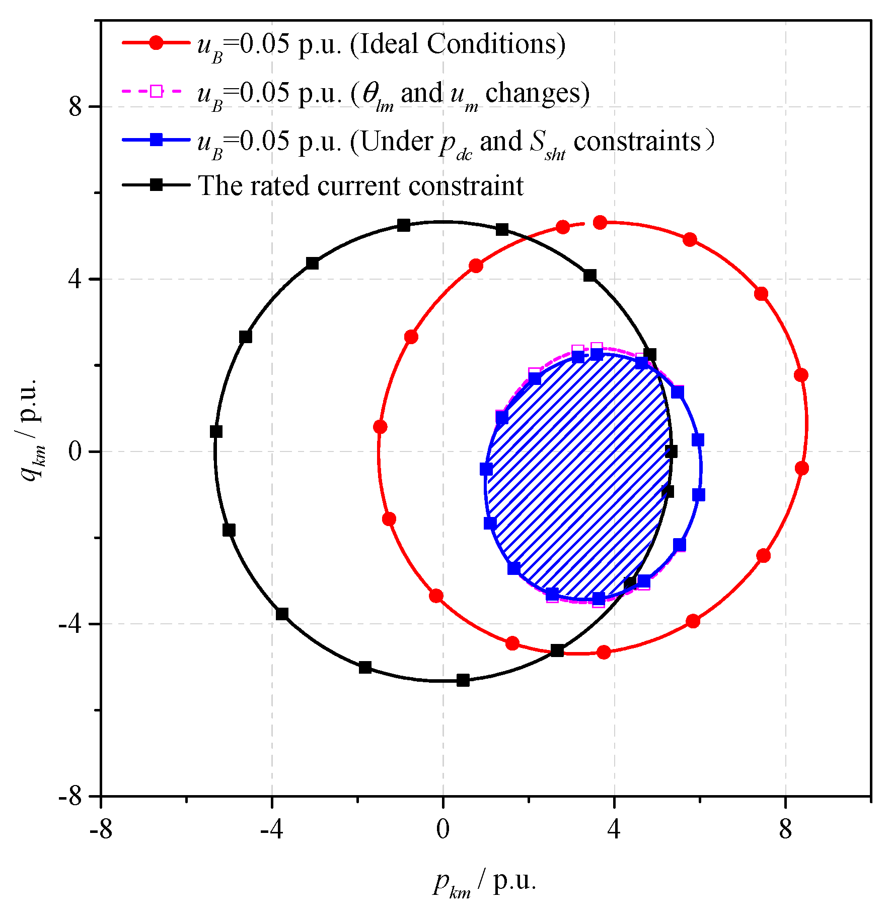
After considering all the above constraints, the feasible p_km-q_km region of the system in Figure 3 is presented in Figure 7. In the calculation, the rated capacity of Line 1 is 5.33 p.u., the rated current of the UPFC series converter is equal to that of the transmission line, the maximum exchange power between the series converter and the shunt converter is 0.2 p.u., S_sht is 0.5 p.u., and the maximum value of u_B is 0.05 p.u.

As shown in Figure 7, under the ideal conditions, the UPFC has the largest power flow regulation region. After considering the changes of ${\theta }_{lm}$ and u_m, both the active power flow range and the reactive power flow range are reduced. After considering the constraints of p_dc and S_sht, the reactive power flow range is further reduced. After considering the rated current constraint of the series converter, the power flow regulation region is limited by the solid black line. Finally, the feasible p_km-q_km region is the blue shaded area in the figure.

4. Active Power Flow Regulation Capability in Complex Power Grids

4.1. Relationship between UPFC Active Power Flow Regulation Capability and Grid Parameters

According to the analysis in the previous section, the active power flow regulation capability of the UPFC is mainly affected by the change in the phase angle difference of the line terminals. The relationship between the bus voltage phase angles and the power injections of the UPFC can be given by the DC power flow model [17]. For the UPFC embedded in line l-m (as shown in Figure 1), the power injection model of the UPFC is shown in Figure 8 [26].

When the losses of the UPFC and the transmission line are ignored, we have:

$$P_l=-P_m=-p_{km}$$

(17)

In DC power flow calculations, the phase angles of bus voltages can be calculated by [17]:

$$\mathit{\theta }={\mathit{B}}^{-1}\mathit{P}=\mathit{X}\mathit{P}$$

(18)

where θ is the vector of phase angles. B indicates the admittance matrix, and X is the inverse of B. P indicates net power injections.

According to Equation (18), there is a linear relationship between the voltage phase angles and the power injections of the UPFC, and the voltage phase angles of bus l and bus m can be represented by:

$$\{\begin{array}{l}{\theta }_l=a_l-b_l{P}_m\\ {\theta }_m=a_m-b_m{P}_m\\ {\theta }_{lm}=\left(a_l-a_m\right)-\left(b_l-b_m\right)P_m\end{array}$$

(19)

where a_l, b_l, a_m, and b_m are parameters related to the network structure and line impedances. b_l and b_m can be calculated by:

$$\{\begin{array}{l}{b}_l=X_{ll}-X_{lm}\\ b_m=X_{ml}-X_{mm}\end{array}$$

(20)

where X_ij is the element in the ith row and the jth column of X.

According to Equations (19) and (3), the relationship between P_m and ${\theta }_B$ is:

$$P_m=p_{km}=\frac{u_m{u}_l}{x_{lm}}\sin \left[\left(a_l-a_m\right)-\left(b_l-b_m\right)P_m\right]+\frac{u_m{u}_B}{x_{lm}}\sin \left[{\theta }_B-\left(a_m-b_m{P}_m\right)\right]$$

(21)

According to the derivative of Equation (21), we know that when $\cos \left[{\theta }_B-\left(a_m-b_m{P}_m\right)\right]=0$, P_m gets its maximum and minimum values. According to the extremum condition, if we treat ${\theta }_{Bm}$, which is equal to ${\theta }_B-\left(a_m-b_m{P}_m\right)$, as an independent variable, the extreme values of P_m will not be changed. At this time, Equation (21) becomes:

$$P_m=\frac{u_m{u}_l}{x_{lm}}\sin \left[\left(a_l-a_m\right)-\left(b_l-b_m\right)P_m\right]+\frac{u_m{u}_B}{x_{lm}}\sin {\theta }_{Bm}$$

(22)

According to Equation (22), we can easily obtain the extreme values of P_m by using software such as Wolfram Mathmetica. Besides, we can analyze the characteristics of the UPFC regulation capability under different a_l-a_m and b_l-b_m.

4.2. Estimation Method of the Active Power Flow Regulation Range

If the system structure and line parameters do not change, a_l-a_m and b_l-b_m are both constant. At this time, the extreme values of P_m can be estimated using the following method:

Step 1:

Input the system data before installing the UPFC. Calculate the admittance matrix (B) and its inverse matrix (X). Calculate the initial power flow without the UPFC, and obtain a set of θ_lm and P_m, denoted by θ_lm0 and P_m0.

Step 2:

Calculate b_l and b_m by Equation (20) using X obtained in Step 1.

Step 3:

Calculate a_l-a_m by Equation (19) using b_l-b_m obtained in Step 2 and θ_lm0 and P_m0 obtained in Step 1.

Step 4:

Calculate u_B according to the capacity of the UPFC series converter.

Step 5:

Set u_l and u_m to 1 p.u., calculate the extreme values of P_m by Equation (22).

Using the above method, we can easily estimate the active power regulation range of the UPFC, without conducting any power flow calculation for the power system with the UPFC.

4.3. UPFC Regulation Capability under Different Grid Parameters

The characteristics of the UPFC regulation capability under different grid parameters can be analyzed according to Equation (22). Specially, if we keep a_l-a_m = 0.1 (about 5.7°), x_lm = 0.01 p.u., and u_B = 0.1 p.u., then when b_l-b_m changes from 0.00 to 0.05, P_m under different ${\theta }_{Bm}$ can be calculated according to Equation (22). The results are shown in Figure 9.

As shown in Figure 9, the change of b_l-b_m will affect the range of P_m (that is, the difference between the maximum and the minimum of P_m). The larger b_l-b_m means the greater the change of θ_lm with the UPFC active power flow regulation. As a result, the range of P_m decreases with the increase of b_l-b_m. When b_l-b_m is zero, the range of P_m is the largest.

On the other hand, if we keep b_l-b_m = 0.01, x_lm = 0.01 p.u., and u_B = 0.1 p.u., then when a_l-a_m changes from 0.0 to 0.5, P_m under different ${\theta }_{Bm}$ can be calculated according to Equation (22). The results are shown in Figure 10.

As shown in Figure 10, the ranges of P_m are almost the same under different a_l-a_m. When other conditions keep unchanged, the change of a_l-a_m has little effect on the range of P_m, but it will change the maximum and the minimum of P_m. When other conditions keep unchanged, the maximum and the minimum of P_m will increase with the increase of a_l-a_m (when (a_l-a_m) < π/2).

5. Case Study

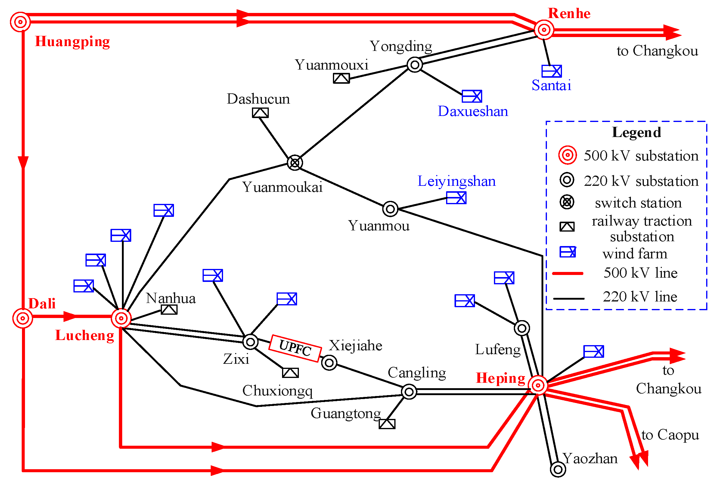
In other to verify the effectiveness of the estimation method and the correctness of the analysis results, the Chuxiong Power Grid, which is a practical power grid in China [26], is analyzed in this section. The schematic diagram of the Chuxiong Power Grid is shown in Figure 11. The base capacity of the system is 100 MVA. All per unit values given in this section are based on the system base capacity.

As shown in Figure 11, a UPFC is installed in the Zixi-Xiejiahe line. The capacities of the shunt converter and the series converter are both 40 MVA. The maximum output voltage of the series converter is about 0.125 p.u. The reactance of the Zixi-Xiejiahe line is 0.01197 p.u.

5.1. Calculation Process of the Estimation Method

In order to illustrate the calculation process of the estimation method, the UPFC regulation capability is analyzed under the typical operating condition (base case 1). Under this condition, the network structure is shown in Figure 11, and all line impedances are given, so the admittance matrix (B) of the system can be established, and its inverse matrix (X) can be calculated. Then, we have: X_ll = 0.01873, X_lm = X_ml = 0.006539, and X_mm = 0.03489. According to Equation (20), we have:

$$b_l=0.01219,b_m=-0.02835,b_l-b_m=0.04054$$

(23)

Before the UPFC is installed, the initial states of the system are: P_m0 = 2.6498 p.u., ${\theta }_{l0}$ = 14.3527° (0.2505 rad), and ${\theta }_{m0}$ = 12.5187° (0.2185 rad). Then, according to Equations (19) and (23), we have:

$$a_l=0.2828,a_m=0.1434,a_l-a_m=0.1394$$

(24)

If we set u_l = u_m = 1.0 p.u., u_B = 0.125 p.u., and x_lm = 0.01197 p.u., then according to Equation (22), the active power flow regulation range of the UPFC can be calculated, and the maximum and minimum values of the line active power flow are obtained, which are 5.036 p.u. and 0.267 p.u. respectively.

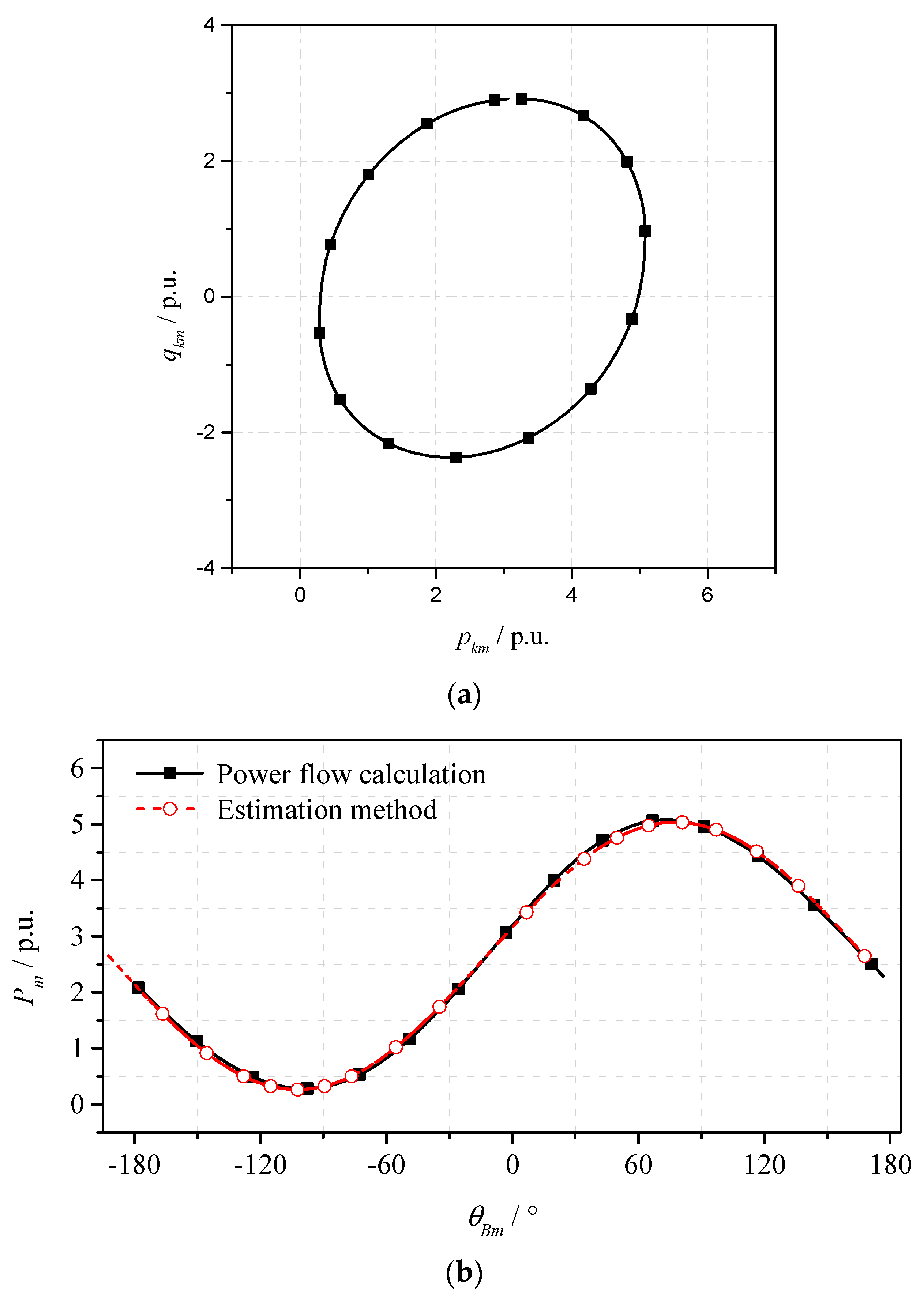
To verify the above results, power flow calculations are conducted using the fully coupled Newton-Raphson iterative algorithm in PSS/E. The voltage magnitude of the UPFC series converter is controlled to 0.125 p.u., and the voltage phase angle changes from −180° to 180°. The p_km-q_km curve obtained by power flow calculations is shown in Figure 12a. The active power flow under different ${\theta }_{Bm}$ is compared with the results obtained by the estimation method, as shown in Figure 12b. (For the convenience of the active power flow comparison, the curve of the estimation method is shifted to the left by 12.5°)

As shown in Figure 12a, the p_km-q_km curve approximates to an ellipse, which is similar to the result in Section 3. As shown in Figure 12b, the range of the active power flow obtained by the estimation method is nearly consistent with the result of the power flow calculations. The maximum and minimum values of the active power flow obtained by the power flow calculations are 5.081 p.u. and 0.285 p.u. respectively. The errors of the estimation method are 0.045 p.u. (4.5 MW) for the maximum value and 0.018 p.u. (1.8 MW) for the minimum value. The errors are small. The effectiveness of the estimation method is verified. Besides, according to Equation (13), the active power flow regulation range under ideal conditions is −7.793 p.u. ~ 13.093 p.u., which is much larger than the range obtained by the power flow calculations. This result confirms that it is necessary to consider the influence of the external system on the UPFC power flow regulation. Furthermore, as the errors of the estimation method are small, it is verified that the change in the phase angle difference of the line terminals is the main factor affecting the UPFC active power flow regulation capability.

The above results show that we only need to know the admittance matrix of the system and the power flow before installing the UPFC, and then we can quickly estimate the active power flow regulation range of the UPFC-embedded line after installing the UPFC according to Equation (22). There is no need to conduct any power flow calculation for the power system with the UPFC, which greatly reduces the requirements for the power flow calculation program.

In addition, if we calculate the regulation range by power flow calculations, the process of modifying the output voltage of the UPFC usually needs to be done manually. In order to obtain accurate results, the step of each adjustment of the phase angle could not be too large. For example, if we change the phase angle by 5 degrees at a time, we need to do a total of 72 power flow calculations. This makes the whole process cumbersome and time-consuming. If we adopt the estimation method, all these power flow calculations are avoided, thus the calculation process is greatly simplified.

5.2. UPFC Regulation Capability under Different Conditions

To analyze the characteristics of the UPFC and verify the estimation method under different grid parameters, the UPFC active power flow regulation range is calculated under different conditions.

5.2.1. Operating Condition 1

The active power flow of the Zixi-Xiejiahe line is required to be no larger than 280 MW, which is 2.80 p.u. on the system base capacity. Under the typical operating condition (base case 1), for all the single line outages that will overload the Zixi-Xiejiahe line, the UPFC active power flow regulation range is calculated. The estimation method results for all these contingencies are shown in

Table 1. Estimation method results under different contingencies.

No.	Contingency	al-am	bl-bm	Pmax	Pmin	∆Pmax	∆Pmin
0	Base case 1 (no outages)	0.1394	0.04054	5.036	0.267	−0.045	−0.018
1	Trip Lucheng-Heping	0.2055	0.04213	6.110	1.479	−0.062	0.008
2	Trip Lucheng-Cangling	0.2773	0.06256	5.398	2.036	−0.067	0.046
3	Trip Lucheng transformer	0.2153	0.04716	5.755	1.518	−0.026	−0.005
4	Trip Lucheng-Zixi #1 (or #2)	0.1693	0.04627	5.054	0.754	−0.040	0.004
5	Trip Lucheng-Yuanmoukai	0.1510	0.04158	5.155	0.478	−0.042	−0.012

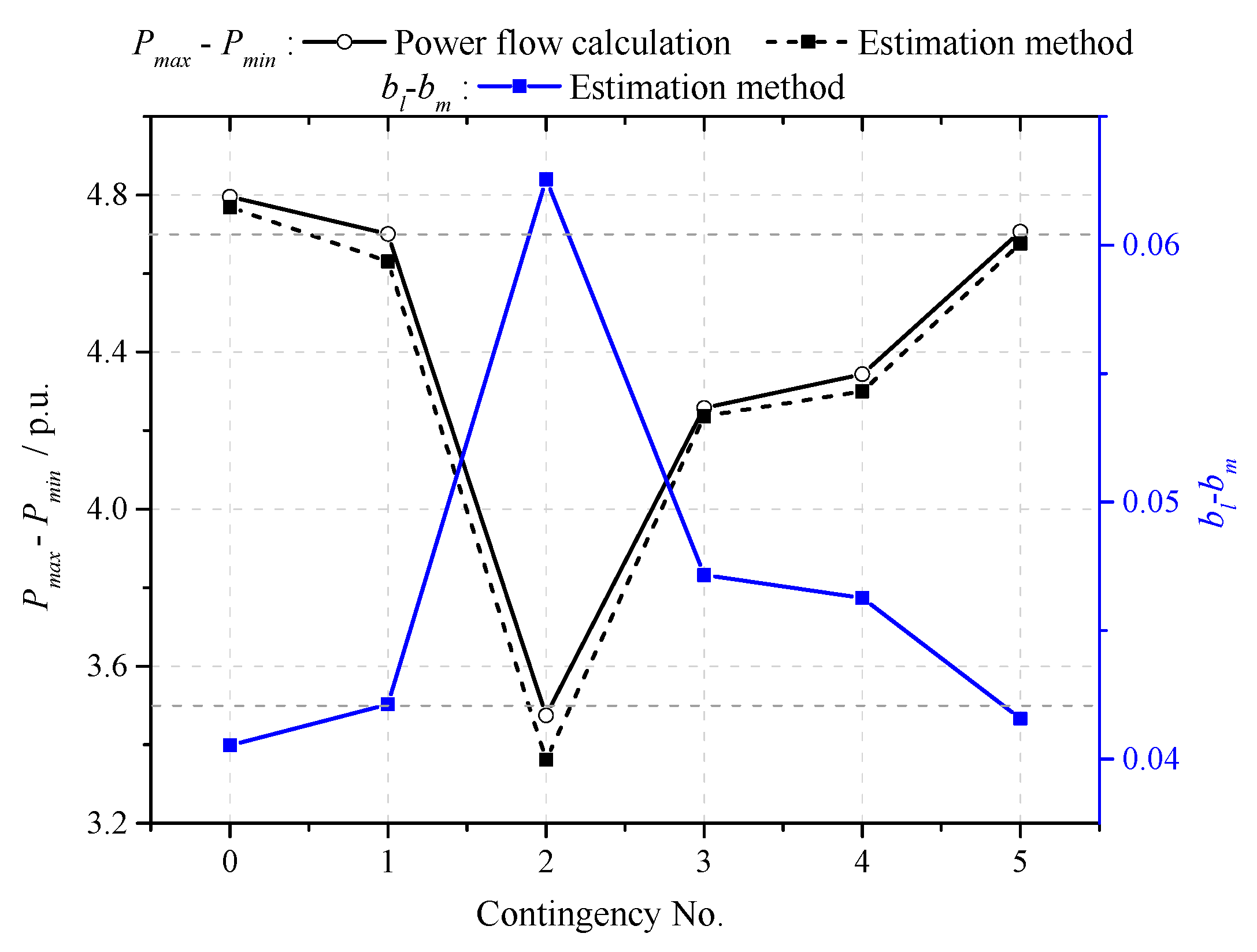
. The maximum and minimum values of the line active power flow are given in the columns of P_max and P_min respectively, and the errors of P_max and P_min between estimation method results and power flow calculation results are presented in the columns of ∆P_max and ∆P_min respectively. All data in the table are per unit values on the system base capacity. Besides, the curves of b_l-b_m and the range of P_m under different contingencies are shown in Figure 13.

As shown in Table 1, the maximum and minimum values of the line active power flow obtained by the estimation method are very close to the power flow calculation results. The maximum error of P_max and P_min is less than 0.07 p.u. (7 MW). This result further validates the effectiveness of the estimation method. Besides, it is shown that the UPFC has the ability to keep the line from being overloaded under all these contingencies, as P_min is always less than 2.80 p.u. (280 MW).

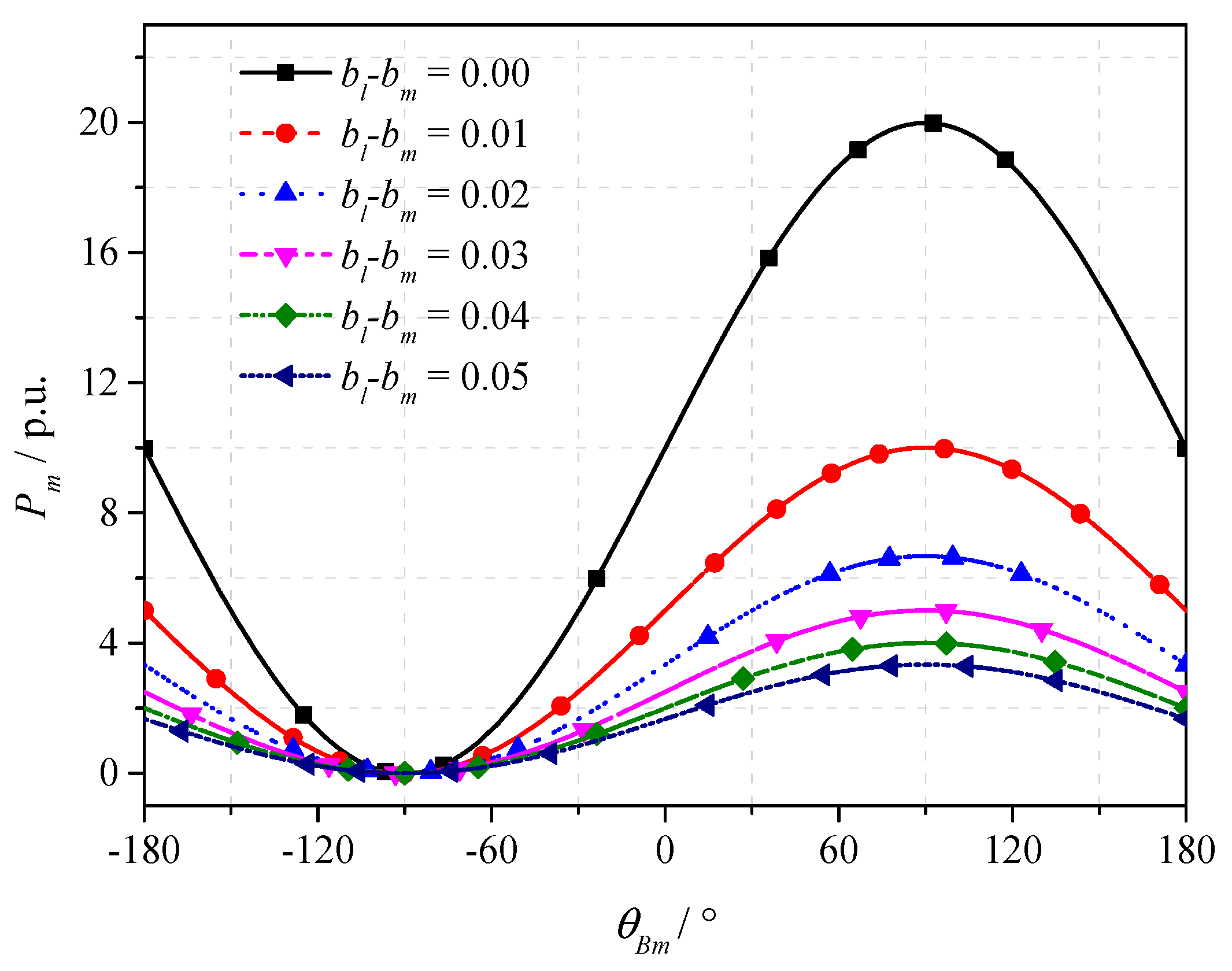
As shown in Figure 13, all the contingencies given in Table 1 will lead to the increase of b_l-b_m, and regardless of whether the power flow calculation method or the estimation method is adopted, P_max-P_min will always decrease with the increase of b_l-b_m. Besides, as shown in Table 1, by comparing the results under contingency 1 (trip Lucheng-Heping) and contingency 5 (trip Lucheng-Yuanmoukai), it can be seen that when the change of b_l-b_m is small, P_max and P_min increase with the increase of a_l-a_m. These results are consistent with the conclusions given in Section 4.3.

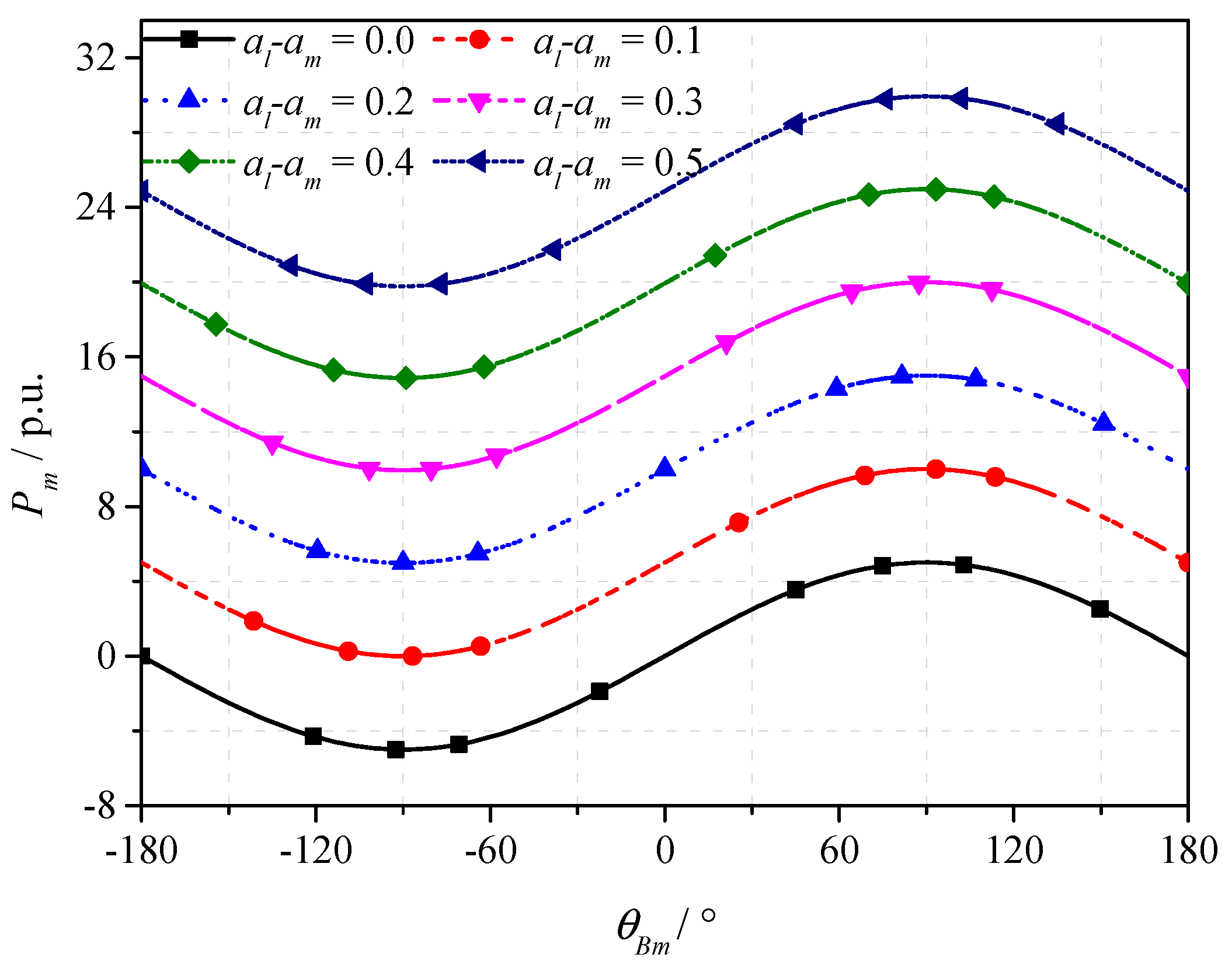
5.2.2. Operating Condition 2

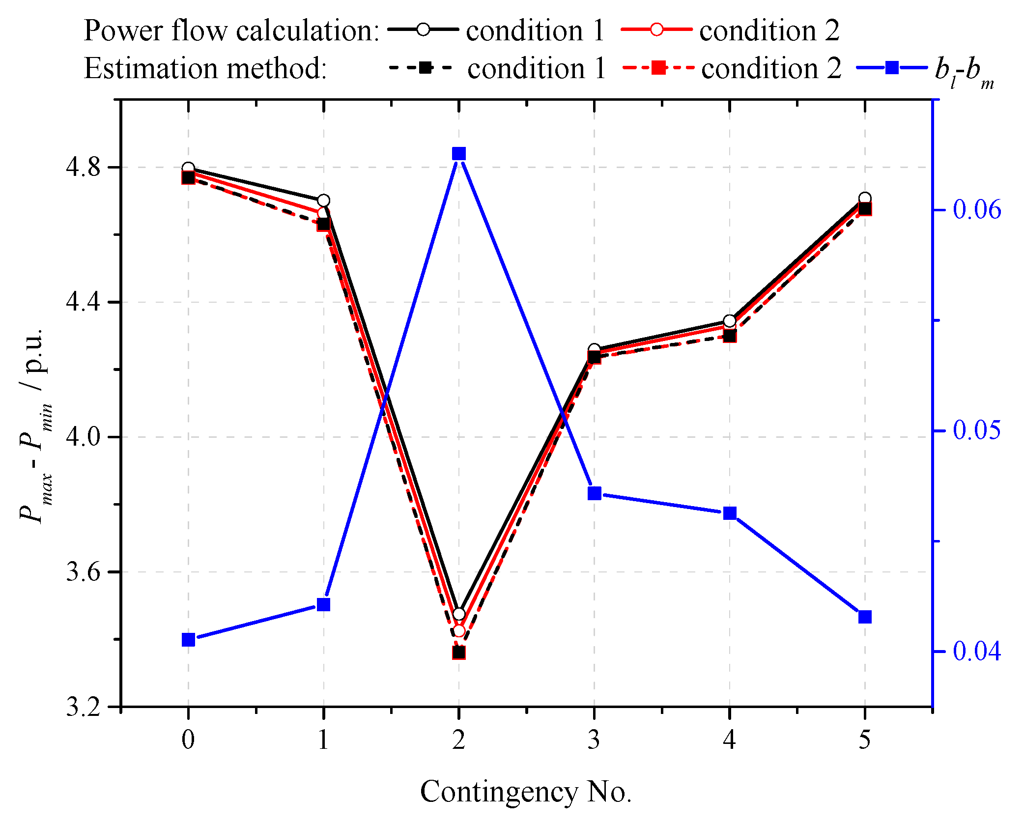
Under operating condition 2 (base case 2), the network structure is the same as that in operating condition 1, but the load of the system is reduced, and P_m0 = 1.7900 p.u. in the initial state. Similar to operating condition 1, the UPFC active power flow regulation range is calculated under different contingencies. The results of the estimation method are given in

Table 2. Estimation method results under operating condition 2.

No.	Contingency	al-am	Pmax	Pmin	∆Pmax	∆Pmin
0	Base case 2 (no outages)	0.0930	4.153	−0.615	−0.060	−0.043
1	Trip Lucheng-Heping	0.1552	5.180	0.551	−0.059	−0.025
2	Trip Lucheng-Cangling	0.1920	4.255	0.894	−0.066	−0.002
3	Trip Lucheng transformer	0.1193	4.133	−0.102	−0.044	−0.031
4	Trip Lucheng-Zixi #1 (or #2)	0.1067	3.981	−0.319	−0.055	−0.026
5	Trip Lucheng-Yuanmoukai	0.0985	4.175	−0.500	−0.059	−0.038

. The curves of b_l-b_m and the range of P_m are shown in Figure 14. It should be noted that because the network structure and line parameters are unchanged, for the same contingency, b_l-b_m under operating condition 2 is the same as that under operating condition 1, so the column of b_l-b_m is not presented in Table 2.

As shown in Table 2 and Figure 14, the following conclusions are verified: (1) the estimation method is effective under operating condition 2, as the errors of P_max and P_min are small (less than 0.07 p.u.); (2) all the contingencies given in Table 2 will increase b_l-b_m, and with the increase of b_l-b_m, P_max-P_min decreases; (3) for the same contingency, P_max-P_min in operating condition 2 is almost the same as that in operating condition 1, as b_l-b_m is unchanged; (4) by comparing the results under contingency 1 and contingency 5, it is shown that when the change of b_l-b_m is small, P_max and P_min increase with the increase of a_l-a_m.

The above results further validate the theoretical analysis and the estimation method. Besides, it is shown that if the network structure and line parameters are unchanged, it is very convenient to use the estimation method to analyze the UPFC regulation capability under different operating conditions, because there is no need to recalculate b_l-b_m, and we only need to know the initial states before the UPFC is installed.

6. Conclusions

The research on UPFC power flow regulation capability is of great significance for the design and operation of UPFC projects. This paper studies the UPFC regulation capability under different system conditions, and analyzes the influence of different factors on the UPFC regulation capability. Besides, an estimation method for the UPFC active power flow regulation range is proposed and verified. The following conclusions are drawn:

(1)

Under the ideal conditions, the dispatch trace of the UPFC at a constant injected voltage magnitude is usually an ellipse in the PQ plane. The regulation range of the line active power flow is independent of the sending-end bus voltage and the phase angle difference between the line terminals, but it is proportional to the magnitude of the UPFC injected voltage, and is inversely proportional to the line impedance. The regulation range of the line reactive power flow is related to the sending-end bus voltage and the phase angle difference between line terminals, and is also inversely proportional to the line impedance.

(2)

After the changes in the voltage magnitude and phase angle difference of the line terminals are considered, the regulation range of the UPFC will be reduced. The decrease of the active power regulation range is mainly affected by the change in the phase angle difference, while the decrease of the reactive power regulation range is mainly affected by the change in the voltage magnitude.

(3)

The UPFC power flow regulation capability in actual power grids is restricted by many constraints. The constraints of the shunt converter capacity and the exchanged power between the converters may reduce the reactive power regulation range, while the rated current of the UPFC series converter may reduce both the active and reactive power regulation range.

(4)

The active power flow regulation capability of the UPFC in practical power grids is not only related to the parameters of the UPFC and its installation line, but also related to the system structure and the parameters of other lines.

(5)

The active power flow regulation capability of the UPFC can be estimated by the method proposed in this paper. This method can lower the requirements for the power flow calculation program, and reduce computation load.

(6)

Line outages may increase b_l-b_m, and thus reduce the active power flow regulation capability of the UPFC.