Oil as Hedge, Safe-Haven, and Diversifier for Conventional Currencies

Abstract

The research investigates the safe-haven, hedging, and diversification function of crude oil for conventional currencies, among which five are major oil exporters, and six are major oil importers. In order to model time-varying dynamic correlations between crude oil and currencies, the study uses the Asymmetric-DCC model. The findings highlight low or negative correlations, especially during the crisis period. Next, we employ a quantile based regression framework and conclude distinct safe-haven and hedge functions of oil for major currencies. We provide additional evidence on the safe-haven, hedging, and diversification function of crude oil using the cross-quantilogram framework. The findings of out of sample analysis illustrate that the hedging effectiveness of oil is greater for oil-exporting countries. In addition, the conditional diversification benefit of oil is higher in the lower quantiles, i.e., when both foreign exchange and oil markets are in a bearish state. Finally, implications for investors, portfolio managers, and policymakers are further discussed.

1. Introduction

In recent times, the foreign-exchange (FX) market has witnessed severe turmoil with dramatic movements noted in major currencies like the US Dollar, Swiss Franc, Canadian Dollar, and Russian Ruble. More importantly, the ever-increasing volatility in the FX market holds alarming repercussions for market participants. Since the dramatic variations in exchange rates significantly influence the dollar value of the company’s balance sheet items denominated in foreign currencies, central banks across countries have introduced policy measures to stabilize the macroeconomic environment to shield against risks arising from the exchange rate volatility. Still, many assert that such interventions weaken the notion of free flow of goods and services across-borders, and rather more attention needs to be devoted to understanding the drivers of FX market volatility. In this view, fluctuations in commodity prices are cited among major drivers of the volatility in the FX market. Without doubt, the most prominent commodity affecting the dynamics of the economy and trade is crude oil. It is well recognized that in both oil-importing and exporting countries macroeconomic variables like GDP, inflation, stock prices, trade imbalances, and exchange rates are enormously influenced by crude oil price dynamics [1]. Additionally, since the US dollar is predominantly used as invoicing and settlement currency for crude oil trade, the changes in the exchange rate of the local currency against the US dollar implies that forex capital is transferred between two economies based on the crude oil trade.

Theoretically, the currency–oil nexus is well established. Numerous studies have documented the currency–oil nexus dynamics using a variety of methods and data sets [2,3,4,5,6].

Earlier studies identify three channels with which crude oil prices affect the currency dynamics. The known channels include terms of trade introduced by [7], portfolio reallocation, and wealth effects described by [8,9,10]. First, the trade term concept explains the currency–oil link by terming crude oil as a key driver of trade. In countries with significant oil dependence, when oil prices increase, the tradable sectors are largely affected. Consequently, currency and nominal exchange rate depreciate due to high inflation. However, in case of oil-exporting countries, the underlying phenomena generates improvement in trade balance and strengthening of the local currency. Still, this appreciation of currency adversely impacts non-oil sectors by reducing the level of exports in the long-run. This is known as the Dutch disease phenomenon. The remaining two channels also highlight the influence of oil prices variations on conventional currencies. Wealth effects explain the short term impact and portfolio reallocation channel covers medium and long-term effects of oil prices on currency dynamics. Accordingly, higher oil prices are believed to create wealth transfer from oil-importing economies to oil-exporting economies. Hence, increase in crude oil prices implies appreciation of exchange rates for oil-exporting economies and vice versa for oil-importing economies.

This is also well known that exchange rates can significantly influence crude oil prices through changes in demand and supply of crude oil linked to the role of USD. Considering the supply side, a decrease in USD value encourages oil-exporting economies to reduce the oil supply and increase oil prices to maintain the purchasing power value of their exports in USD terms. In the same way from a demand-side view depreciation in USD implies less expensive oil imports in terms of the local currency which increases the oil demand outside the US and stimulates subsequent rise in oil prices. Similarly, for many years, academics and market practitioners have also corroborated the idea that appreciation in USD causes lower oil prices [11]. Additionally, a vast literature has comprehensively highlighted the common factors driving exchange rates and oil prices, which include GDP, interest rates, inflation stock price volatility, policy uncertainty, and geopolitical risks [12,13,14].

While researchers have extensively studied the dynamic links between oil prices and currencies, nevertheless, due to several factors including profound volatility in FX and crude oil market, financialization of the oil market after the mid-2000s and unprecedented increase in the level of risk and uncertainty post-Global Financial Crisis (GFC) has renewed interest in understanding the oil–currency nexus. Although their own set of systematic risks influence currencies and oil prices, still, the underlying factors that drive the market risk in one market also serve as a catalyst of risk in the other market. Moreover, the feedback mechanism between the underlying markets gives rise to strong currency–oil connectedness [15]. Given the strong theoretical link between the two markets based on earlier described transmission channels, it is worthwhile to imply that currency appreciations and depreciations have a significant impact on oil prices and vice versa. Further, the inverse relationship between oil and FX market also highlights the likelihood of using oil to hedge currency fluctuations or utilize as a safe-haven asset for extreme currency movements.

Customarily, commodities are acknowledged as effective hedgers against the downward moments in other asset classes, particularly gold and oil. The hedge and safe-haven function of gold and WTI crude oil for different financial assets is documented by numerous studies [16,17,18,19], among others. Particularly, in terms of gold and FX market dynamics, gold is considered disinflationary and serves as a safe-haven and hedge asset for currency devaluations [20,21]. Evidence also shows that gold-currency portfolios are useful for portfolio diversification and downside risk reduction [22]. However, there exists a scarce literature on the hedging and safe-haven function of WTI crude oil for conventional currencies. To the best of our knowledge, the earlier literature on currency–oil nexus has not addressed this question. Additionally, due to the recent rapid financialization of the crude oil market and strong informational dependencies between the two underlying markets, there is a likelihood that oil prices sufficiently serve as a risk-hedging tool for currency appreciations and depreciation. Moreover, crude oil financialization enables portfolio managers to utilize crude oil for currency portfolio risk management. In a nutshell, no earlier study asks the question whether crude oil prices constitute effective diversifier for the currencies risk.

Within the thematic focus of this growing body of literature, this study motivates to examine the diversification, safe-haven, and hedging potential of crude oil for major currencies, among which five are major oil exporters, and six are major oil importers. In a nutshell, we explore following research questions: (1) is the crude oil an effective diversifier for currency portfolios? (2) Is the crude oil a strong or weak hedge or safe-haven asset for currency fluctuations? The paper follows four steps to examine the effectiveness of crude oil for currency portfolio risk management. Firstly, we use the framework in [17] to investigate the potential safe-haven and hedging role of crude oil commodities for major currencies. Secondly, we model time-varying dynamic correlations between crude oil and major currencies using the ADCC-GARCH model. Additionally, we use rolling window analysis to formulate an out-of-sample forecast of optimal hedge ratios to examine the hedging effectiveness of crude oil. Thirdly, to assess conditional diversification benefits of oil together with major currencies, we utilize the test proposed by [23,24]. Moreover, portfolio analysis of this nature includes optimal weights, hedge ratios, and hedging effectiveness, which provide meaningful insights for currency risk management and portfolio diversification strategist. Finally, to trace the dependence structure between oil and the FX market across various quantiles, we also apply the cross-quantilogram approach proposed by [25]. Understandings of the informational interdependencies across both markets have significant cross-market implications for policymakers and market participants.

The empirical evidence exhibits strong safe-haven and hedge function of crude oil for the majority of the currencies and rejects the null hypothesis of a linear relationship with the conventional currencies over the sample period of the study. Further, the additional evidence obtained from the cross-quantilogram framework also corroborates the safe-haven and hedging function of crude oil for currency fluctuations. The out-of-sample hedging effectiveness of oil is higher for oil-exporting countries. Furthermore, the conditional diversification benefit of the oil is higher in the lower quantiles, i.e., when both currency and oil markets are in a bearish state. Overall, the findings show the risk management consequences of the link between crude oil and FX market and validate the use of crude oil for risk management of currency portfolios.

The rest of the paper is organized as follows: in Section 2, we briefly cover the literature on the topic, and Section 3 of the study discusses the methodologies. Section 4 illustrates the data and empirical findings of the study. The last section concludes the study with implications for investors and other market participants.

2. Literature Review

A large thread of theoretical and empirical research literature has covered the currency–oil nexus. The existing literature on the topic follows the conceptual association proposed by the early studies of [8,9,26], who reason that oil prices have an explanatory effect on exchange rates. Nevertheless, it is still important to understand that both crude oil and currencies are driven by several factors that are difficult to forecast. For instance, the exchange rate disconnect puzzle highlights the unstable association between exchange rates and macroeconomic fundamentals [27]. Similarly, the prediction of crude oil price fluctuation cycles is an onerous task due to demand and supply shocks. Further, since the American dollar serves as the settlement and billing currency in crude oil market, the major share of the earlier literature has mainly concentrated on the connection between crude oil and USD [28,29,30,31]. Hence, fluctuations in USD are taken as a crucial driver of crude oil prices. On the contrary, only a small fraction of research has explored the interconnection between oil and currencies in other countries.

Over the past two decades, currency–oil dynamics have been studied by many researchers using a variety of empirical methods. Still, the obtained evidence varies according to the sample, econometric method, and market. Most early studies on the topic use cointegration tests to validate the long-term association between the crude oil prices and exchange rates [32,33,34]. The results exhibit a significant long-term association between the two underlying variables, particularly for economies with significant oil dependence. Similarly, some studies model the causal links between crude oil prices and exchange rates using different modifications of Granger causality tests, but there is a lack of agreement about the direction and magnitude of the causal links. Firstly, in accordance with the wealth effect and terms of trade channel, the authors of [2,3] argue that crude oil prices significantly explain the changes in currencies for different countries. On the other side, others advocate that exchange rates cause crude oil prices, particularly the role of the American dollar as the billing and settlement currency is vital [35,36,37]. Whereas, a series of studies also document the bi-directional causal association between crude oil prices and currencies [38,39]. On the contrary, the authors of [40] find evidence of no causal connection between the two markets.

A long list of papers also examine the co-movements and dependence structure between oil prices and currencies by considering different econometric techniques. Overall, the findings obtained from different methodologies show negative correlations between oil prices and exchange rates [41,42,43]. Similarly, the nonlinearities of currency–oil nexus are also comprehensively addressed by studies using a variety of nonlinear frameworks. The authors of [44] find bi-directional causality between crude oil prices and exchange rates in China and India by employing nonlinear Granger causality tests. Few studies also use copula specifications to estimate the intensity of the nonlinear relationship and tail dependence between crude oil prices and currencies [45,46]. The results highlight the time-varying association between oil and conventional currencies. In particular, higher correlations are also observed during the Global Financial Crisis (GFC) period.

Further, studies of [5,47,48] document the volatility spillover transmission between the crude oil market and the FX market. The findings illustrate the volatility interaction between the underlying markets tends to be high during periods of economic downturn. Furthermore, some studies also validate the asymmetric linkages between crude oil prices and exchange rates using a variety of econometric methodologies [28,49].

Some recent studies employ wavelet methods to simultaneously model the association between oil and currencies in time and frequency domains. Using wavelet multi-resolution analysis, the authors of [6] find significant nonlinear association between Indian rupee and crude oil prices at lower frequencies. Further, in [50] the authors use a discrete wavelet transform approach and find higher contagion and negative interdependence between the crude oil and FX markets after GFC 2007–2008. Additionally, the authors of [51] use continuous wavelet analysis to explore the association between the oil and exchange rate in Japan. The findings indicate strong correlations between the two underlying variables in the sample period, but the magnitude of co-movement differs in different time horizons. Using the similar approach, in [52] the authors examine the co-movement between crude oil prices and exchange rates for leading oil-importing and exporting markets. The findings unveil strong correlations between currencies and oil prices for oil-exporting countries, and the linkages were even stronger during GFC. Additionally, the authors of [53] attempt to understand the dependence structure and systematic risk between crude oil prices and currencies of BRICS economies using quantile coherency methods. The findings confirm significant negative dependence in the long run between the crude oil and currencies of countries, namely India, South Africa, and Brazil. Finally, another strand of studies also examine the asymmetric spillovers and volatility connectedness between the FX market and crude oil market [5,48,54]. In addition, the authors of [15] also look at the directional and dynamic connectedness between crude oil prices and currencies of nine counties. The findings highlight that currency–oil pair connectedness is dominated by the oil market.

Interestingly, as it is evident from the literature despite enormous attention devoted to understanding the linkages between currency–oil nexus, none of the earlier studies have evaluated the possibility of taking different offsetting positions across both markets to create effective hedging and diversification opportunities for investors. Thus, the study takes a different perspective on the association between crude oil and currencies. This study contributes to the literature in two different ways. First, we test the potential hedging and safe-haven functions of crude oil for major currencies using different robust methods. Second, we also provide evidence on conditional diversification benefits of adding oil to currency portfolios.

3. Materials and Methods

Our study employs daily data of a wide range of FX future markets consisting of Canadian Dollar, Brazilian Real, Norwegian Krone, Mexican Peso, Russian Ruble, Euro, Japanese Yen, Swedish Krona, South African Rand, South Korean Won, Great Britain Pound, and the Indian Rupee. We sampled all these currencies with respect to the US Dollar. Data for the WTI oil prices and sampled FX market is based on the daily frequency and ranges from 3rd January 2000–30th August 2019. Data for both the series, i.e., WTI oil and FX market, was taken from Thomson Reuters DataStream. The descriptive statistics for WTI Crude oil and sample currencies is presented in

Table 1. Descriptive statistics for sample currencies and crude oil prices.

	Abbreviations	Mean (%)	Std. Dev. (%)	Skewness	Kurtosis	ADF
Canadian Dollar	CAN	−0.0017	0.5646	−0.0991	8.3189	−71.4893 ***
Japanese Yen	JPY	0.0007	0.6233	−0.2731	6.9980	−73.3252 ***
Indian Rupee	IND	0.0097	0.3772	0.2768	10.3234	−28.7705 ***
South African Rand	SAF	0.0176	1.0478	0.2793	7.9142	−69.6784 ***
Russian Ruble	RUS	0.0172	0.7637	0.2676	72.1643	−19.7453 ***
Euro	EUR	−0.0018	0.6008	−0.1382	5.7110	−70.9120 ***
Mexican Peso	MEX	0.0146	0.6729	0.7215	13.9545	−69.9721 ***
Brazilian Real	BRA	0.0163	0.9980	0.1168	14.4972	−54.2272 ***
Norwegian Krone	NOR	0.0024	0.7380	0.0009	7.4033	−71.5517 ***
South Korean Won	SKR	0.0013	0.6423	−0.6370	59.5435	−71.0671 ***
Swedish Krona	SWE	0.0027	0.7289	−0.1574	6.4526	−71.9072 ***
Great Britain Pound	GBP	0.0055	0.5865	0.5809	14.3042	−68.8710 ***
Crude Oil WTI	WTI	0.0149	2.3301	−0.1501	7.2822	−74.5314 ***

Note: ADF indicates the Augmented Dickey–Fuller test of stationarity. *** indicates significance at 1%.

. Among the FX market, South African Rand has a maximum daily return value of 0.0176%, whereas Euro exhibits a daily loss of 0.0018%. Variance in returns for all the currencies is quite high with South African Rand leading other currencies. South African Rand exhibits the highest variance of 1.0478%, whereas the Indian Rupee highlights the lowest variance of 0.3772. We see a mixed trend in the distribution of daily return values as Japanese Yen, South Korean Won, Canadian Dollar, and Euro exhibit negatively skewed behavior, whereas the rest of the currencies are positively skewed. The statistics for kurtosis are consistent for each currency, with each exhibiting leptokurtic distribution with fat tails.

Finally, unit root testing was executed using the ADF test and the stationarity assumption was rejected for daily return values of all the currencies. The average daily returns of WTI oil are 0.0149%, with a variance of 2.3301%. The WTI crude oil market exhibits negative skewness and leptokurtic distribution with fat tails and also possesses stationarity properties over the sampled period.

Our paper employs several estimation techniques pertinent to the objective of our study. We started our estimations by using the framework proposed earlier by [17] to investigate the safe-haven and hedging ability of oil commodities against the major currencies. This allowed us to model oil prices together with FX market assuming the presence of extreme market conditions. The model also provides for heteroscedasticity check to obtain consistent estimates. We proceeded by applying conditional diversification benefits of oil together with foreign currencies in a portfolio. This methodology allowed us to access diversification benefits of a portfolio comprising of oil and foreign currencies based on different varying proportions and under different levels of expected shortfall. Finally, we used cross-quantilogram based on the fact that the two markets (i.e., FX market and oil futures in our case) can simultaneously undergo different market conditions and therefore the underlying correlation exhibits a dynamic correlation pattern. The details and specification of each of the aforementioned methodologies are appended below.

3.1. Safe-Haven Testing

To explore the safe-haven functions of crude oil for major currencies, we apply the following principle regression functions as proposed by [17].

$$r_{Oil,t}=a+b_t{r}_{FX,t}+e_t$$

(1)

$$b_t=c_0+c_{1}D\left(r_{FX}{q}_{10}\right)+c_{2}D\left(r_{FX}{q}_5\right)+c_{3}D\left(r_{FX}{q}_1\right)+e_t$$

(2)

$$h_t=\pi +\alpha e_{t-1}^2+\beta h_{t-1}$$

(3)

Equation (1) presents principal regression function and is based on the assumption that oil prices are dependent on the changes in foreign exchange market. We also assume that the relationship between oil and the FX market is not constant and depends on extreme market conditions. In Equation (1), $a$ and $b$ represent coefficients which we need to estimate and $e_t$ denotes the error term. We estimate coefficient $b$ using the dynamic process given by Equation (2) however coefficients $c_0$, $c_1$, $c_2$, and $c_3$ are also required to be estimated. Equation (2) models $b_t$ as a dynamic process for capturing extreme market movements. The Expression $D(.)$ in Equation (2) represents dummy variables to capture movement in the FX market under different market conditions. If the returns in the FX market exceed the given threshold of 10%, 5%, or 1% of the quantile distribution, the dummy variables are given values of 1 and zero otherwise. However, if either of the dummy coefficients i.e., $c_0$, $c_1$, $c_2$, and $c_3$ are different from zero, this confirms nonlinear behavior of oil and the major currencies with each other. Furthermore, if all the estimated coefficients in Equation (2) turn out to be non-positive, then oil is considered to exhibit weak safe-haven properties for conventional currencies. In another case, if coefficients in Equation (2) have negative as well as different values than zero, oil exhibits strong safe-haven properties. Oil is also considered to exhibit safe-haven properties for the currencies if the coefficient $c_0$ is either negative or zero, however, the sum of coefficients from $c_1$ to $c_3$ should not have a positive value exceeding $c_0$. We apply GARCH (1,1) as specified in Equation (3) to check the presence of heteroscedasticity in our data series and follow the process of likelihood maximization for joint estimation.

3.2. Hedging Effectiveness

In order to check the hedging ability of crude oil for major currencies, we use hedging effectiveness measures. Moreover, the effectiveness of the hedged positions between oil and the FX market helps in investigating how much risk oil reduces in a combined portfolio. This process is quite effective and relevant as a measure of portfolio risk assessment (the process of hedging effectiveness is based on out of sample analysis.) Suppose $R_{H,t}$ represents returns on the hedged portfolio comprising of oil and FX futures.

$$R_{H,t}=R_{FX,t}-{\varnothing }_t{R}_{A,t}$$

(4)

where $R_{FX,t}$ denotes returns on the foreign exchange market, ${\varnothing }_t$ represents hedge ratio, and $R_{O,t}$ highlights returns on the oil market. The expression for hedged portfolio’s variance conditional on an informational set $I_{t-1}$ is presented as follows.

$$var\left(R_{H,t}{R}_{t-1}\right)=var\left(R_{FX,t}{I}_{t-1}\right)+{\varphi }_t^{2}var\left(R_{O,t}{I}_{t-1}\right)-2{\varphi }_{t}cov\left(R_{O,t},R_{FX,t}{I}_{t-1}\right)$$

(5)

We follow [55] in defining optimal coefficient by minimizing the conditional variance of the hedged portfolio as

$${\varphi }_t^{\ast }{I}_{t-1}=\frac{cov(R_{FX,t},R_{O,t}|I_{t-1})}{var(R_{O,t}|I_{t-1})}$$

(6)

We estimate hedge ratios using the extracted covariance and conditional volatility series using asymmetric generalized DCC-GARCH model by following the work of [56]. An expression for hedging a long position in FX futures by a short position in oil is appended below.

$${\varphi }_t^{\ast }{I}_{t-1}=\raisebox{1ex}{$h_{FXO,t}$}\!\left/ \!\raisebox{-1ex}{$h_{O,t}$}\right.$$

(7)

Equation (7) consists of $h_{FXO,t}$ which represents conditional covariance between oil and the FX future returns whereas $h_{O,t}$ denotes conditional covariance of oil returns. In order to estimate the optimal hedge ratios performance extracted from the AGDCC-GARCH model, we use the hedging effectiveness index proposed by [4]. Where, higher value of the HE index is associated with greater hedging effectiveness between crude oil prices and FX market returns in a portfolio.

$$HE=\frac{va{r}_{unhedged}-va{r}_{hedged}}{va{r}_{unhedged}}$$

(8)

In the above equation, the variances of the unhedged and the hedged portfolios are denoted by $va{r}_{unhedged}$ and $va{r}_{hedged}$. Further, using rolling window analysis, we estimate out of sample hedging ratios. At a specific time period t, conditional covariances and volatilities for one period ahead are used to estimate hedge ratios for the next period.

3.3. Cross-Quantilogram

In order to explore the safe-haven functions of oil against the foreign currency market, we apply the cross-quantilogram approach proposed by [25]. Earlier, the authors of [57] proposed the quantilogram approach to forecast the different quantiles of a return distribution in stationary time series. Afterwards, in [25] the authors extended the work in the form of a bivariate setting capable of estimating the lead/lag dependence between quantiles of the two series. Further, the approach not only provides a test about the directional predictability in the quantiles between two series but also proposes sample estimates to measure lead/lag dependence among different quantiles of a series. In this work, we used the unconditional quantile method of this approach [25], which was recently employed by [58] to measure spillover between different asset classes.

For further explanation, we denote continuous returns as $x_{it}$, for two series, i.e., oil and the FX future series with $t=1,2,\dots T$. Both the series are assumed to possess stationarity properties with unconditional density function, $f_i(.)$, unconditional distribution function $F_i(.)$, and the corresponding unconditional quantile function, $q_i\left({\tau }_i\right)=\inf \left\{\upsilon :F_i\left(\upsilon \right)\ge {\tau }_i\right\},$ for ${\tau }_i\in$ (0,1). In the case of an arbitrary pair $\tau =\left({\tau }_1,{\tau }_2\right)$, we estimate dependence between the events {$x_{1,t}\le q_{1,t}\left({\tau }_1\right)$} and {$x_{2,t}\le q_{2,t}\left({\tau }_2\right)$} with integer k = $\mp 1,\mp 2,\dots k.$ We also define hit function ${\psi }_a\left(u\right)=I\left[u<0\right]-a$. Expression for the resulting cross-quantilogram is presented below.

$${\rho }_{\tau }\left(k\right)=\frac{E\left[{\psi }_{{\tau }_1}\left(x_{1,t}-q_{1,t}({\tau }_1\right)){\psi }_{{\tau }_2}\left(x_{2,t-k}-q_{2,t-k}\left({\tau }_2\right)\right)\right]}{\sqrt{E\left[{\psi }_{{\tau }_1}^2\left(x_{1,t}-q_{1,t}({\tau }_1\right))\right]}\sqrt{E\left[{\psi }_{{\tau }_2}^2\left(x_{2,t-k}-q_{2,t-k}({\tau }_2\right))\right]}}$$

(9)

The expression of the cross-quantilogram in the above equation can also be considered as cross-correlation of a quantile-hit process. For a scenario when two series are similar, Equation (1) corresponds with the expression of quantilogram proposed by [57], the expression of which under the unconditional estimates of $q^{\ast }{}_i\left({\tau }_i\right)$ is appended below.

$${\rho }^{\ast }{}_{\tau }(k)=\frac{{\sum }_{t=k+1}^T{\psi }_{{\tau }_1}\left(x_{1,t}-q^{\ast }{}_{1,t}({\tau }_1)\right){\psi }_{{\tau }_2}\left(x_{2,t-k}-q^{\ast }{}_{2,t-k}\left({\tau }_2\right)\right)}{\sqrt{{\sum }_{t=k+1}^T{\psi }^2{}_{{\tau }_1}\left(x_{1,t}-q^{\ast }{}_{1,t}({\tau }_1)\right)}\sqrt{{\sum }_{t=k+1}^T{\psi }^2{}_{{\tau }_2}\left(x_{2,t-k}-q^{\ast }{}_{2,t-k}({\tau }_2)\right)}}$$

(10)

The above equation is useful in measuring the magnitude of the directional dependence in quantiles of the two time series. The values given by the above equation are also limited by construction to ${\rho }^{\ast }{}_{\tau }\left(k\right)\in \left[-1,1\right]$. If we assume $x_{1t}$ as continuous returns of the FX market and $x_{2t}$ as continuous returns on oil, the value of ${\rho }^{\ast }{}_{\tau }\left(1\right)=0$ suggests that returns on oil which is below (above) for a given quantile $q_2\left({\tau }_2\right)$ at time $t-1$ does not predict returns on the FX market, i.e., whether these are below (above) at a given quantile $q_1\left({\tau }_1\right)$ at time $t$. In our case, the lead/lag parameter k regulates the delay in predictability in terms of days from one series to the other. We obtain the resultant expression as $H_0:{\rho }_{\tau }\left(1\right)=\dots ={\rho }_{\tau }\left(p\right)=0,H_1:\exists k,{\rho }_{\tau }\left(k\right)\ne 0,k=1,2,\dots ,p,$ where we are concerned in the directional predictability from event $\left\{x_{2,t-k}\le q_{2,t-k}\left({\tau }_2\right):k=1,2,\dots ,p\right\}$ to event $\left\{x_{1,t}\le q_{1,t}\left({\tau }_1\right)\right\}$. According to [25], we use the Ljung–Box type of test statistic as follows.

$$Q^{\ast }{}_{\tau }\left(P\right)=T\left(T+1\right){\displaystyle \sum _{k=1}^P}\frac{{\rho }^{\ast }{{}_{\tau }}^2\left(k\right)}{T-k}$$

(11)

Following [59], we use critical values using a stationary bootstrap procedure for constructing the pseudo samples from blocks of data with random block length (see [60,61] for expected block size). In our study, we test dependence between all quantile pairs given by {0.05, 0.10, …, 0.95}. In this way, we calculate 361 dependence measures for each pair of a given time series with associated p values. To handle the issue of multiple hypotheses, we use Bonferroni correction for adjusting the significance level, thereby leading to a significance level of 0.00013 (0.05/361 = 0.0001385).

3.4. Conditional Diversification Benefits

In order to examine the diversification benefits of oil together with the FX market in a portfolio, we use the conditional diversification benefits test proposed by [23,24]. The CDB test of a portfolio comprising of oil and a single FX market at time t is given as below.

$$CD{B}_t\left({\omega }_{t,}q\right)=\frac{{\omega }_{t,}E{S}_{i,t}\left(q\right)+\left(1-{\omega }_t\right)E{S}_{g,t}\left(q\right)-E{S}_{p,t}\left({\omega }_{t,}q\right)}{{\omega }_{t,}E{S}_{i,t}\left(q\right)+\left(1-{\omega }_t\right)E{S}_{g,t}\left(q\right)-Va{R}_t\left(q\right)}$$

(12)

The above equation presents ${\omega }_t$ which highlights the proportion of the financial assets i at time t in a portfolio p. We denote ES as the expected shortfall under the probability q for $z=i$, g, and its equation is as follows.

$$E{S}_{z,t}\left(q\right)=-E\left[r_{z,t}|r_{z,t}\le F_{z,t}^{-1}\left(q\right)\right]$$

(13)

In the above equation, $F_{z,t}^{-1}\left(q\right)$ represents an inverse distribution function of asset z at time t whereas ${\omega }_{t}E{S}_{i,t}\left(q\right)+\left(1-{\omega }_t\right)E{S}_{g,t}\left(q\right)$ highlights the upper bound of expected shortfall $E{S}_{p,t}\left({\omega }_{t,}q\right)$ of portfolio p. We also define value at risk as $Va{R}_t\left(q\right)$ = −$F_{p,t}^{-1}\left(q\right)$ of the portfolio for qth quantile by adjusting the lower bound on the expected shortfall. The diversification measure presented above entails a value between [0,1] and increases along with the value of CDB. The value of CDB depends on the portfolio composition and on the probability q, so we measure CDB with different portfolio weights under a passive trading strategy. Over time, the portfolio weights remain constant, i.e., we consider values at 5% and 50%, corresponding to the median and extreme lower tail distribution of returns. The equation for expected shortfall consisting of a multivariate model with marginal distribution under Student’s t distribution is appended below.

$$E{S}_{z,t}\left(q\right)=-{\mu }_{z,t}+\frac{{\sigma }_{z,t}}{q}h\left(H^{-1}\left(q\right)\right)\left[\frac{\upsilon +H^{-1}\left(q^2\right)}{\upsilon -1}\right]$$

(14)

The equation of expected shortfall includes h and H presenting standard Student’s t density with $\upsilon$ degree of freedom and cumulative distribution function for which the associated VaR is as follows.

$$Va{R}_t\left(q\right)=-{\mu }_{p,t}-{\sigma }_{p,t}{H}^{-1}\left(\alpha \right)$$

(15)

4. Results

Table 2. Safe-haven and hedging function of crude oil.

	Hedge	Safe-Haven
	c0	c0.1	c0.05	c0.01
CAN	−1.0221 ***	−1.1434 ***	−1.1784 ***	−1.4137 ***
	(0.0637)	(0.1002)	(0.0841)	(0.1927)
BRA	−0.3367 ***	−0.3076 ***	−0.2863 ***	−0.1784 ***
	(0.0517)	(0.0700)	(0.0784)	(0.0411)
NOR	−0.6676 ***	−0.6959 ***	−0.5838 ***	−0.9227 ***
	(0.0503)	(0.0681)	(0.0934)	(0.1200)
MEX	−0.5722 ***	−0.5982 ***	−0.6080 ***	−0.6748 ***
	(0.0492)	(0.0629)	(0.0623)	(0.0837)
RUS	−0.7801 ***	−0.7321 ***	−0.7178 ***	−0.5656*
	(0.0916)	(0.1030)	(0.1131)	(0.2915)
EUR	−0.5637 ***	−0.5462 ***	−0.5134 ***	−0.4597
	(0.0605)	(0.1001)	(0.1502)	(0.3511)
JPY	0.0797	0.0664	0.0927	0.1769 ***
	(0.0605)	(0.1066)	(0.1235)	(0.0679)
IND	−0.4199 ***	−0.2622*	−0.1103	0.0415
	(0.1080)	(0.1592)	(0.1702)	(0.2511)
SKR	−0.2676 ***	−0.1630	−0.0832	−0.3160*
	(0.0599)	(0.1123)	(0.1251)	(0.1913)
SAF	−0.3816 ***	−0.3798 ***	−0.3964 ***	−0.4577 ***
	(0.0408)	(0.0564)	(0.0622)	(0.1559)
SWE	−0.5545 ***	−0.5687 ***	−0.5497 ***	−0.4879 ***
	(0.0520)	(0.0897)	(0.1165)	(0.1866)
GBP	−0.5511 ***	−0.5405 ***	−0.6952 ***	−1.0020 ***
	(0.0733)	(0.1135)	(0.1302)	(0.1831)

Note: *** indicates significance at 1% level.

illustrates the results of safe-haven and hedging function of crude oil for conventional currencies. Oil exhibits strong, hedging, and safe-haven functions with the majority of the currencies and rejects the null hypothesis of linear relationship with the currency market. The results reveal that oil is a strong safe-haven for Canadian Dollar, Brazilian Real, Norwegian Krone, GB Pound, Russian Ruble, South African Rand, Mexican Peso, and Swedish Krona. These results imply diversification opportunities for investors by combining oil futures with the FX futures. Additionally, oil is a weak safe-haven against the Euro market though it has a negative value for all the coefficients, with one insignificant coefficient value for 1% quantile distribution. Regarding the hedging behavior of oil, it exhibits strong hedging abilities with all FX markets except Japan which not only has a positive c_0 but also the cumulative sum of c_1 to c_3 is greater than c_0. According to the methodology proposed by [17], there are different conditions which suggest the strong or weak hedging behavior of assets. Among these conditions which are explained in detail in the methodology section, if the sum of coefficients c1, c2, and c3 in Equation (2) remains less than zero, the asset on the right side of the equation (which is FX markets in our case) appears as exhibiting strong safe haven properties. However, only Japan among all other currencies has the sum of coefficients c1, c2, and c3 greater than zero, which implies that the Japanese exhibit weak hedging properties. Finally, oil does not exhibit weak hedging properties with any of the FX markets.

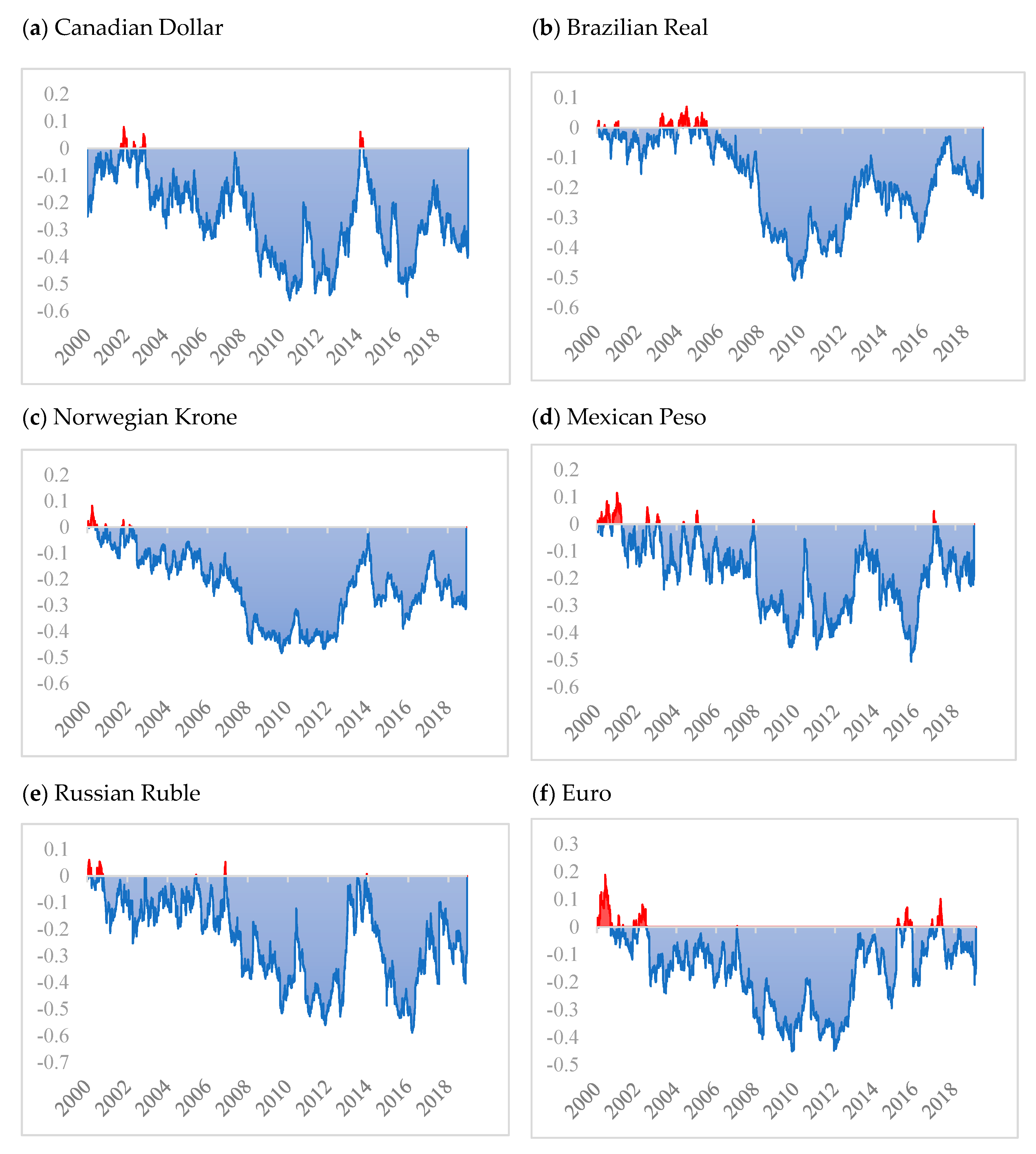
Figure 1 shows the results of dynamic correlation between WTI crude oil and the currency market using the ADCC-GARCH model. Results of the dynamic correlation between WTI oil and FX market highlight negative correlation values, except for the Japanese Yen. According to [10], there may exist many counterbalancing factors that may not allow the exchange rate countries to move in a similar direction with crude oil prices. The findings are also corroborated by the findings of [52], who find negative correlations between oil prices and exchange rates. Further, Indian rupee and Euro also highlight some positive correlation between the 2000–2002 period; however, afterward, it exhibits a negative correlation consistently with WTI crude oil. We also observe that the negative correlation for most of the currencies reaches its maximum values between 2010 and 2014 and then in 2016 except the Japanese Yen. In the case of the Japanese Yen, positive correlation dominates negative correlation and reaches its highest level of 0.3–0.4 across the sampling period. Such a positive correlation between Japanese Yen and crude oil can be a result of Japan being a high importer of crude oil [15]. These results are also highlighted in Table 2 under the safe-haven and hedging of the oil, where the Japanese Yen remains the only currency with which WTI crude oil exhibits neither hedging nor safe-haven properties. Therefore, a clear distinction between the weak and strong safe haven or hedging properties of oil with different currencies can help in protecting investors in gaining optimal returns.

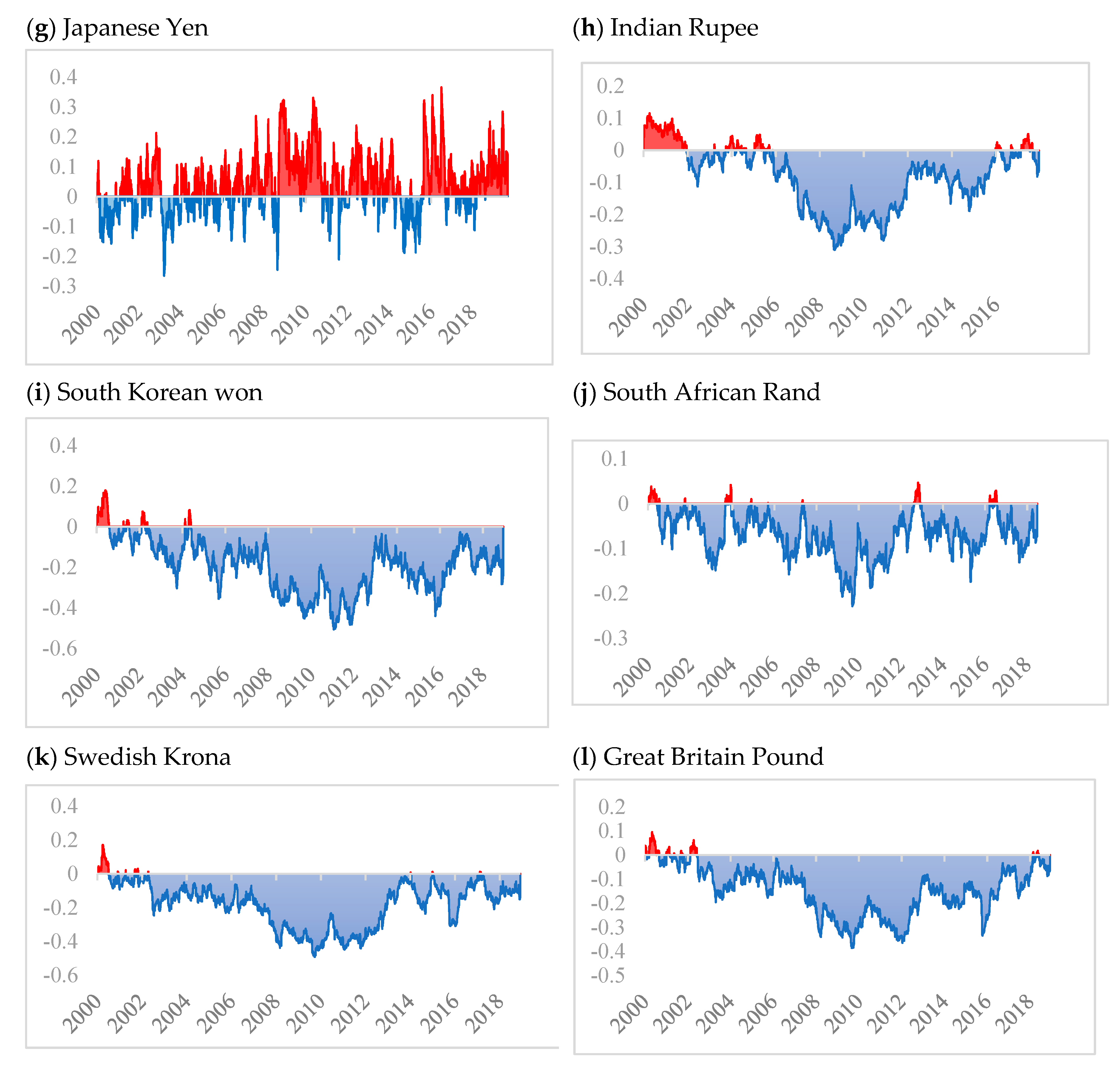
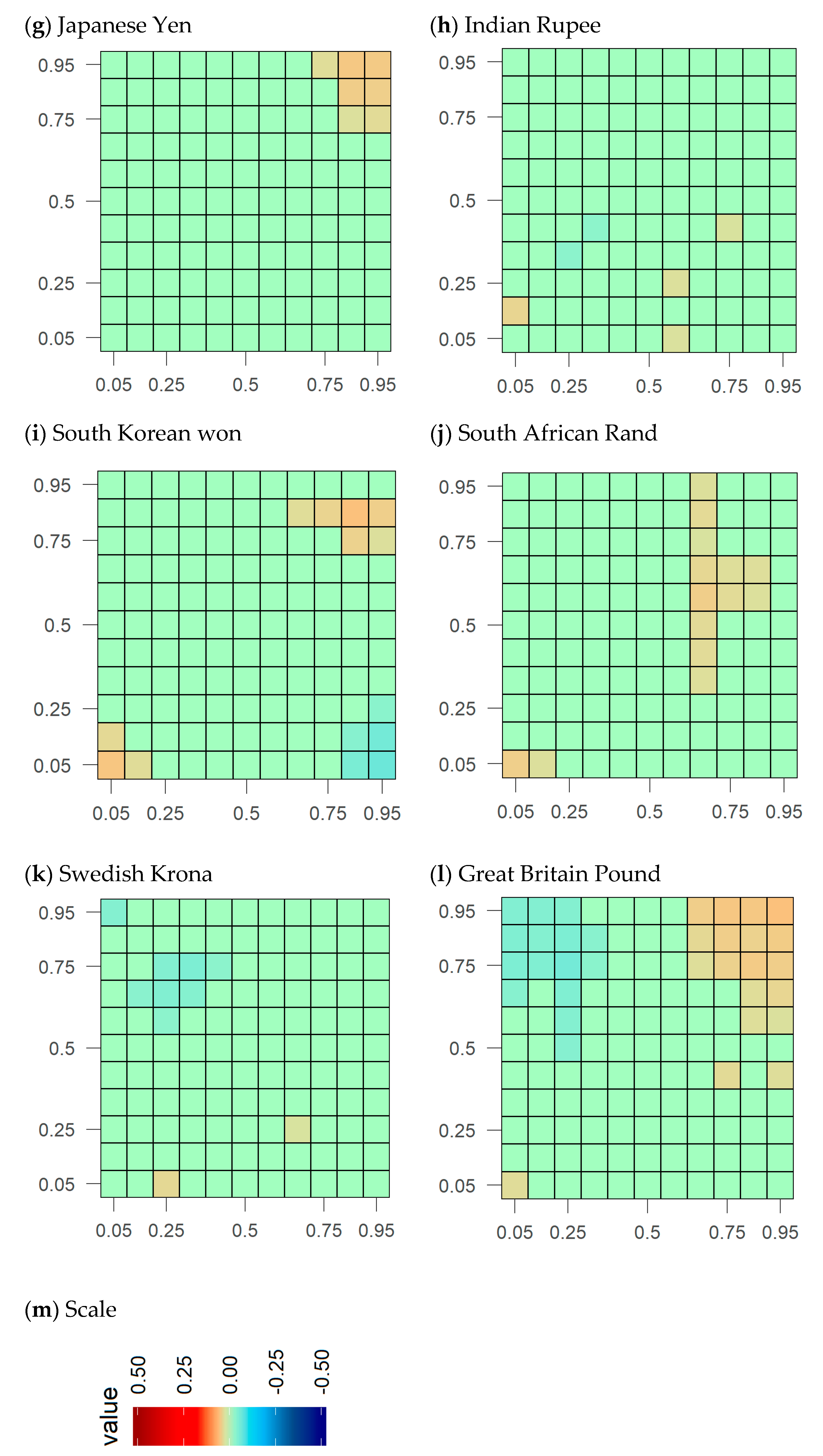
Figure 2 shows the results of the cross-quantilogram analysis between oil and currency market. We witness no significant dependence between oil and the FX market across the majority of the quantiles; however, few combinations of the significant coefficients are visible in the extreme quantiles of both oil and the FX market. Our results are corroborated by the findings of [53], that indicate that except Russia, returns correlation exists between the FX markets of BRICS countries with crude oil. The extreme positive returns in the WTI oil market are associated with the extreme positive returns in the FX markets of Russia, Japan, and South Korea. According to [2], the FX market of Russia is correlated with international crude oil prices. The extreme negative returns in the FX market of Norway and South Korea are followed by extreme negative returns in the oil market. Canadian dollar and GBP are the only markets for which the dependence on oil exists for both positive as well as extreme negative returns. Besides the aforementioned moderate dependence in the quantiles of oil and FX markets, we also witness strong traces in a few quantiles of both oil and FX markets. These traces are more evident for the Canadian dollar, Norwegian Krone, Euro, Swedish Krona, and the GBP, where extreme negative returns in these FX markets are associated with the extreme positive returns in the oil market. We also find an association between the extreme negative returns of Brazilian Real and Mexican Peso with extreme positive returns of oil futures; however, unlike the above-mentioned countries, dependence is evident only for few quantile arrangements. Some markets do not exhibit any strong dependence on the oil market, i.e., Russia, India, South Africa, Japan, and South Korea, in either of the quantiles. Therefore, these markets tend to act as safe-havens with oil in a portfolio. Therefore, these FX markets provide investors an opportunity to reduce their overall losses by moving against other oil futures during normal and crises periods. We witness strong safe haven properties of these FX markets (except Japanese yen) and therefore these FX markets have the potential to provide cover against losses together with oil futures in a portfolio when needed most.

Table 3. Summary statistics for hedge effectiveness (HE) and hedge ratio.

	Mean	Minimum	Maximum	HE
CAN	−0.0771	−0.1680	−0.0333	0.1516
BRA	−0.0829	−0.3266	−0.0086	0.0586
NOR	−0.0742	−0.1654	−0.0274	0.0845
MEX	−0.0784	−0.3006	0.0166	0.0735
RUS	−0.1241	−0.3068	−0.0289	0.1910
EUR	−0.0157	−0.0629	0.0480	0.0013
JPY	0.0194	−0.0685	0.1795	0.0193
IND	−0.0068	−0.0314	0.0096	0.0003
SKR	−0.0183	−0.0688	0.0100	0.0052
SAF	−0.1056	−0.3468	−0.0112	0.0639
SWE	−0.0355	−0.1141	0.0118	0.0167
GBP	−0.0401	−0.2791	0.0063	0.0356

Note: Fixed-window rolling analysis was used to calculate the hedge ratios in order to estimate the one step ahead forecast. Multivariate normal distribution was used for estimating the ADCC-GARCH estimates. For all specifications, a constant and an AR(1) term was included in the mean equation.

displays the results of hedging effectiveness and hedge ratio of WTI crude oil with each of the FX markets separately in a portfolio. Our results highlight that mean values are negative between oil and each of the FX markets except Japanese Yen. These negative average values imply an inverse association between currencies and oil prices and suggest that to take a hedge position, either a short or long position is to be taken for both assets, i.e., oil and either of the FX markets. For example, a long position of $1000 in Russian Ruble futures is hedged by taking another long position of $124 in the WTI oil futures. Likewise, a $1000 long position in Japanese Yen is to be hedged by taking a short position of $194 in the oil futures. However, we note significant variations in the mean values of different currencies, e.g., in case of the FX markets of Canada, Brazil, Norway, Mexico, Russia, and South African Rand, a higher amount of USD is required to hedge these currencies with the WTI oil futures. On the other hand, Indian Rupee Japanese Yen, Euro, South Korean Won, GBP, and Swedish Krona GBP require a low amount of USD for hedging with oil futures. It is also noteworthy that variance in the hedging values for the FX market of Brazil, Mexican, Russian, and South African Rand is high, implying high variance in the amount of USD required to hedge these currencies with oil.

Finally,

Table 4. Diversification benefits of oil for various portfolio compositions and probabilities.

	Panel A: at 5% Level					Panel B: at 50% Level
	0.05	0.20	0.50	0.80	0.95	0.05	0.20	0.50	0.80	0.95
CAN	0.0771	0.2768	0.5786	0.7457	0.5555	0.0168	0.0741	0.2278	0.3796	0.2067
	(0.0273)	(0.0786)	(0.1009)	(0.0548)	(0.0697)	(0.0063)	(0.0267)	(0.0697)	(0.065)	(0.0475)
BRA	0.113	0.3582	0.6369	0.6947	0.4264	0.0256	0.106	0.2714	0.3228	0.1362
	(0.046)	(0.0976)	(0.0841)	(0.0649)	(0.0967)	(0.012)	(0.041)	(0.0685)	(0.0643)	(0.0455)
NOR	0.0982	0.3313	0.6308	0.7325	0.4796	0.0218	0.0938	0.2658	0.3603	0.1602
	(0.0316)	(0.0788)	(0.0807)	(0.0397)	(0.0635)	(0.0077)	(0.0308)	(0.0675)	(0.0472)	(0.0353)
MEX	0.0835	0.2899	0.5817	0.7173	0.5042	0.0184	0.0795	0.23	0.344	0.1755
	(0.0353)	(0.09)	(0.0977)	(0.0463)	(0.0796)	(0.0085)	(0.0336)	(0.0715)	(0.0518)	(0.0445)
RUS	0.0758	0.2554	0.5109	0.6756	0.5658	0.0169	0.0726	0.2072	0.3198	0.2222
	(0.0542)	(0.1494)	(0.2047)	(0.1255)	(0.1198)	(0.013)	(0.0513)	(0.1207)	(0.1086)	(0.0778)
EUR	0.0768	0.2753	0.57	0.7143	0.503	0.0167	0.073	0.2183	0.3401	0.1732
	(0.024)	(0.067)	(0.0799)	(0.0431)	(0.0621)	(0.0056)	(0.0233)	(0.0571)	(0.0489)	(0.0369)
JPY	0.068	0.2465	0.5173	0.6445	0.4371	0.0147	0.0633	0.1818	0.2709	0.1395
	(0.0212)	(0.0586)	(0.0665)	(0.0415)	(0.0764)	(0.0049)	(0.0191)	(0.0384)	(0.0347)	(0.0384)
IND	0.0441	0.1674	0.3985	0.6181	0.5893	0.0094	0.0418	0.1319	0.2621	0.2328
	(0.0319)	(0.0986)	(0.1591)	(0.1184)	(0.0876)	(0.0073)	(0.0298)	(0.0748)	(0.0832)	(0.0585)
SKR	0.0641	0.2356	0.5132	0.6809	0.5103	0.0138	0.0604	0.1817	0.303	0.1791
	(0.0253)	(0.0713)	(0.0854)	(0.0267)	(0.0778)	(0.0059)	(0.0235)	(0.0508)	(0.0247)	(0.046)
SAF	0.1288	0.3975	0.6724	0.691	0.3924	0.0294	0.1215	0.3014	0.3161	0.1184
	(0.0387)	(0.0839)	(0.0708)	(0.0495)	(0.0716)	(0.0099)	(0.0367)	(0.0643)	(0.0503)	(0.0321)
SWE	0.0934	0.318	0.6127	0.7171	0.4705	0.0207	0.0889	0.2514	0.3423	0.1552
	(0.0315)	(0.0802)	(0.0837)	(0.0379)	(0.0625)	(0.0076)	(0.0306)	(0.068)	(0.0433)	(0.0342)
GBP	0.0738	0.2668	0.56	0.7124	0.5103	0.016	0.0701	0.2109	0.3368	0.1771
	(0.0234)	(0.0658)	(0.0793)	(0.0364)	(0.0591)	(0.0055)	(0.0224)	(0.0527)	(0.0401)	(0.0354)

Note: The table illustrates the conditional diversification benefit for portfolios composed of crude oil WTI and conventional currencies. We calculated the diversification benefit for the shortfall values at the 5% (Panel A) and 50% (Panel B) probability levels. For each portfolio the table displays the average and standard deviation of the conditional diversification benefit. The standard deviations are presented in ( ).

presents the diversification benefits of a portfolio between oil and each of the FX markets under extreme negative and median quantile distribution with several combinations of portfolio weights. Panel A of Table 4 presents CDB analysis at a 5% level, which represents the extreme left tail distribution of returns for both markets. It is interesting to note that the diversification benefits gradually increase with an increasing weightage of WTI oil in a portfolio and achieves an optimal level of diversification up to 80% of its proportion in a portfolio, after which the CDB declines. These results are similar and consistent for all the FX markets. It is also noteworthy that despite an increasing CDB value for Russian and Indian FX markets, results appear insignificant for all weightage combinations for Russia and 50% and 80% oil weightage in the Indian FX market. In terms of comparison among the FX markets, Brazil has the maximum CDB with oil in a portfolio compared with other FX markets. Panel B of Table 4 represents conditional diversification benefits for the oil and FX market in a portfolio under median returns distribution at 50%. We can see that like results in Panel A, CDB in Panel B for all the FX markets initially increase with an increasing proportion of oil in a portfolio and reaches its maximum level up to 80% of portfolio weightage, after which it decreases. In terms of the comparison of CDB results under 5% and 50% returns distribution, results under extreme negative returns distribution provides better diversification benefits which carry significant implication for investors when both markets experience bearish conditions. Finally, among all foreign currencies, South African Rand and Swedish Krona offer maximum conditional diversification benefits under median returns distribution at 50% across all combinations of portfolio weights.

5. Conclusions

From the global trade finance point view the oil–currency relationship is critical because whenever there is a significant movement in crude oil price or dollar value, this causes co-movement of major currency pairs widely used by oil-exporting and importing countries. Additionally, considering the financialization of oil market post-2000s and ever-increasing volatilities in the FX and crude oil market in the last decade, the understanding of the linkages between both markets have crucial implications for traders and regulators. Accordingly, investors and other market participants are always considering different risk management practices to reduce and diversify risks in both markets. Thus, unlike the conventional literature on currency–oil nexus, this study holds unique insights on currency–oil relationship. We explored the likelihood of utilizing WTI crude oil prices as a risk-hedging tool for conventional currencies. This study asked the question of whether crude oil prices can constitute as a hedge, safe-haven, and diversifier for conventional currencies. As both markets share various common drivers and informational dependencies, we explored whether taking offsetting positions across both markets offers market participants with effective hedging and diversification opportunities. We also examined the conditional diversification benefits of adding oil to currency portfolios. For the underlying objectives, we used several estimation techniques pertinent to our study objectives. More importantly, comparing the findings obtained from a variety of methods allowed us to better understand the dynamic linkages between crude oil and currency markets. In addition, the study used a sample of a broad range of major currencies including oil exporting and importing.

From the analysis employed in the study we learnt many things regarding the currency–oil nexus. First, the empirical evidence obtained from a broad range of currencies, including oil exporting and importing, shows that crude oil acts as a strong safe-haven and hedge for conventional currencies for most cases. Additionally, the findings from dynamic correlation analysis highlight that the time varying correlations between WTI oil and the currencies are mostly negative values. This is further corroborated by the evidence of hedging ratio and hedging effectiveness of WTI crude oil with sample currencies, which highlights that mean values are negative between oil and each of the FX markets except Japanese Yen. The inverse relationship between oil and currencies suggest taking a hedge position, either short or long position is to be taken for both assets, i.e., oil and either of the FX markets. The additional evidence from the cross-quantilogram analysis shows no significant dependence between oil and the FX market across the majority of the quantiles; however, few combinations of the significant coefficients are visible in the extreme quantiles of both oil and the FX market. Moreover, few markets, i.e., Russia, India, South Africa, Japan, and South Korea, do not show dependence with the oil market in either of the quantiles. This shows that the mentioned markets can serve as safe-havens with oil in a portfolio. Finally, the findings reveal including oil in currency portfolio assists in formulating more diversified and improved portfolio performance. In addition, diversification benefits of a portfolio between oil and currencies shows that conditional diversification benefit of the oil is higher in the lower quantiles, i.e., when both currency and oil markets are in a bearish state. Overall, the main take-away from this study is that crude oil prices hold strong hedging and safe-haven properties for major currencies and further crude oil prices can be effectively used as risk-hedging tools for currency appreciation and depreciation in both oil-exporting and importing countries.

Considering the increasing importance of crude oil for international trade finance and the evidence that suggests the functional role of crude oil in currency portfolio, the study highlights important policy implications for policymakers and traders. The findings are useful for central banks seeking to manage exchange-rates and oil inflation. More importantly, the findings are useful for the risk management of oil and related assets in oil-exporting and importing economies. Moreover, the findings can assist portfolio managers in taking better hedging strategies to limit the detrimental effects of volatility in the FX and crude oil markets. It is worth mentioning that although we maintain our findings are quite useful for portfolio managers and investors for risk management purposes, still, we also believe that many other related issues must also be addressed carefully. Especially, the role of policy regime shifts must be meticulously evaluated as the policy shocks may have significant influence on the future relationship between currencies and crude oil prices. Nevertheless, future research can use the insights of this study to formulate new hedging strategies for currencies using other energy and non-energy commodities. In particular, considering the growing stress on environmental awareness and renewable energy resources, future research can focus on exploring the dynamic linkages between major currencies and renewable resources. Investigations of this nature will assist market participants to make better risk management decisions in the future since renewable resources are considered to be more important in the future. Additionally, employing such strategies will allow market participants to take advantage of financialization of commodity markets for the risk management of FX portfolios.