Liquid-Liquid Flow Pattern Prediction Using Relevant Dimensionless Parameter Groups

Abstract

Accurate predictions of flow patterns in liquid-liquid flow are critical to the successful design and operation of industrial and geo-energy systems where two liquids are jointly transported. Unfortunately, there is no unified flow pattern map, because all published maps are based on limited ranges of dimensional parameters. Dimensional analysis was performed on oil-water horizontal flows, to obtain some relevant dimensionless parameter groups (DPG) for constructing flow pattern maps (FPM). The following combinations of DPG were used: (i) the ratio of mixture Reynolds number to Eötvös number versus water fraction, (ii) the ratio of Weber number to Eötvös number versus water fraction, (iii) the mixture Froude number versus water fraction, (iv) the water Froude number versus oil Froude number, (v) the ratio of gravity force to viscous force versus water fraction. From twelve published experimental studies, 2696 data points were gathered and analysed covering a variety of flow patterns including stratified, stratified mixed, dispersed oil in water, dispersed water in oil, annular and slug flows. Based on the performed analysis, it was found that flow patterns could occupy more than one isolated region on the DPG-based flow pattern map. None of the combinations of DPG can mark out all the considered flow patterns, however, some combinations of DPG are particularly suitable for marking out the regions associated with some flow patterns.

1. Introduction

Due to their applicability in various process industries, horizontal liquid-liquid flows have been extensively studied. Such research is particularly important in the energy sector, where oil and water are usually co-produced and transported jointly. However, despite the importance of liquid-liquid flows, they have not been studied to the same extent of the gas-liquid flows [1,2] and there is no unified flow pattern map for the liquid-liquid flows [3]. In most cases, the flow pattern maps available for the liquid-liquid flow are limited to the conditions for which the flow maps were constructed [4]. Figure 1 presents a liquid-liquid flow pattern map developed for mineral oil and tap water, featuring superficial phase velocities. Various other parameters have been employed in the construction of flow pattern maps, as discussed in Section 2.2. The use of dimensionless groups to develop flow pattern maps would lead to a wider range of applicability [5]. Therefore, this project focuses on the construction of flow pattern maps using various combinations of relevant dimensionless parameter groups to ensure wider usage in horizontal pipes.

The earliest research into liquid-liquid flow targeted the improvement of transportation of crude oil in pipelines [6,7,8,9], but liquid-liquid flow research is also important for flow in oil well production tubing, enhanced oil recovery (EOR) methods, and the design of chemical reactors and separators [10].

Figure 1. Graph of superficial water velocity versus superficial oil velocity modified after Trallero et al. [11] developed for an inner pipe diameter of 50.1 mm, with µ_o = 0.0288 Pa s, µ_w = 0.00097 Pa s, ρ_o = 884 kg/m³, ρ_w = 997 * kg/m³ and σ = 0.036 N/m at 25.5 °C. Note: for data with ⁽*⁾, the authors recorded 1037 kg/m³ for tap water at ≈25.5 °C.

Figure 1. Graph of superficial water velocity versus superficial oil velocity modified after Trallero et al. [11] developed for an inner pipe diameter of 50.1 mm, with µ_o = 0.0288 Pa s, µ_w = 0.00097 Pa s, ρ_o = 884 kg/m³, ρ_w = 997 * kg/m³ and σ = 0.036 N/m at 25.5 °C. Note: for data with ⁽*⁾, the authors recorded 1037 kg/m³ for tap water at ≈25.5 °C.

1.1. Importance of Flow Patterns in the Industrial Sector

Understanding the nature and behaviour of liquid-liquid flow is critically important but also challenging, as many physical and, sometimes, chemical mechanisms govern the formation of flow patterns. Once a flow pattern is determined, some key process parameters, such as pressure gradients and phase fractions of that particular flow system could be estimated.

In oil-water pipelines, stratified flow exists at low velocities with oil flowing at the top while water flows at the bottom in a horizontal pipe. The bottom section of the pipeline is prone to corrosion due to the continuous flow of water [12,13] and the dissolution of gases, such as CO₂ and H₂S in water, which are attributed as the cause of corrosion. The oil phase by itself is considered non-corrosive [14], so in theory, a pipeline which has no free-flowing water phase (i.e., the water phase is entirely entrained in the oil phase) is free of corrosion problems [13,15].

It is essential to determine the flow pattern for an optimal process of injecting inhibitors and other chemicals into the pipeline to prevent corrosion. Furthermore, predicting the flow pattern of a pipeline is essential for calculating the pressure drop along it, which improves design and optimises maintenance of the pipe itself.

At ambient conditions, viscous heavy oil does not flow easily. Before transporting such crude, its high viscosity is usually reduced, by either heating it, adding a diluent, or both. Charles et al. [7] and Shi et al. [16] found that the introduction of water into a heavy oil pipeline can reduce both the pressure gradient along it and the power required to pump a given amount of the crude. An ideal flow pattern for transporting heavy oil is the core-annular flow (CAF), where the crude flows in the core, while a small quantity/amount of water forms annulus around the oil and lubricates the pipeline [2,7,10,16]. The injected water is pre-treated with a demulsifying agent to help the phase separation at the end of the pipeline [17], so flow pattern determination can suggest the most appropriate way of transporting multiphase flow fluids.

There is a substantial difference in the pressure gradients encountered with various flow patterns [17]. For dispersed flows, a system of two immiscible fluids (oil and water) can become more complex as the resulting mixture fluid may become an emulsion, which is unstable when it separates into the original phases that formed it within a reasonable period of time at rest.

When designing an oil-water pipeline, an accurate prediction of the phase inversion point is desirable as there is a significant difference between the pressure drop in the oil-dominated and the water-dominated regions [17]. Phase inversion is a phenomenon in oil-water flow systems where the dispersed phase switches to be the continuous phase. With saline water, the inversion point can be observed earlier than with tap water (0.45 and 0.5 oil fraction for saline and tap water, respectively) [18]. At the inversion point, the oil-water mixture viscosity can increase dramatically, so pipeline operators strive to avoid operating at this flow condition [17]. This can be achieved with a good understanding of the system flow patterns.

1.2. Liquid-Liquid Flow Patterns in Horizontal Pipes

When two immiscible liquids flow together in a horizontal pipeline, different flow patterns are experienced. The factors responsible for the flow pattern configurations include density ratio, viscosity ratio, input phase ratio, mixture flow rate, wetting properties, surface tension and pipe geometry [2,19]. For example, using the same experimental facility, two different flow pattern descriptions were obtained by two researchers, who operated at the same conditions, but used two various working fluids [11]. The name given to a particular flow pattern may not always be meaningful as it does not describe the features of the flow pattern [11]. Various researchers have described the flow patterns with different names and terminologies, Section 2.3 resolves this challenge. In addition, the number of flow patterns reported for liquid-liquid horizontal pipes varies from one researcher to another with Oglesby [20], Trallero et al. [11], Nädler and Mewes [21], Brauner [2] and Al-Wahaibi et al. [22] reporting fourteen, six, seven, eighteen and six flow patterns, respectively. Figure 2, Figure 3 and Figure 4 present some of these flow patterns.

For an accurate prediction of the multiphase flow features, it is essential to identify the flow pattern, because uncertainties in flow pattern determination greatly affect the liquid-hold up and pressure drop predictions [23]. Therefore, the flow pattern is a defining feature of multiphase flow. In predicting local flow pattern, flow pattern maps are employed. A flow pattern map is generally a 2-D graph with transition boundaries which separate the graph into areas with similar flow configuration called flow pattern [24].

A literature review of two immiscible liquids flowing in the horizontal pipeline showed that there is no unified/standard flow pattern map for all investigators [3]. Different investigators have presented their flow pattern maps on various coordinates which makes the comparison and interpretation of the published flow patterns difficult [11]. A detailed discussion of the chronological development of flow pattern maps in Section 2.2. The application of flow pattern maps based on dimensional parameters is limited to the particular pipe size and fluids used for constructing them [4]. Flow pattern maps with a wider range of applicability can be achieved when relevant dimensionless parameters are used for constructing them [5].

2. Data Collection

The key aim of this study is to utilise relevant dimensionless parameters to develop more accurate flow pattern maps for liquid-liquid flow in horizontal pipes. As such, an important initial step is a thorough investigation into the relevant literature to scope suitable experimental studies and to create a pool of data points to allow meaningful trends to be observed. Theoretical studies have also been considered in this process as, although they do not contribute to the flow maps themselves, they provide valuable insight into the physical phenomena and allow a more informed set of flow maps to be developed.

As there are a number of geometric, flow conditions and fluid characteristics that may influence the flow pattern [19,25], a rigorous approach has been taken to ensure consistency between the experimental studies included in this study. The selected experimental studies were based largely on datasets accessibility, pipe inclination and flow conditions. The main criteria for inclusion are presented in

Table 1. Main conditions for including an experimental study.

Group of Factors	Factor	Criterion	Reasons
Pipe Geometry	Pipe inclination	Horizontal (0°)	This study focuses solely on horizontal flow, as pipe inclination influences the interaction between the dominant forces (inertial, gravity and buoyancy), which can delay or accelerate the emergence of a flow pattern [26]
	Pipe internal diameter	10–100 mm	So far most of the studies of multiphase pipe flows were conducted in the closed channels with a hydraulic diameter ranged from 10 mm to 100 mm. The multiphase flow behaviors in small diameter (<10 mm) pipes are significantly different from that in the pipes of conventional scales, as the Eötvös numbers in the small pipes are small hence the interfacial tension is critically significant in comparing to the gravitational forces. On the other hand, Cheng et al. [27] also showed that behaviors of multiphase flows in large diameter (>100 mm) pipes could be substantially different from that in smaller pipes
Fluid Properties	Density	Water (~1000 kg/m3), oil (750–900 kg/m3)	The buoyancy and gravity forces are direct function of density [26] At relatively low flow rate, high density difference between the two phases results in stratified flow [28,29,30] With equal density phases, no stratification [7]
	Viscosity	Water (0.8–1.0 mPa s), oil (<700 mPa s)	Interfacial instability increases as the difference in viscosity between the two phases increases [28]
	Interfacial tension	0.01–0.06 N/m	From moderate to relatively high velocities, interfacial instability is high due to high turbulence, which leads to faster transition from stratified to non-stratified flow [28]
Flow Conditions	Temperature	~25 °C	The operating temperature of an experimental set-up has a significant influence on the physical properties of the fluids [31]
	Pressure	~1 atm	Oil and water are usually treated as incompressible fluids, hence the pressure effect on physical properties of liquid-liquid flow is considered negligible [32]

.

This section provides an overview of the considered literature and also highlights the reasons for the inclusion of the experimental studies in the final data set. It should be noted that all reasonable efforts were made to acquire the experimental flow maps, but that this was not always possible if the data had not been presented or made available for download.

Finally, it can be noted that, while the intention of this section was not to create a literature review, sufficient detail has been included to provide a thorough overview of research in this area.

2.1. Experimental Studies on Liquid-Liquid Flow in Horizontal Pipelines

A summary of some relevant experimental works published on liquid-liquid flow in horizontal pipes is provided in Table 2. The pipe diameters vary from 5.6 mm to 101.2 mm, with the majority ranging from 19 mm to 30 mm, and just two experimental works having pipe diameters less than 19 mm [33,34]. Only a few of the experimental studies used pipe diameters greater than 60 mm [35,36,37]. The ratios of oil to water viscosity and density range from 0.7 ≤ µ_o/µ_w ≤ 12550, and 0.684 ≤ ρ_o/ρ_w ≤ 1, respectively, whilst the interfacial tension (σ) ranges from 0.017 N/m to 0.05 N/m.

Determination of flow pattern is the key to modelling of liquid-liquid flow as all of the design variables are dependent on the flow pattern, e.g., the pressure drop of oil-water flow in a horizontal pipeline depends on the flow pattern [6,7,17,21,38,39]. Experimental studies relevant to this project that have been performed to determine flow patterns in oil-water horizontal flow are presented chronologically in Table 2.

The data provides an idea about the pipe roughness and wettability, which influence the pressure gradient, flow patterns and the hold-up. Angeli and Hewitt [30] observed that flow patterns were more disturbed in steel pipes than in acrylic pipe, which explained why there was a very small stratified wavy region and the mixed region began at lesser velocities in the former.

Recent studies on liquid-liquid flow have focused more on high viscous oil-water flow due to its relevance to the petroleum industry activities enhanced oil recovery (EOR) and heavy oil transportation [40]. Annular flow, a flow pattern associated with the highly viscous oil-water flow system, is more pronounced in those studies where high viscosity oil is used [41,42,43]. Detailed studies of the annular flow pattern are necessary to reduce the head-loss due to high oil viscosity during transportation [40,44]. Charles et al. [7] suggested that high and low viscosity oils behave differently due to their wall wetting effects. Note that oil viscosity is classified into <10 mPa s, 20–100 mPa s and >100 mPa s as low-viscous oil, medium-viscous oil and heavy-viscous oil, respectively [3,45].

Where there is a small density difference (Δρ) between the two liquids for a liquid-liquid flow system, the effect of gravitational forces is reduced. The wetting ability and interfacial tension properties of liquids have a significant impact on the flow patterns [10,15]. When two immiscible liquids flow together in a pipe, they tend to stratify, but the higher the density difference (Δρ) is, the better is the achieved stratification [7].

Interfacial tension and the gravity forces tend to stabilise the interface between the layers of two immiscible liquids. Yet when these stabilising forces are less than the destabilising forces (relative movement and the viscosity difference between the two liquids, the interface becomes destabilised [22,28,46]. High interfacial tension between the two liquids will prevent the growth of amplitude at the interface and thereby stabilise the interface.

There have been significant developments in flow patterns detection over the years. The measuring techniques range from simple to more sophisticated techniques such as visual observation, photography (video-camera), high-frequency impedance probe, conductivity needle probe, particle image velocimetry, dual impedance probe, and hot-wire anemometry.

As discussed in Section 1.2, density ratio, viscosity ratio, input phase ratio, mixture flow rate, wetting properties, surface tension and pipe geometry are factors influencing the flow patterns [2].

Wang and Gong [47] showed the differences between high viscosity mineral oil-water flow and crude oil-water flow in horizontal pipelines, commenting that mineral oil was more widely used than the crude oil in the liquid-liquid flow experimental studies. Even where both mineral and crude oils had approximately the same viscosity and density, they found out that their flow patterns and transition boundaries did not agree. In terms of similarity, they observed that the flow patterns of both mineral oil-water and crude oil-water flow systems could be grouped into oil-dominated, water-dominated, intermittent, and stratified regions. The presence of some natural surfactants or depositions in crude oil, such as resin and asphaltenes caused a delay in the transition from one flow pattern to another [40,48].

The choice of mixing device is essential in the experimental studies, as each device promotes the formation of a particular flow pattern. An injecting device promotes core-annular flow [40] whereas cones or special “Y” mixing devices support stratification of flow to avoid mixing [25].

Table 2. Experimental works on oil-water flow patterns in horizontal pipelines.

Author	Year	Diameter (mm)	Pipe Material	µo/µw	ρo/ρw	σ (mN/m)	Velocity Range (m/s)	Measurement Techniques	Observed Flow Patterns	Fluids Used	Temperature/Pressure	Mixing Device	L/D
Russell et al. [6]	1959	20.5	Cellulose acetate butyrate	20.13	0.834	40	vso = 0.01–1.0, vsw = 0.04–1.08	VO + P (4 × 5 in Linhoof press camera with a 90 mm lens)	Bb, ST, mixed	Mineral oil-Kremol 70/water	25 °C/NP	48° Y	419
Charles et al. [7]	1961	26.4	Cellulose acetate butyrate	7.04, 18.79, 72.71	1	45, 45, 30	vso = 0.02–0.9, vsw = 0.043–1.07, 0.043–1.08, 0.043–1.09	VO + P	SL, AN, Bb, Dw/o, Do/w	Oil (Marcol CX)/water; Oil (Wyrol J)/water; Oil (Teresso 85)/water	25 °C/NP	Oil via nozzle, water via annulus	277
Hasson et al. [33]	1970	12.6	Glass-pipe	1.22	ρm = 1020 kg/m3	17–17.5		VO + P	D, SL, ST, AN and mixed flows	Kerosene-perchloroethylene/distilled water	30 °C/NP	Inlet nozzle device for concentric flow	214
Guzhov et al. [38] Source: [49,50]	1973	39.4	Steel	21.8	0.896	44.8	vm = 0.3–1.6	VO	ST, ST & MI, Do/w, Dw/o, Do/w & w, Dw/o & o/w	NP	21°C/NP	NP	NP
Oglesby [20]	1979	41	Steel	167, 61, 32	0.87; 0.863; 0.859	35.4	NP	VO	ST, ST & MI, Do/w & w, o/w, Dw/o & Do/w, w/o, SL, SLw, AN, AO	Oil (Sun Oil Co. solvent (250-SN)/water; Oil (diesel fuel)/water; Oil (blend of Sun Oil Co. solvent (250-SN and diesel fuel)/water	NP; 18.3 °C/NP; 21.1 °C/NP.	90° angle 2 in T	282
Arirachakaran et al. [17]	1989	41	Steel	27.9, 344, 498, 682	0.854, 0.868, 0.868, 0.868	NP, 29, 30, 31	vm = 0.457–3.66	NP	ST, Do/w & w, o/w, o & Dw/o, w/o, SL, SLw, AN, AO	No. 2 Diesel fuel oil/tap water, Experimental oil No. 1/tap water, Experimental oil No. 2/tap water, Experimental oil No. 3/tap water	21.1 °C/NP	NP	312
Arirachakaran et al. [17]	1989	26.6	Steel	1405, 12550	0.869, 0.90	32, 32	vm = 1.5−3.05	NP	ST, Do/w & w, o/w, o & Dw/o, w/o, SL, SLw, AN, AO	Refined oil (SN-250)/tap water Refined oil (150-SB)/tap water	21.1 °C/NP	NP	229
Kurban et al. [51]	1995	24.3; 24	Glass, Acrylic	1.6	0.803	NP	NP	P + conductivity probe	ST, ST & MI, Dw/o	NP	NP	NP	NP
Trallero et al. [11]	1997	50.1	Acrylic resin	29.7	0.852	36	vso = 0.01–1.61, vsw = 0.01–1.83	VO	ST, ST & MI, Do/w & w, o/w, Dw/o & Do/w, o/w	Mineral oil (Crystex AF-M)/tap water	25.5 °C/NP	Y-type	310
Nädler and Mewes [21]	1997	59	Perspex	22–35	0.848	NP	vm = 0.3–1.61	VO + conductance probe	ST, ST & MI, Do/w & w, o/w, Dw/o & Do/w & w, Dw/o & w, w/o.	Mineral white oil (Shell Ondina 17)/tap water	30 °C, 25 °C, 18 °C/NP	Cone-shaped nozzle separated by baffle plates	225, 680
Vedapuri, et al. [36]	1997	101.6	Plexiglass	2; 90		NP	vm = 0.1–2.0	VO (by video home system camera)	ST & MI, Dw/o & o/w	Oil (Standard ASTM salt-water)/water	40 °C/0.13 MPa	T-junction	177
Valle and Utvik [35]	1997	77.9	Steel	1	0.741	NP	vm = 1.17, 1.74, 2.33	Conductivity needle probe	Do/w, Dw/o, S	Light crude oil/synthetic formation water	70 °C/10.5 MPa	NP	154
Bannwart [43]	1998	22.5	Glass	2700	0.989	40	vso = 0.30–0.63, vsw = 0.03–0.28	P (Kodak EktaPro EM high speed camera)	AN	Viscous oil/water	RT/NP	Nozzle (tube for oil, shell for water)	NP
Soleimani [52]	1999	25.4	Steel	1.6	0.801	17 @ 22 °C	vm = 1.25–3.0	VO, Impedance probe, Gamma densitometer	ST, SWD, SMW, SMO, 3L, Dw/o & Do/w	Kerosene/(Exxsol D80)/tap water	25 °C/NP	Static mixer	382
Angeli and Hewitt [30]	2000	24.3; 24	Steel; Acrylic resin	1.6	0.801	17	vm = 0.2–3.9	VO, high-speed video-camera, HFI probe	SW, SWD, SMO, 3L, SMW, Mixed	Kerosene (Exxsol D80)/tap water	20 °C/NP	T-junction	370; 375
Simmons and Azzopardi [37]	2001	63	PVC	1.125	0.684	10	vm = 0.8–3.1	Lasentec TM Par-Tec 300 C, Malvern 2600	SM, Dw/o & w, Dw/o	Kerosene/Aqueous potassium carbonate solution	NP	Mixer with porous walls	71
Mu [53] Source: [54]	2001	25.4	Steel	310	0.93	NP	NP	High-speed P	ST, ST & MI, SLw, AO Do/w, Dw/o	NP	NP	NP	NP
Bannwart et al. [42]	2004	28.4	Glass	488.0	0.926	29	vso = 0.007–2.5; vsw = 0.04–0.5	P (high speed camera (Olympus, 1000 frames/s) (at slow motion 30 frames/s))	ST, Bb, AN	Heavy crude oil/water	20 °C/NP	Injection nozzle (central tube for oil, shell for water)	191
Lovick and Angeli [55]	2004	38	Stainless steel	6.0	0.828	39.6	vm = 0.8–3.0	VO, conductance probe and HFI probe	SW, Dw/o, Do/w, DC	Mineral oil (ExxsolD140)/tap water	NP	T (mixing reduction)	210
Chakrabarti et al. [56]	2005	25.4	Polymethyl-methacrylate	0.7	0.787	45	vso = 0.029–2.12; vsw = 0.04–1.46	VO + P	ST, ST & MI, PL, Do/w & w, Dw/o & o	Kerosene/water	25 °C/NP	Mixer (pipe inserted in another pipe)	84
Wegmann and Rudolf von Rohr [34]	2006	5.6; 7	Glass	5.78–6.14	0.82–0.822	62.2 @ 20 °C	vso = 0.01–2.5, vsw = 0.01–2.0, vso = 0.01–1.6, vsw = 0.01–13.	P (digital camera (Minolta Dimage 7i with a resolution of 2560–1920 pixels)	ST, AN, I, Do/w, Dw/o	Paraffin-oil/water	19.1–23.3 °C/NP	T-shaped (selected to prevent emulsion formation	660; 528
Vielma et al. [57]	2007	50.8	Acrylic resin	18.8	0.859	16.4	vso = 0.03–1.75, vsw = 0.03–1.75	VO, P and conductance probe	ST, ST & MI, Do/w & w, o/w, Dw/o & Do/w, o/w	Refined mineral oil (Tulco Tech 80)/tap water	40 °C–29 °C/NP	30° Y	440
Grassi et al. [41]	2008	21	Polycarbonate	615	0.886	50	vso = 0.029–0.7, vsw = 0.14–2.5	VO + P	ST, Do/w, AN, PL/SL, Do/w & w	Paraffin oil/water	20 °C/NP	Injecting device (oil at the core and water annulus)	429
Dasari et al. [58]	2013	25	Perspex	107	0.889	24	vso = 0.015–1.22, vsw = 0.1–1.1	VO + P (camera model no DSC-HX100 V, by sony)	SL, ST, ST & MI, Do/w, Dw/o, PL	Lube oil/water	25 °C/NP	NP	40
Al-Wahaibi et al. [22]	2014	19	Acrylic	12	0.877	20.1	vso = 0.06–1.69,vsw = 0.12–1.69	VO + High speed camera (Fastec Troubleshooter, records up to 1000 fps)	ST, Bb, AN, DC, Do/w, Dw/o	Mineral oil/water	NP	Y-junction	421
Voulgaropoulos et al. [59]	2016	37	Acrylic	6.2	0.830	32.9	vm = 0.31–0.73	High-speed camera (with Tokina Macro lens) and a dual conductance probe	ST, SM, Do/w, Dw/o, Do/w & w, Dw/o & o/w	Kerosene (Exxsol D140)/fresh water	20 °C/NP	Multi-nozzle inlet	189

Note: v_so = Superficial oil velocity, v_sw = Superficial water velocity, v_m = Mixture velocity, VO = Visual Observation, P = Photography, HFI = High-frequency impedance, NP = Not provided L/D = the ratio of part of the test section in which testing actual took place or the length of the test section from entrance to inner diameter of the pipe, RT = room temperature, ρ_m = mixture density, µ_o/µ_w = ratio of oil viscosity to water viscosity, ρ_o/ρ_w = ratio of oil density to water density. Note: 3L:Three layers; AN: Annular/oil in water concentric; AO: Annular/oil annulus; Bb: Oil bubbles in water; D: Dispersed flow; DC: Dual continuous; Do/w: Dispersed oil in water; Dw/o: Dispersed water in oil; Do/w & w: Dispersion of oil in water with water layer; Dw/o & Do/w: Dispersed water-in-oil and oil-in-water; Dw/o & Do/w & w: Dispersed water in oil and dispersed oil in water, and water layer; I: Intermediate flow; M: Mixed; o/w: Oil-in-water emulsion; O & W/O: Oil layer and dispersed water in oil; PL: Plug flow; SL: Oil slugs in water; SLw: Water slugs in oil; SMO: Stratified mixed/oil; ST: Stratified flow; ST & MI: Stratified flow with mixing at the interface; SW: Stratified wavy; SWD: Stratified wavy with droplets at the interface (Stratified wavy/drops); SMW: Stratified mixed/water; w/o: Water-in-oil emulsion.

Table 2. Experimental works on oil-water flow patterns in horizontal pipelines.

Author	Year	Diameter (mm)	Pipe Material	µo/µw	ρo/ρw	σ (mN/m)	Velocity Range (m/s)	Measurement Techniques	Observed Flow Patterns	Fluids Used	Temperature/Pressure	Mixing Device	L/D
Russell et al. [6]	1959	20.5	Cellulose acetate butyrate	20.13	0.834	40	vso = 0.01–1.0, vsw = 0.04–1.08	VO + P (4 × 5 in Linhoof press camera with a 90 mm lens)	Bb, ST, mixed	Mineral oil-Kremol 70/water	25 °C/NP	48° Y	419
Charles et al. [7]	1961	26.4	Cellulose acetate butyrate	7.04, 18.79, 72.71	1	45, 45, 30	vso = 0.02–0.9, vsw = 0.043–1.07, 0.043–1.08, 0.043–1.09	VO + P	SL, AN, Bb, Dw/o, Do/w	Oil (Marcol CX)/water; Oil (Wyrol J)/water; Oil (Teresso 85)/water	25 °C/NP	Oil via nozzle, water via annulus	277
Hasson et al. [33]	1970	12.6	Glass-pipe	1.22	ρm = 1020 kg/m3	17–17.5		VO + P	D, SL, ST, AN and mixed flows	Kerosene-perchloroethylene/distilled water	30 °C/NP	Inlet nozzle device for concentric flow	214
Guzhov et al. [38] Source: [49,50]	1973	39.4	Steel	21.8	0.896	44.8	vm = 0.3–1.6	VO	ST, ST & MI, Do/w, Dw/o, Do/w & w, Dw/o & o/w	NP	21°C/NP	NP	NP
Oglesby [20]	1979	41	Steel	167, 61, 32	0.87; 0.863; 0.859	35.4	NP	VO	ST, ST & MI, Do/w & w, o/w, Dw/o & Do/w, w/o, SL, SLw, AN, AO	Oil (Sun Oil Co. solvent (250-SN)/water; Oil (diesel fuel)/water; Oil (blend of Sun Oil Co. solvent (250-SN and diesel fuel)/water	NP; 18.3 °C/NP; 21.1 °C/NP.	90° angle 2 in T	282
Arirachakaran et al. [17]	1989	41	Steel	27.9, 344, 498, 682	0.854, 0.868, 0.868, 0.868	NP, 29, 30, 31	vm = 0.457–3.66	NP	ST, Do/w & w, o/w, o & Dw/o, w/o, SL, SLw, AN, AO	No. 2 Diesel fuel oil/tap water, Experimental oil No. 1/tap water, Experimental oil No. 2/tap water, Experimental oil No. 3/tap water	21.1 °C/NP	NP	312
Arirachakaran et al. [17]	1989	26.6	Steel	1405, 12550	0.869, 0.90	32, 32	vm = 1.5−3.05	NP	ST, Do/w & w, o/w, o & Dw/o, w/o, SL, SLw, AN, AO	Refined oil (SN-250)/tap water Refined oil (150-SB)/tap water	21.1 °C/NP	NP	229
Kurban et al. [51]	1995	24.3; 24	Glass, Acrylic	1.6	0.803	NP	NP	P + conductivity probe	ST, ST & MI, Dw/o	NP	NP	NP	NP
Trallero et al. [11]	1997	50.1	Acrylic resin	29.7	0.852	36	vso = 0.01–1.61, vsw = 0.01–1.83	VO	ST, ST & MI, Do/w & w, o/w, Dw/o & Do/w, o/w	Mineral oil (Crystex AF-M)/tap water	25.5 °C/NP	Y-type	310
Nädler and Mewes [21]	1997	59	Perspex	22–35	0.848	NP	vm = 0.3–1.61	VO + conductance probe	ST, ST & MI, Do/w & w, o/w, Dw/o & Do/w & w, Dw/o & w, w/o.	Mineral white oil (Shell Ondina 17)/tap water	30 °C, 25 °C, 18 °C/NP	Cone-shaped nozzle separated by baffle plates	225, 680
Vedapuri, et al. [36]	1997	101.6	Plexiglass	2; 90		NP	vm = 0.1–2.0	VO (by video home system camera)	ST & MI, Dw/o & o/w	Oil (Standard ASTM salt-water)/water	40 °C/0.13 MPa	T-junction	177
Valle and Utvik [35]	1997	77.9	Steel	1	0.741	NP	vm = 1.17, 1.74, 2.33	Conductivity needle probe	Do/w, Dw/o, S	Light crude oil/synthetic formation water	70 °C/10.5 MPa	NP	154
Bannwart [43]	1998	22.5	Glass	2700	0.989	40	vso = 0.30–0.63, vsw = 0.03–0.28	P (Kodak EktaPro EM high speed camera)	AN	Viscous oil/water	RT/NP	Nozzle (tube for oil, shell for water)	NP
Soleimani [52]	1999	25.4	Steel	1.6	0.801	17 @ 22 °C	vm = 1.25–3.0	VO, Impedance probe, Gamma densitometer	ST, SWD, SMW, SMO, 3L, Dw/o & Do/w	Kerosene/(Exxsol D80)/tap water	25 °C/NP	Static mixer	382
Angeli and Hewitt [30]	2000	24.3; 24	Steel; Acrylic resin	1.6	0.801	17	vm = 0.2–3.9	VO, high-speed video-camera, HFI probe	SW, SWD, SMO, 3L, SMW, Mixed	Kerosene (Exxsol D80)/tap water	20 °C/NP	T-junction	370; 375
Simmons and Azzopardi [37]	2001	63	PVC	1.125	0.684	10	vm = 0.8–3.1	Lasentec TM Par-Tec 300 C, Malvern 2600	SM, Dw/o & w, Dw/o	Kerosene/Aqueous potassium carbonate solution	NP	Mixer with porous walls	71
Mu [53] Source: [54]	2001	25.4	Steel	310	0.93	NP	NP	High-speed P	ST, ST & MI, SLw, AO Do/w, Dw/o	NP	NP	NP	NP
Bannwart et al. [42]	2004	28.4	Glass	488.0	0.926	29	vso = 0.007–2.5; vsw = 0.04–0.5	P (high speed camera (Olympus, 1000 frames/s) (at slow motion 30 frames/s))	ST, Bb, AN	Heavy crude oil/water	20 °C/NP	Injection nozzle (central tube for oil, shell for water)	191
Lovick and Angeli [55]	2004	38	Stainless steel	6.0	0.828	39.6	vm = 0.8–3.0	VO, conductance probe and HFI probe	SW, Dw/o, Do/w, DC	Mineral oil (ExxsolD140)/tap water	NP	T (mixing reduction)	210
Chakrabarti et al. [56]	2005	25.4	Polymethyl-methacrylate	0.7	0.787	45	vso = 0.029–2.12; vsw = 0.04–1.46	VO + P	ST, ST & MI, PL, Do/w & w, Dw/o & o	Kerosene/water	25 °C/NP	Mixer (pipe inserted in another pipe)	84
Wegmann and Rudolf von Rohr [34]	2006	5.6; 7	Glass	5.78–6.14	0.82–0.822	62.2 @ 20 °C	vso = 0.01–2.5, vsw = 0.01–2.0, vso = 0.01–1.6, vsw = 0.01–13.	P (digital camera (Minolta Dimage 7i with a resolution of 2560–1920 pixels)	ST, AN, I, Do/w, Dw/o	Paraffin-oil/water	19.1–23.3 °C/NP	T-shaped (selected to prevent emulsion formation	660; 528
Vielma et al. [57]	2007	50.8	Acrylic resin	18.8	0.859	16.4	vso = 0.03–1.75, vsw = 0.03–1.75	VO, P and conductance probe	ST, ST & MI, Do/w & w, o/w, Dw/o & Do/w, o/w	Refined mineral oil (Tulco Tech 80)/tap water	40 °C–29 °C/NP	30° Y	440
Grassi et al. [41]	2008	21	Polycarbonate	615	0.886	50	vso = 0.029–0.7, vsw = 0.14–2.5	VO + P	ST, Do/w, AN, PL/SL, Do/w & w	Paraffin oil/water	20 °C/NP	Injecting device (oil at the core and water annulus)	429
Dasari et al. [58]	2013	25	Perspex	107	0.889	24	vso = 0.015–1.22, vsw = 0.1–1.1	VO + P (camera model no DSC-HX100 V, by sony)	SL, ST, ST & MI, Do/w, Dw/o, PL	Lube oil/water	25 °C/NP	NP	40
Al-Wahaibi et al. [22]	2014	19	Acrylic	12	0.877	20.1	vso = 0.06–1.69,vsw = 0.12–1.69	VO + High speed camera (Fastec Troubleshooter, records up to 1000 fps)	ST, Bb, AN, DC, Do/w, Dw/o	Mineral oil/water	NP	Y-junction	421
Voulgaropoulos et al. [59]	2016	37	Acrylic	6.2	0.830	32.9	vm = 0.31–0.73	High-speed camera (with Tokina Macro lens) and a dual conductance probe	ST, SM, Do/w, Dw/o, Do/w & w, Dw/o & o/w	Kerosene (Exxsol D140)/fresh water	20 °C/NP	Multi-nozzle inlet	189

Note: v_so = Superficial oil velocity, v_sw = Superficial water velocity, v_m = Mixture velocity, VO = Visual Observation, P = Photography, HFI = High-frequency impedance, NP = Not provided L/D = the ratio of part of the test section in which testing actual took place or the length of the test section from entrance to inner diameter of the pipe, RT = room temperature, ρ_m = mixture density, µ_o/µ_w = ratio of oil viscosity to water viscosity, ρ_o/ρ_w = ratio of oil density to water density. Note: 3L:Three layers; AN: Annular/oil in water concentric; AO: Annular/oil annulus; Bb: Oil bubbles in water; D: Dispersed flow; DC: Dual continuous; Do/w: Dispersed oil in water; Dw/o: Dispersed water in oil; Do/w & w: Dispersion of oil in water with water layer; Dw/o & Do/w: Dispersed water-in-oil and oil-in-water; Dw/o & Do/w & w: Dispersed water in oil and dispersed oil in water, and water layer; I: Intermediate flow; M: Mixed; o/w: Oil-in-water emulsion; O & W/O: Oil layer and dispersed water in oil; PL: Plug flow; SL: Oil slugs in water; SLw: Water slugs in oil; SMO: Stratified mixed/oil; ST: Stratified flow; ST & MI: Stratified flow with mixing at the interface; SW: Stratified wavy; SWD: Stratified wavy with droplets at the interface (Stratified wavy/drops); SMW: Stratified mixed/water; w/o: Water-in-oil emulsion.

A dimensionless length (L/D) is defined as the ratio of the length of the pipeline from the entrance to the observation point (sometimes equal to the length of the test section) to the pipe diameter. The L/D is a critical parameter for guaranteeing fully developed flow conditions [25].

Mukhaimer et al. [18] showed the effect of water salinity on flow patterns in an oil-water horizontal pipeline. They achieved water salinity of 75‰ by adding common salt (9% water weight) to the water tank. Due to this addition of salt, water density changed from 999 kg/m³ to 1065 kg/m³, while viscosity changed from 0.985 mPa s to 1.246 mPa s at 23.5 °C. Within a velocity range of 0.05–3 m/s for oil-tap water flow, seven flow patterns were observed, including: dispersed oil in water (Do/w), dispersed oil in water with water layer (Do/w & w), dispersed water in oil (Dw/o), dispersed water in oil and dispersed oil in water (Dw/o & o/w), stratified (ST), stratified with mixing at interface (ST & MI), and dispersed water in oil with oil layer (Dw/o & o). For the same velocity range, Dw/o & o was not observed with oil-saline water flow. They also observed that salinity delayed the transition from Do/w & w to Dw/o & o.

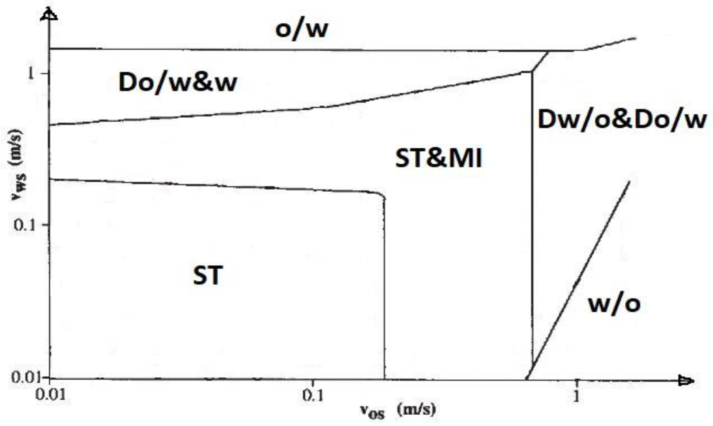
2.2. Development of Flow Maps for Liquid-Liquid in a Horizontal Pipeline

Various researchers have constructed flow maps for liquid-liquid flow in horizontal pipelines in several ways.

Table 3. Development of flow maps for liquid-liquid in a horizontal pipeline.

Author	Year	Mapping Parameters	Identified Flow Pattern
Russell et al. [6]	1959	Friction factor (ff) versus superficial water velocity (vsw)	Bb, ST, mixed
Charles et al. [7]	1961	Superficial oil velocity (vso) versus superficial water velocity (vsw)	w/o, AN, SL, Bb, and o/w
Hasson et al. [33]	1970	The organic phase flow rate (Qor) versus the water phase flow rate (Qw)	D, SL, ST, AN and mixed flows
Guzhov et al. [38] Source: [49,50]	1973	Mixture velocity (vm) versus input water fraction (fw)	ST, ST & MI, Do/w, Dw/o, Do/w & w, Dw/o & o/w
Oglesby [20]	1979	Mixture velocity (vm) versus input water fraction (fw)	ST, ST & MI, Do/w & w, o/w, Dw/o & Do/w, w/o, SL, SLw, AN, AO
Arirachakaran et al. [17]	1989	Mixture velocity (vm) versus input water fraction (fw)	ST, Do/w & w, o/w, o & Dw/o, w/o, SL, SLw, AN, AO
Vedapuri et al. [36]	1997	The thickness of the water layer to the diameter of the pipe, h/D against the percentage of water (input water fraction fw)	Semi-segregated, semi-mixed and semi-dispersed
Trallero et al. [11]	1997	Superficial water velocity (vsw) versus superficial oil velocity (vso) Mixture velocity (vm) versus input water fraction (fw)	ST, ST & MI, Do/w & w, o/w, Dw/o & Do/w, o/w
Nädler and Mewes [21]	1997	Superficial oil velocity (vso) versus superficial water velocity (vsw) Mixture velocity (vm) versus input water fraction (fw)	ST, ST & MI, Do/w & w, o/w, Dw/o & Do/w & w, Dw/o & w, w/o
Angeli and Hewitt [30]	2000	Mixture velocity (vm) against input water volume fraction (fw)	SW, SWD, SMO, 3L, SMW, Mixed
Brauner [2]	2003	(No map proposed) Eotvös number	Gravity force dominated or interfacial force dominated
Lovick and Angeli [55]	2004	Mixture velocity (vm) against input oil volume fraction (fo)	Dw/o, Do/w, DC, SW
Chakrabarti et al. [56]	2005	Superficial water velocity (vsw) versus superficial oil velocity (vso)	ST, SW, 3L, Do/w & w, D, PL, O & W/O
Wegmann and Rudolf von Rohr [34]	2006	Mixture velocity (vm) against input water volume fraction (fw)	ST, AN, I, Do/w, Dw/o
Vielma et al. [57]	2007	Superficial water velocity (vsw) versus superficial oil velocity (vso)	ST, ST & MI, Do/w & w, o/w, Dw/o & Do/w, o/w
Grassi et al. [41]		Superficial water velocity (vsw) versus superficial oil velocity (vso)	ST, Do/w, AN, PL/SL, Do/w & w
Hapanowic [60]	2010	Superficial mass fluxes for oil (gol,o) [kg/m2.s] versus Superficial mass fluxes for water (gw,o) [kg/m2.s]	Dr-drops, DrP-drops and plugs, D-dispersion, S-stratification AD-annular and dispersion; -W-for water, -O-for oil
Yusuf et al. [29]	2012	Superficial water velocity (vsw) versus superficial oil velocity (vso)	ST, Bb, AN, DC, Do/w, Dw/o
Dasari et al. [58]	2013	Superficial water velocity (vsw) versus superficial oil velocity (vso)	SL, ST, ST & MI, Do/w, Dw/o, PL
Al-Wahaibi et al. [22]	2014	Superficial water velocity (vsw) versus superficial oil velocity vso	ST, Bb, AN, DC, Do/w, Dw/o
Ibarra et al. [5]	2015	(Rem/Eo) versus(fw)	ST, SWD, Do/w & w, DC, D
Shi and Yeung [61]	2017	The gravitation to viscous force ratio (G/V) versus input water volume fraction (fw)	ST, D, I, CAF

Note: 3L: Three layers; AN: Oil in water concentric; AO: Annular/oil annulus; Bb: Oil bubbles in water; D: Dispersed flow; DC: Dual continuous; Do/w: Dispersed oil in water; Dw/o: Dispersed water in oil; Do/w & w: Dispersion of oil in water with water layer; Dw/o & Do/w: Dispersed water-in-oil and oil-in-water; Dw/o & Do/w & w: Dispersed water in oil and dispersed oil in water, and water layer; I: Intermediate flow; M: Mixed; o/w: Oil-in-water emulsion; O & W/O: Oil layer and dispersed water in oil; PL: Plug flow; SL: Oil slugs in water; SLw: Water slugs in oil; SMO: Stratified mixed/oil; ST: Stratified flow; ST & MI: Stratified flow with mixing at the interface; SW: Stratified wavy; SWD: Stratified wavy with droplets at the interface (Stratified wavy/drops); SMW: Stratified mixed/water; w/o: Water-in-oil emulsion.

presents the chronological development of the liquid-liquid flow map.

Russell et al. [6] were one of the first groups to characterise a liquid-liquid flow using white mineral oil, with a density of 835 kg/m³ and a viscosity of 18 mPa s, and water in an 8 m long horizontal, smooth, 1-inch pipe. They investigated the flow conditions over a range of input oil-water volume ratios ranging from 0.1 to 10, and at 13 different superficial water velocities ranging from 0.04 m/s. to 1.08 m/s. Three flow patterns were identified (bubble, stratified and mixed flows) by plotting the frictional factor (f_f) versus the superficial water velocity (v_sw). They showed that these flow patterns occurred in laminar, transitional or turbulent conditions of flow.

Charles et al. [7] and Nädler and Mewes [21] plotted superficial oil velocity (v_so) versus superficial water velocity (v_sw) to express the flow configurations observed in their experiments. Charles et al. [7] performed their studies using water and three oils of equal density (ρ_o = 998 kg/m³), but with viscosities of 6.29, 16.8, and 65 mPa s, in a horizontal pipe with 8.78 m test section and 1-inch internal diameter. These researchers did not observe a stratified flow as there was no difference between the oil and water densities used, which is ordinarily responsible for gravity forces to separate the heavier phase from the lighter phase. With the three different oils, the researchers observed a similar series of flow patterns and concluded that oil viscosity has little effects on flow patterns, although the oil with 65 mPa s viscosity showed different behaviour at high oil-water input ratios. Nädler and Mewes [21] used tap water and mineral white oil of viscosity 20 mPa s and density 841 kg/m³ in a perspex horizontal pipe with 59 mm internal diameter. The total length of the pipeline between the entrance nozzle and the separation unit was approximately 48 m. The liquids were introduced into the set-up via a cone-shaped nozzle which had three sections separated by baffle plates to prevent mixing of phases and emulsion formation at the inlet.

Hasson et al. [33] obtained flow pattern maps by plotting the organic phase flow rate (Q_or) versus the water phase flow rate (Q_w). They focused on concentric flow study using distilled water and kerosene-perchloroethylene (PCE) solution, which was mixed to give a density of 1020 kg/m³, and the viscosity of 0.82 and 1 mPa s for water and the organic, respectively. The two liquids were introduced to a 2.7 m long horizontal pipe with 12.6 mm inner diameter via an inlet nozzle device providing initial concentric flow. With the water phase formed at the core being the lighter phase, the heavier organic phase formed the annulus. They concluded that annular flow breakup could occur by two mechanisms; the collapse of the core-liquid by varicose Raleigh type waves or rupture of the top-wall annulus-liquid, diminished by the rise of the lighter core-liquid.

Mixture velocity (v_m) versus input water fraction (f_w) has been used extensively by many researchers to express the flow configuration observed in a liquid-liquid flow in horizontal pipeline [11,17,20,21,30,34,38,55]. Guzhov et al. [38] did not observe the annular flow pattern, probably due to a low oil viscosity used for the experiment. Oglesby [20] identified 14 flow patterns using water and three oils with viscosities of 32, 61 and 167 mPa s in a 41 mm ID horizontal pipe. Annular flow with the water phase as core and oil phase as annulus was observed by Arirachakaran et al. [17] and Oglesby [20], which negates the observation of Joseph et al. [62] that the low-viscous liquid always encapsulates the high-viscous liquid. Joseph et al. [62] explained this observation for minimal tractions and dissipation of the low-viscous liquid should be in the zone of high shear. Angeli and Hewitt [30], Guzhov et al. [38], Lovick and Angeli [55], Nädler and Mewes [21], and Trallero et al. [11] did not observe the annular flow, probably due to low viscosity of the oils used in their experiments, which was less than 35 mPa s [15,54], so their oils were neither viscous nor dense enough to create a stable oil core and water annulus [63]. Trallero et al. [11] investigated both experimentally and theoretically by using mineral oil and water as working fluids whose properties were (µ_o/µ_w = 29.6, ρ_o/ρ_w = 0.85, and σ = 0.036 N/m at 25.5 °C). They divided the six flow patterns observed into two groups, which are (i) segregated flow (ST, ST & MI) and (ii) dispersed flow (Do/w & w, o/w, Dw/o & Do/w, w/o).

Vedapuri et al. [36] did a detailed study of the oil-water distribution across the pipe cross-section from top to bottom. They used two oils with viscosities of 2 and 96 mPa s in a set-up which could be inclined at 0° or ±2° with 101.2 mm ID pipe. The liquid velocities used in the experiment for the oil viscosities 2 and 96 mPa s ranged from 0.4–1.6 m/s and 0.4–0.8 m/s, respectively, with the water fraction of 20%, 40%, 60% and 80%. They observed three flow patterns for the oil with a viscosity of 2 mPa·s in horizontal inclination, which were semi-segregated, semi-mixed and semi-dispersed (homogeneous). They measured the liquid fractions along the vertical diameter of the pipe and plotted the thickness of the water layer to the diameter of the pipe (h/D) against the percentage of water.

Another popular method of constructing a flow map is to use the superficial water velocity (v_sw) versus superficial oil velocity (v_so) [11,22,29,41,56,57,58]. The same flow patterns were identified by Al-Wahaibi et al. [22] and Yusuf et al. [29] because their experiments used the same fluids, operating conditions, and experimental set-up. The only difference being the diameter of the pipe used, which was 19 and 25.4 mm ID for Al-Wahaibi et al. [22] and Yusuf et al. [29], respectively. Their results are presented in Table 3.

Lovick and Angeli [55] focused on the study of dual continuous flow patterns (i.e., both phases maintain their continuity at the top and bottom of the pipe with inter-dispersion) in a 38 mm ID, horizontal steel pipe. Water and EXXSOL D140 oil (μ_o = 6 mPa·s, ρ_o = 828 kg/m³, interfacial tension 39.6 mN/m at 25 °C) were used as the test fluids. The fluids were brought together at the beginning of the test section via a modified T-junction, which minimises mixing. Several techniques were used to identify the flow patterns, as one technique not sufficient for all the flow patterns. The following flow patterns were identified: stratified wavy (SW), dual continuous flow (DC), dispersion of water-in-oil (Dw/o), and dispersion of oil-in-water (Do/w). They constructed a flow pattern map by plotting the mixture velocity (v_m) against the input oil fraction (f_o). They concluded that dual continuous flow appeared between the stratified and dispersed flow patterns at the intermediate mixture velocities for a range of input oil fractions. They also concluded that, during the dual continuous flow, as the oil input fraction increased, the velocity ratio also increased from less than 1 to greater than 1.

Ibarra et al. [5] characterised the co-current flow of immiscible liquids with a dimensionless flow pattern map constructed from the ratio of mixture Reynolds number to Eötvös number (Re_m/Eo) as a function of water fraction (f_w). The Reynolds number gives insight into the velocity field of a flow system: if the flow is laminar, viscous forces dominate, and the stratified liquid-liquid flow pattern appears [5]. If the flow is turbulent, there are instabilities at the interface, which promotes mixing and causes inertial forces to dominate and a transition to non-stratified flow [5]. At a fixed water fraction, an increase in the ratio of Re_m/Eo led to the transition from separated flows to dispersed flow. Dispersion of oil-in-water with a water layer was only observed at high water fraction and Re_m/Eo between 200 and 800. At low water fraction (f_w < 0.1), the stratified flow with droplets at the interface was observed. At these conditions, increasing Re_m/Eo led to the transition from stratified to dual continuous flow [5].

Brauner [2] proposed the use of a modified Eötvös number (Eo’ = Eo/8) for characterising oil-water flow in horizontal pipelines, which is Eötvös number (Eo) in Equation (1) with a factor of 8, taken from the Young-Laplace equation analysis for predicting the interface shape in stratified flow.

$$\mathrm{Eo}=\frac{\Delta {\mathsf{\rho }\mathrm{g}\mathrm{d}}^2}{\mathsf{\sigma }}$$

(1)

A preliminary classification system for liquid-liquid flows by Brauner [2] is whether the Eo’ >> 1 or Eo’ < 1. If the Eo’ >> 1, it implies a flow that is gravity force dominated, while Eo’ < 1 implies a flow that is interfacial tension force dominated, where the Core annular flow is the most likely natural configuration [61]. In the gravitational force dominated flow, the stratified flow system tends to be the most likely natural configuration. Generally, the Eo’ >> 1 flow systems correspond to liquids with a finite density difference (Δρ) and sufficiently large pipe diameters where the interface can be assumed to be flat [2,10].

Shi and Yeung [61] showed the absence of viscosity in the characterisation of liquid-liquid flow in horizontal pipes done by Brauner [2] using the Eötvös number. Therefore, they proposed the ratio of the gravitational force to viscous force (G/V) which includes the effect of viscosity in the configuration of the liquid-liquid flows, as presented in Equation (2). The gravity force to viscous force ratio can be expressed as:

$$\frac{\mathrm{G}}{\mathrm{V}}=\frac{\Delta {\mathsf{\rho }\mathrm{g}\mathrm{d}}^2}{{\mathsf{\mu }}_{\mathrm{m}}{\mathrm{v}}_{\mathrm{m}}},$$

(2)

where Δρ, g, d, µ_m and v_m are the difference in density of the two liquids, the acceleration due to gravity, the inner diameter of the pipe, mixture viscosity of the fluids, and mixture velocity of the liquids, respectively. The G/V ratio produces the completive role of gravity and viscous forces on the oil-water flows phase configuration.

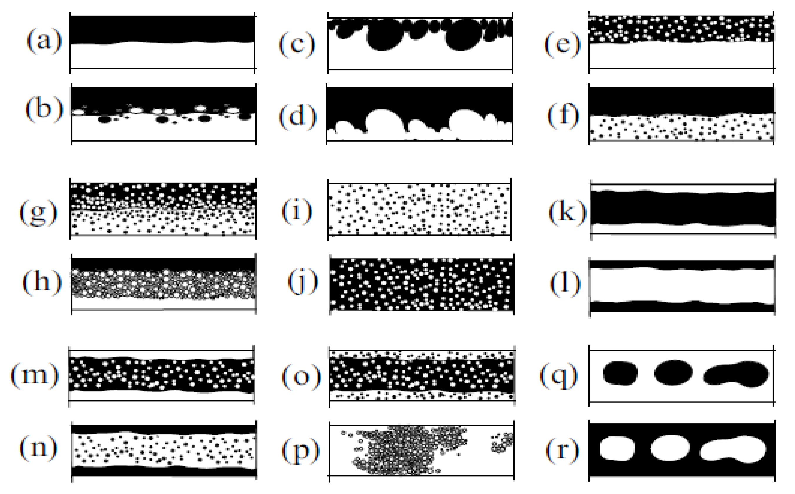
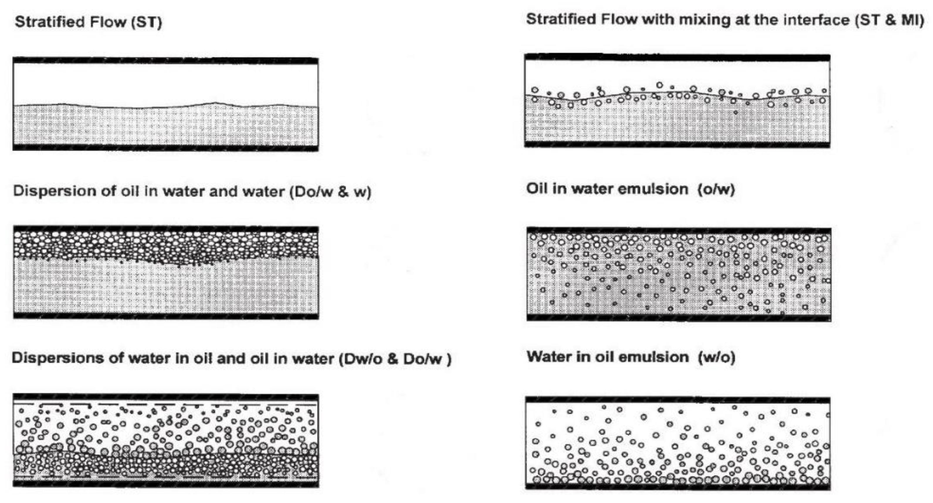
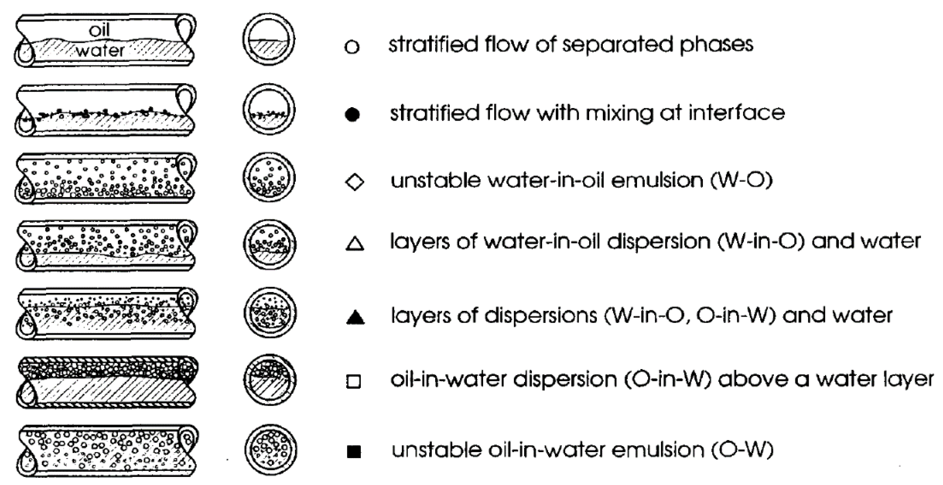
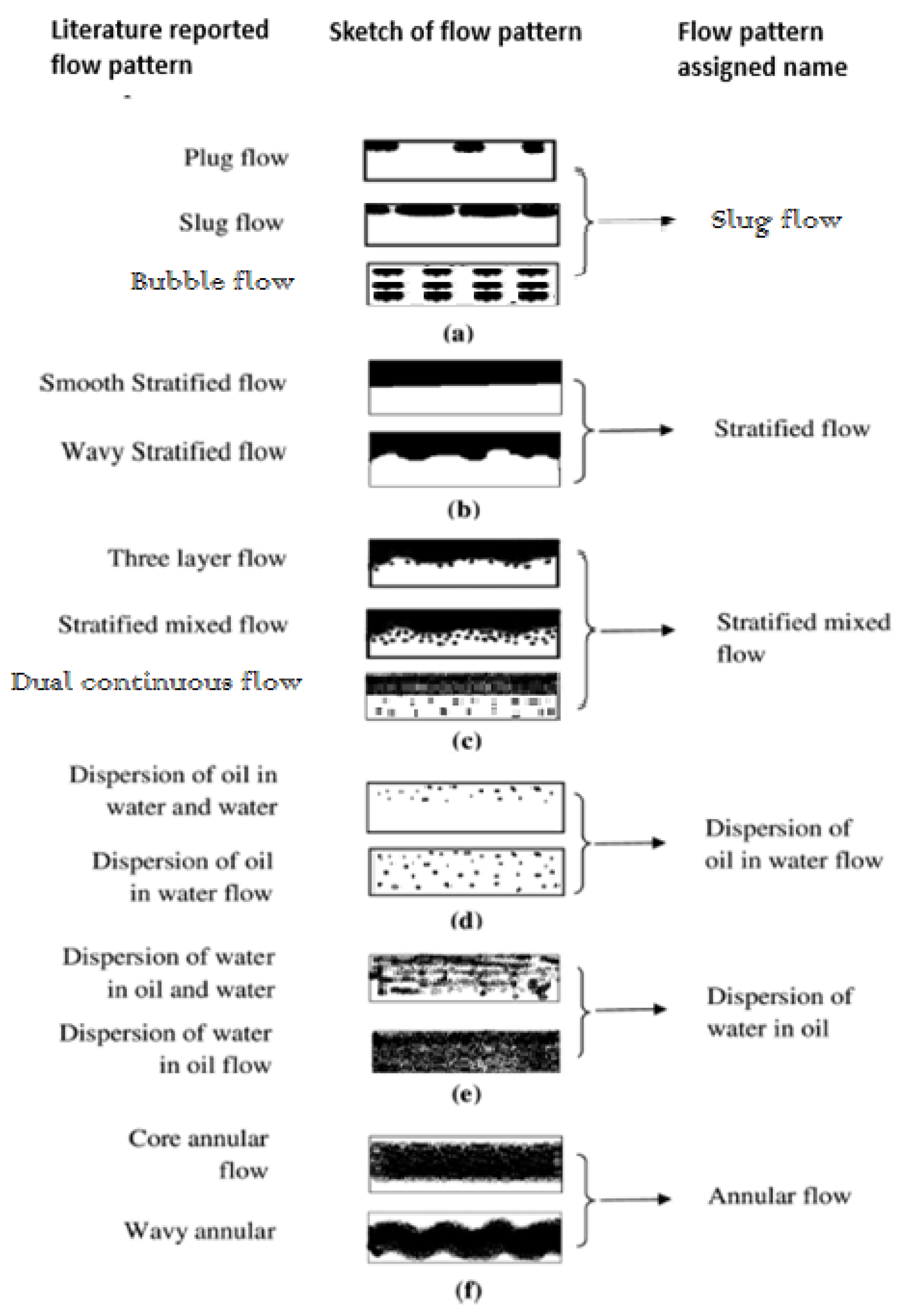
2.3. Harmonising the Major Flow Patterns in the Liquid-Liquid Horizontal Flow Literature

Due to different names and terminologies used by various investigators to describe each of the flow patterns, it is difficult to combine or compare flow patterns. For simplicity and standardisation, flow patterns from different investigators that share common features are grouped and classified into slug flow, stratified flow, stratified mixed flow, dispersed oil-in-water flow, dispersed water-in-oil flow, and annular flow as shown in Figure 5. The flow patterns by Trallero et al. [11] is one of the most adopted flow patterns among researchers, but it fails to report slug and annular flow patterns. Annular flow tends to occur easily when oil viscosity is high, with a critical value of 35 mPa s [15,54], or if the oil density is close to the water density [7,15,42], or if the pipe diameter is small [15,34,64]. Unlike the gas-liquid flow patterns, which are sensitive to pipe diameters, the liquid-liquid flow patterns are more susceptible to the properties of the liquids such as interfacial tension, density, and viscosity [15]. Usually, for small diameter pipes (10 mm and smaller), different flow patterns were observed, such as the plug, slug, churn, and rivulet [64].

3. Dimensionless Parameter Definition

There are three main approaches to defining the dimensionless groups characterising a liquid-liquid flow system [65]. These include dimensionless analysis, dynamic and kinematic ratio analysis, and basic equation analysis [65]. For dimensionless analysis, the Buckingham Π theorem can be applied to the independent system variables and fundamental dimensions of the oil-water flow to determine the governing dimensionless groups [5]. For a fully developed, steady-state, isothermal oil-water flow in a horizontal pipeline, there are eleven relevant independent variables [5]. These include superficial oil and water velocities (v_so) and (v_sw), oil and water densities (ρ_o), and (ρ_w), pipe diameter (d), oil and water viscosities (µ_o) and (µ_w), interfacial tension (σ), pipe roughness (ε), the acceleration due to gravity (g), and wettability (α) (assumption: for horizontal orientation neglect inclination angle (ϴ)). While the three fundamental dimensions are mass (M), length (L) and time (T). Based on Buckingham Π theorem, the number of system variables minus the number of fundamental variables is equal to the number of dimensionless groups [65]. Hence, eight dimensionless groups are expected from oil-water flow system, which Ibarra et al. [5] gave as (i) wettability, (ii) relative roughness, (iii) density ratio, (iv) viscosity ratio, (v) water fraction, (vi) mixture Reynold number, (vii) Eötvös number and (viii) mixture Froude number. However, Langhaar [66] and Shoham [65] stated that the formed dimensionless groups could be recombined to produce other groups not formed from the dimensionless analysis; in other words, by recombining the results of the dimensional analysis, one could generate an infinite/innumerable number of groups.

Plotting the superficial water velocity (v_sw = Q_w/A) versus the superficial oil velocity (v_so = Q_o/A) is a common way of constructing flow pattern maps, where A is the cross-sectional area of the pipe and Q_o and Q_w are the volumetric flow rates of oil and water, respectively [10]. A flow pattern map for a two-phase flow system depends on the geometrical variables (pipe diameter and inclination angle), the fluid physical properties (densities, viscosities and surface tension) and operational variables (phase flow rates) [19,25]. These types of flow pattern maps are dimensional in that they are usually valid only for the particular pipe sizes and fluids employed to construct the flow maps [4]. Construction of flow pattern maps based on some relevant dimensionless groups would enable the possibility to compare and combine different experimental data and to develop more generalised flow pattern maps, which would cover a wide range of flow systems [5].

Some dimensionless groups governing the liquid-liquid flow are the ratio of some forces acting on the flow system. The following forces (inertia, viscous, gravity (buoyancy) and interfacial tension (capillary)) influence the liquid-liquid flow in horizontal pipelines [5]. Therefore, the effect of liquid properties (density, viscosity, and interfacial tension), pipe diameter and velocity are all included in the dimensionless parameters [5]. The ratio of the gravity force to the surface or interfacial tension force is expressed by the Eötvös number (Eo), presented in Equation (1). The Eötvös number (Eo) could predict the force that would be dominant in a liquid-liquid flow horizontal pipeline, based on the fluids properties and the internal pipe diameter.

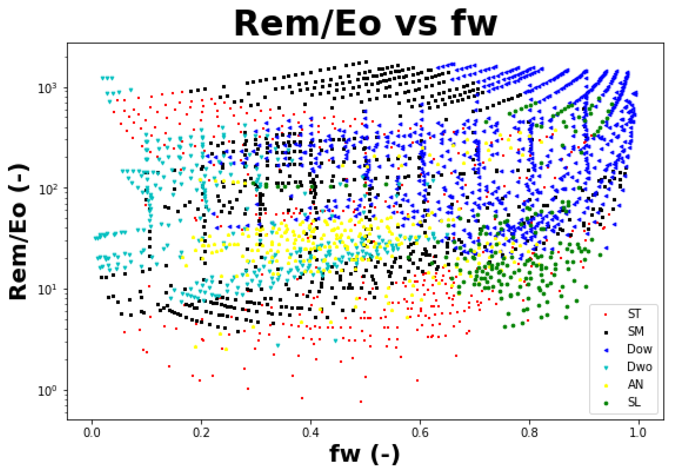
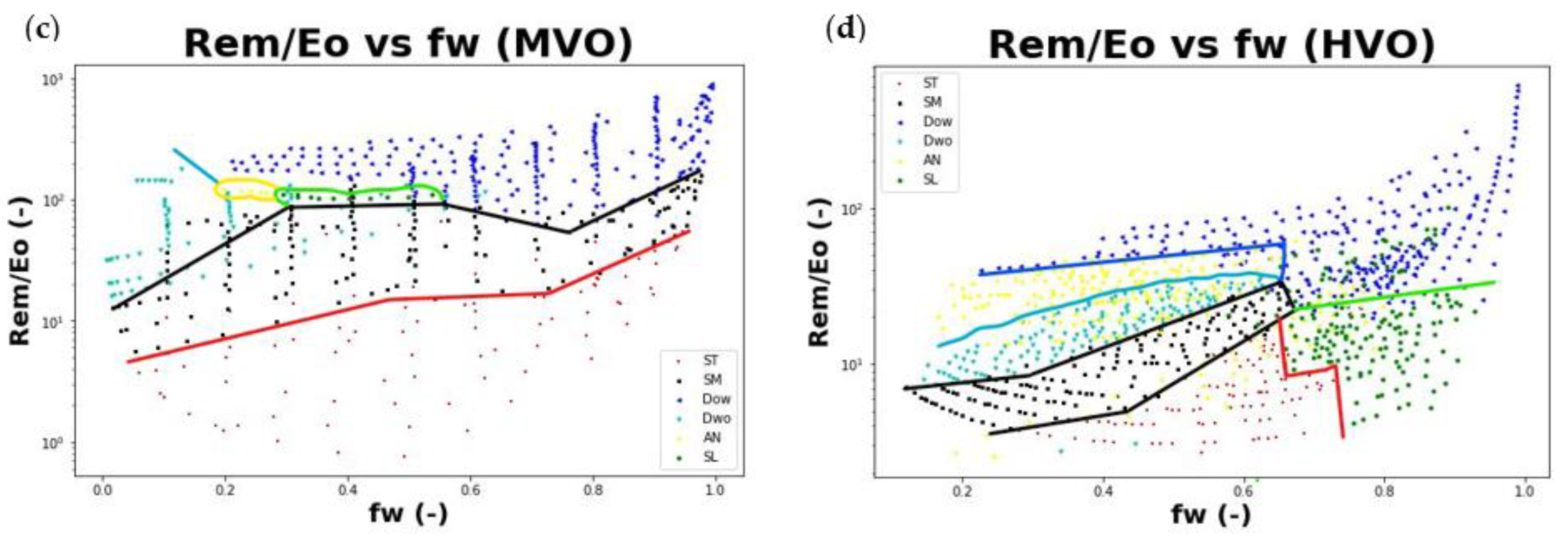
3.1. Mixture Reynolds Number to Eötvös number (Re_m/Eo)

The Reynolds number (Re) is the ratio of the inertia force to viscous force in a flow system, while the mixture Reynolds number (Re_m) can be expressed as

$${\mathrm{Re}}_{\mathrm{m}}=\frac{{\mathsf{\rho }}_{\mathrm{m}}{\mathrm{v}}_{\mathrm{m}}\mathrm{d}}{{\mathsf{\mu }}_{\mathrm{m}}}$$

(3)

To calculate Re_m from the homogeneous flow model, one must treat a liquid-liquid flow as a pseudo-single phase liquid with average liquid properties and average velocity [65]. Hence, in determining the thermal and fluid-dynamics behaviours of the fluid, no interface exchange is considered and only one mixture velocity, one mixture pressure and one mixture temperature are used [67,68]. The mixture velocity (v_m), mixture density (ρ_m), and mixture viscosity (µ_m) can be expressed in terms of volume fraction or mass fraction assuming no-slip conditions [5,65,69].

$${\mathrm{v}}_{\mathrm{m}}=\frac{{\mathrm{Q}}_{\mathrm{w}}+{\mathrm{Q}}_{\mathrm{o}}}{\mathrm{A}}={\mathrm{v}}_{\mathrm{sw}}+{\mathrm{v}}_{\mathrm{so}},$$

(4)

$${\mathsf{\rho }}_{\mathrm{m}}={\mathsf{\rho }}_{\mathrm{w}}{\mathrm{f}}_{\mathrm{w}}+{\mathsf{\rho }}_{\mathrm{o}}\left(1-{\mathrm{f}}_{\mathrm{w}}\right),$$

(5)

$${\mathrm{\mu }}_{\mathrm{m}}={\mathrm{\mu }}_{\mathrm{w}}{\mathrm{f}}_{\mathrm{w}}+{\mathrm{\mu }}_{\mathrm{o}}\left(1-{\mathrm{f}}_{\mathrm{w}}\right)$$

(6)

where f_w is the water fraction, calculated as

$${\mathrm{f}}_{\mathrm{w}}=\frac{{\mathrm{Q}}_{\mathrm{w}}}{{\mathrm{Q}}_{\mathrm{w}+}{\mathrm{Q}}_{\mathrm{o}}}=\frac{{\mathrm{v}}_{\mathrm{sw}}}{{\mathrm{v}}_{\mathrm{sw}}+{\mathrm{v}}_{\mathrm{sw}}},$$

(7)

Then, the ratio can be expressed as

$$\frac{{\mathrm{Re}}_{\mathrm{m}}}{\mathrm{Eo}}=\frac{{\mathsf{\rho }}_{\mathrm{m}}{\mathrm{v}}_{\mathrm{m}}}{{\mathsf{\mu }}_{\mathrm{m}}}\frac{\mathsf{\sigma }}{\Delta \mathsf{\rho }\mathrm{g}\mathrm{d}}$$

(8)

The ratio of mixture Reynolds number to Eötvös number Re_m/Eo as a function of water fraction (f_w) has been applied by Ibarra et al. [5] to create a dimensionless flow pattern transitions map.

3.2. Weber Number to Eötvös Number (We/Eo)

The Weber number is the ratio of inertia force to the interfacial tension force, while the ratio of the difference in the two-phase gravity forces to interfacial tension force is called the Eötvös number. Therefore, the We/Eo can be expressed as the ratio of inertia force to the difference in the two-phase gravity forces.

$$\frac{\mathrm{We}}{\mathrm{Eo}}=\frac{{\mathsf{\rho }}_{\mathrm{m}}{\mathrm{v}}_{\mathrm{m}}^2}{\Delta \mathsf{\rho }\mathrm{g}\mathrm{d}}$$

(9)

A high We/Eo depicts the dominance of inertia force over buoyancy, where the flow will be turbulent, and there will be instabilities at the interface between the two liquids. The dispersed flows are the most likely flow patterns in this region. At low We/Eo, the gravity forces dominate, hence the gravitational effect will make the dense liquid to flow at the bottom of the pipe while the light liquid flows at the top. The most likely flow pattern is stratified flow.

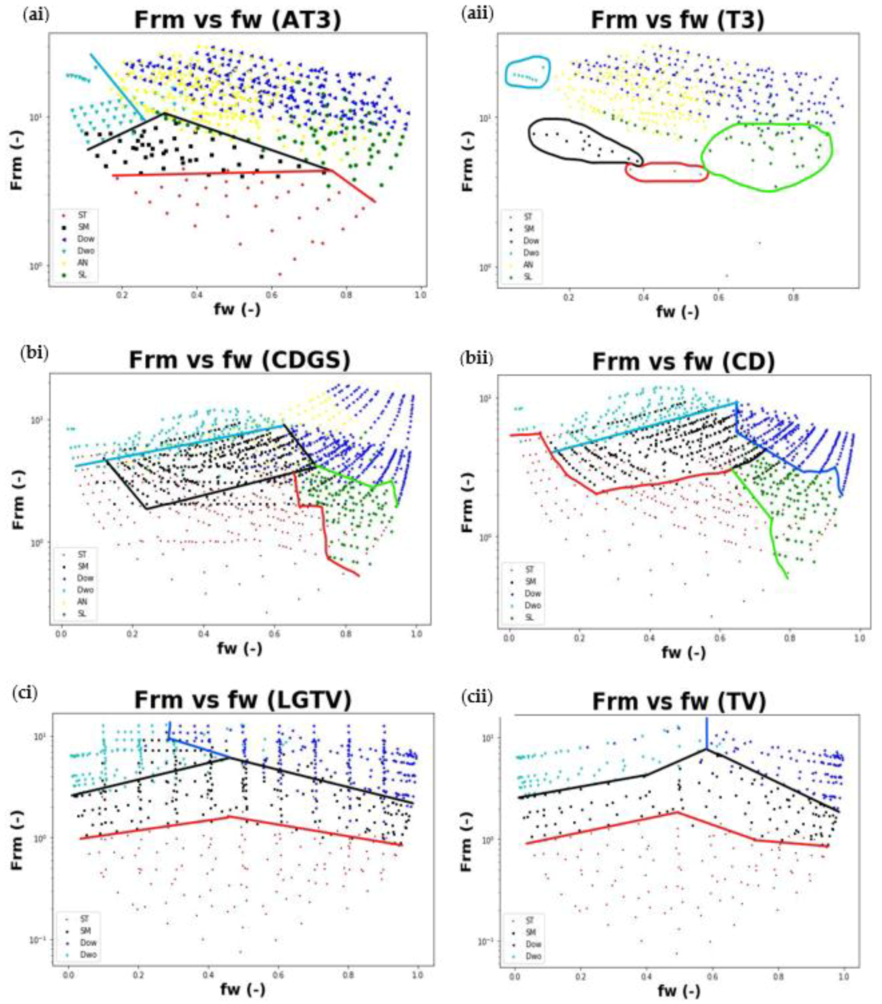
3.3. Mixture Froude Number (Fr_m), Oil Froude Number (Fr_o) and Water Froude Number (Fr_w)

The mixture Froude number (Fr_m) is the ratio of inertia force to the gravity force based on the average properties of the two immiscible fluids (oil and water) as explained by the mixture Reynolds number to Eötvös number (Re_m/Eo).

$${\mathrm{Fr}}_{\mathrm{m}}^2=\frac{{\mathrm{v}}_{\mathrm{m}}^2}{\mathrm{gd}}\frac{{\mathsf{\rho }}_{\mathrm{m}}}{\left({\mathsf{\rho }}_{\mathrm{w}}-{\mathsf{\rho }}_{\mathrm{o}}\right)}$$

(10)

$${\mathrm{Fr}}_{\mathrm{O}}^2=\frac{{\mathrm{v}}_{\mathrm{O}}^2}{\mathrm{gd}}\frac{{\mathsf{\rho }}_{\mathrm{O}}}{\left({\mathsf{\rho }}_{\mathrm{w}}-{\mathsf{\rho }}_{\mathrm{o}}\right)}$$

(11)

$${\mathrm{Fr}}_{\mathrm{W}}^2=\frac{{\mathrm{v}}_{\mathrm{W}}^2}{\mathrm{gd}}\frac{{\mathsf{\rho }}_{\mathrm{W}}}{\left({\mathsf{\rho }}_{\mathrm{w}}-{\mathsf{\rho }}_{\mathrm{o}}\right)}$$

(12)

By definition, both We/Eo and Fr_m are ratios of inertia force to the gravity force so that one can determine the relationship between them.

Divide We/Eo by Fr_m

$$\frac{\frac{\mathrm{We}}{\mathrm{Eo}}}{{\mathrm{Fr}}_{\mathrm{m}}^2}=\frac{\frac{{\mathsf{\rho }}_{\mathrm{m}}{\mathrm{v}}_{\mathrm{m}}^2}{\Delta \mathsf{\rho }\mathrm{g}\mathrm{d}}}{\frac{{\mathrm{v}}_{\mathrm{m}}^2}{\mathrm{gd}}\frac{{\mathsf{\rho }}_{\mathrm{m}}}{\left({\mathsf{\rho }}_{\mathrm{w}}-{\mathsf{\rho }}_{\mathrm{o}}\right)}}=1$$

(13)

Hence,

$${\mathrm{Fr}}_{\mathrm{m}} ={\left(\frac{\mathrm{We}}{\mathrm{Eo}}\right)}^{1/2}$$

(14)

The turbulence of We/Eo will be the square of the turbulence of Fr_m when the inertia force is dominant. Dispersed flow patterns are more likely in this region. Where gravity force is dominant, the gravitational effect will be high, which will cause the stratification of the oil and water flow, and the value of Fr_m will be a square root of the We/Eo value. Both Fr_m and We/Eo give the same information but at different magnitudes.

3.4. Gravity Force to Viscous Force (G/V)

The ratio of gravity and viscous forces for the oil-water flows is represented as G/V [61]. At high G/V in oil-water flows, the gravity force dominates, while the viscous force is comparatively low (i.e., low oil viscosity, since water viscosity is constant). For this case, the fluid will break up easily at high kinetic energy, and the most likely flow structures are stratified flow and fine dispersions of one of the liquids in the continuum of the other [61]. At low G/V in oil-water flow, the stratified flow is less likely to form because the gravitational force effect is comparatively small. The probable flow configurations are oil core flowing inside annular water: continuously to generate annular (core annular flow) or discontinuously to produce intermittent flows (slug, plug) in which shear stress is minimal [61]. With high turbulence kinetic energy flow, the higher viscous (oil) phase is too viscous to be broken by the kinetic energy into fine drops but lumps of various sizes and shapes. For a liquid-liquid flow with medium G/V, both the gravity and viscous forces influence this region, and all the flow patterns can occur within the region.

4. Results

4.1. Data Sources

Data gathering and analysis are presented. All the datasets used in developing some flow maps were obtained from liquid-liquid experimental works published in scholarly journals. The density of oil experimented in all the cases is less than water density, and all the considered experimental works were performed in the horizontal orientation. Brief details of each of the experimental works are presented in

Table 4. Sources of the gathered datasets.

Trallero et al. [11]		Soleimani [52]
Tap water density (kg/m3)	997 *	Tap water density (kg/m3)	998
White oil density (kg/m3)	884	Exxsol 80 density (kg/m3)	801
Tap water viscosity (Pa s)	0.00097	Tap water viscosity (Pa s)	0.001
White oil viscosity (Pa s)	0.0288	Exxsol 80 viscosity (Pa s)	0.0016
Interfacial tension (N/m)	0.036	Interfacial tension (N/m)	0.017 @ 22 °C
Diameter (m)	0.0501	Diameter (m)	0.0243
Temperature (°C)	25.5	Temperature (°C)	25
Al-Wahaibi et al. [22]		Vielma et al. [57]
Water density (kg/m3)	998	Tap water density (kg/m3)	998
Mineral oil density (kg/m3)	875	Mineral oil density (kg/m3)	860 **
Water viscosity (Pa s)	0.001	Tap water viscosity (Pa s)	0.001
Mineral oil viscosity (Pa s)	0.012	Mineral oil viscosity (Pa s)	0.0188 **
Interfacial tension (N/m)	0.0201	Interfacial tension (N/m)	0.0285 **
Diameter (m)	0.019	Diameter (m)	0.0508
Temperature (°C)	N/A	Temperature (°C)	25.5
Dasari et al. [58]		Guzhov et al. [38]
Water density (kg/m3)	997	Tap water density (kg/m3)	998
Lube oil density (kg/m3)	889	Mineral oil density (kg/m3)	896
Water viscosity (Pa s)	0.001	Tap water viscosity (Pa s)	0.001
Lube oil viscosity (Pa s)	0.107	Mineral oil viscosity (Pa s)	0.0218
Interfacial tension (N/m)	0.024	Interfacial tension (N/m)	0.0448
Diameter (m)	0.025	Diameter (m)	0.0394
Temperature (°C)	25	Temperature (°C)	21
Grassi et al. [41]		Tan et al. [3] 20#
Water density (kg/m3)	997	Tap water density (kg/m3)	998
Oil density (kg/m3)	886	Mineral oil density (kg/m3)	888
Water viscosity (Pa s)	0.0013	Tap water viscosity (Pa s)	0.001
Oil viscosity (Pa s)	0.653	Mineral oil viscosity (Pa s)	0.02
Interfacial tension (N/m)	0.05	Interfacial tension (N/m)	0.01897
Diameter (m)	0.021	Diameter (m)	0.0145
Temperature (°C)	25	Temperature (°C)	25
Chakrabarti et al. [56]		Tan et al. [3] 200#
Water density (kg/m3)	997	Tap water density (kg/m3)	998
Kerosine (kg/m3)	787	Mineral oil density (kg/m3)	869
Water viscosity (Pa s)	0.00084	Tap water viscosity (Pa s)	0.001
Kerosine (Pa s)	0.0012	Mineral oil viscosity (Pa s)	0.237
Interfacial tension (N/m)	0.045	Interfacial tension (N/m)	0.04583
Diameter (m)	0.0254	Diameter (m)	0.0145
Temperature (°C)	25	Temperature (°C)	25
Lovick and Angeli [55]		Tan et al. [3] 400#
Tap water density (kg/m3)	998	Tap water density (kg/m3)	998
Exxsol140 density (kg/m3)	828	Mineral oil density (kg/m3)	896
Tap water viscosity (Pa s)	0.001	Tap water viscosity (Pa s)	0.001
Exxsol140 viscosity (Pa s)	0.006	Mineral oil viscosity (Pa s)	0.456
Interfacial tension (N/m)	0.0396	Interfacial tension (N/m)	0.05149
Diameter (m)	0.038	Diameter (m)	0.0145
Temperature (°C)	25	Temperature (°C)	25

Note: for data with ⁽*⁾, the authors recorded 1037 kg/m³ for tap water at ≈25.5 °C. For data with ⁽**⁾, the authors compared these values with Trallero et al. [11] data; hence those values are considered to be at the same temperature with Trallero et al. [11] data.

.

Based on similar operating conditions for the considered experimental studies, water properties are quite similar, while oil density and oil viscosity range between 787–896 kg/m³ and 0.006–0.653 Pa s, respectively. The pipe diameter ranges between 0.0145–0.0508 m, while the interfacial tension ranges between 0.017–0.05149 N/m. Each source contributed datapoints to the datasets as follows: Trallero et al. [11] = 251, Soleimani [52] = 166, Al-Wahaibi et al. [22] = 196, Vielma et al. [57] = 153, Dasari et al. [58] = 538, Guzhov et al. [38] = 176, Grassi et al. [41] = 137, Tan et al. [3] 20# = 112, Chakrabarti et al. [56] = 506, Tan et al. [3] 200# = 224, Lovick and Angeli [55] = 114, and Tan et al. [3] 400# = 123.

4.2. Flow Pattern Maps Construction

Figure 6 presents a flow pattern map of the ratio of mixture Reynold number to Eötvös number (Re_m/Eo) versus water fraction (f_w), a representation of one of various combinations of dimensionless groups under consideration. The data were further classified based on oil viscosity and diameter to see if the data from a particular flow pattern would form a better cluster on the flow map. The results are discussed below.

4.2.1. Flow Pattern Maps Based on Oil Viscosity

Abubakar et al. [45] and Tan et al. [3] classified oil viscosity into <10 mPa s, 20–100 mPa s and >100 mPa s as low-viscous oil (LVO), medium-viscous oil (MVO) and heavy-viscous oil (HVO), respectively. Figure 7 presents flow maps of the ratio of mixture Reynold number to Eötvös number (Re_m/Eo) versus water fraction (f_w) after regrouping of data by oil viscosity.

The oil viscosity between 10–20 mPa s was missing in the classification, so another class of <20 mPa s was considered as only two of the selected experimental works have their oil viscosity in the range of 10–20 mPa s. The same analysis was performed using the other combination of dimensionless groups, and the results are presented in

Table 5. A summary of constructed flow pattern maps using dimensionless parameters.

	ST	SM	Do/w	Dw/o	SL	AN
Rem/Eo versus fw	N	N	N	N	N	N
Rem/Eo versus fw (LVO <10)	N	N	N	N	Y	N/A
Rem/Eo versus fw (LVO <20)	N	N	N	N	Y	N
Rem/Eo versus fw (MVO)	Y	Y	Y	Y	Y *	Y *
Rem/Eo versus fw (HVO)	Y	Y	Y	Y	Y	N
We/Eo versus fw	Y	Y	N	Y	Y	N
Frm versus fw	Y	Y	N	Y	Y	N
G/V versus fw	N	N	N	N	N	N
G/V versus fw (LVO <10)	Y	Y	Y	Y	Y	N/A
G/V versus fw (LVO <20)	N	N	N	Y	N	Y
G/V versus fw (MVO)	Y	N	N	N	Y	Y
G/V versus fw (HVO)	Y	Y	N	Y	N	Y
Frw versus Fro	N	N	N	N	N	N
Frw versus Fro (LVO <10)	Y	Y	Y	Y	Y	N/A
Frw versus Fro (LVO <20)	N	N	N	N	N	N
Frw versus Fro (MVO)	Y	Y	Y	Y	Y *	Y *
Frw versus Fro (HVO)	Y	Y	N	Y	N	N

Note: * means a few data points, Y means yes, flow pattern marked out, N means no, flow pattern not marked out, N/A means not applicable. Note: ST means stratified flow, SM means stratified mixed flow, Do/w means dispersed oil-in-water flow, Dw/o means dispersed water-in-oil, SL means slug flow and AN means annular flow.

.

4.2.2. Flow Pattern Maps Based on the Pipe Diameter

Cai et al. [15] showed that liquid-liquid flow patterns are less susceptible to pipe diameter, unlike gas-liquid flow patterns. However, it remains important to investigate the effect of pipe diameter on the flow patterns of liquid-liquid flows; this will be achieved by regrouping the data points based on the pipe diameter of the experimental set-up. Three classes of diameters considered, namely ≤20 mm, 21–30 mm and >30 mm, which are referred to as class 1, class 2 and class 3, respectively.

The combinations of dimensionless groups used for the analysis are (i) Re_m/Eo versus f_w, (ii) We/Eo versus f_w, (iii) Fr_m versus f_w, (iv) G/V versus f_w, (v) Fr_w versus Fr_o. Let Fr_m versus f_w be a representative combination of dimensionless groups to show the effect of pipe diameters on the liquid-liquid flow pattern in the horizontal pipeline, as presented in Figure 8. The experimental works in class 1 are those of Al-Wahaibi et al. [22] and Tan et al. [3] 20#, 200# & 400# with diameters of 19 and 14.5 mm, respectively. The experimental works in class 2 are taken from Chakrabarti et al. [56], Dasari et al. [58], Grassi et al. [41], and Soleimani [52] with diameters of 25.4, 25, 21, and 24.3 mm, respectively. The experimental works in class 3 are those of Guzhov et al. [38], Lovick and Angeli [55], Trallero et al. [11], and Vielma et al. [57] with diameters of 39.4, 38, 50.1, and 50.8 mm, respectively.

5. Discussion

5.1. Data Analysis

The use of dimensionless groups is to normalise the data points of a particular flow pattern so that the data points can form a distinct region on a flow map. The gathered datasets are placed in six classes of flow patterns, which are stratified (ST), stratified mixed (SM), dispersed oil in water (Do/w), dispersed water in oil (Dw/o), annular (AN) and slug (SL) flows. There are several combinations of dimensionless groups that can be used for constructing a flow map and those considered in this work are: (i) the ratio of mixture Reynold number to Eötvös number (Re_m/Eo) versus water fraction (f_w), (ii) the ratio of Weber number to Eötvös number (We/Eo) versus water fraction (f_w), (iii) the mixture Froude number (Fr_m) versus water fraction (f_w), (iv) the ratio of gravity force to viscous force G/V versus water fraction (f_w), (v) the water Froude number (Fr_w) versus the oil Froude number (Fr_o).

The following combinations of dimensionless groups (Re_m/Eo versus f_w, G/V versus f_w, and Fr_w versus Fr_o) show that all flow patterns form more than one trend on the flow pattern map. Hence, there is no distinct region on the flow pattern map that can be designated for a particular flow pattern. Figure 6 gives a representation of these combinations of dimensionless groups. The data were further classified based on oil viscosity and diameter to see if the data from a particular flow pattern would form a better cluster on the flow map. The results are discussed below.

5.1.1. Data Analysis Based on Oil Viscosity

After regrouping the gathered data by oil viscosity, a better trend of the flow patterns was formed on the flow map in Figure 7 as compared to Figure 6, but not all the flow patterns could be delineated on the flow map. The flow patterns were better marked out when the data points were classified based on their oil viscosity in all cases, as presented in Table 5. However, all the flow patterns cannot be marked out on a flow map using any of the considered dimensionless group combinations, even where the oil viscosity is one of the variables in the formation of the combined dimensionless groups i.e., (i) Re_m/Eo versus f_w, (ii) G/V versus f_w, the flow patterns were still not completely normalised. In low-viscous oil (LVO) <20 mPa s category, Fr_w versus Fr_o normalised no flow pattern, Re_m/Eo versus f_w delineated only SL flow pattern, and G/V versus f_w normalised Dw/o and AN flow patterns. In low-viscous oil (LVO) <10 mPa s category, Fr_w versus Fr_o and G/V versus f_w normalised all the flow patterns available for the analysis, while Re_m/Eo versus f_w delineated only SL flow pattern. Hence, (LVO) <20 mPa s group may be too broad for the analysis.

5.1.2. Data Analysis Based on the Pipe Diameter

Figure 8ai contains experimental works with diameters 14.5 and 19 mm, while Figure 8aii contains experimental works with a diameter of 14.5 mm. The Fr_m versus f_w was expected to normalise the flow patterns, particularly as the diameter range was narrowed. However, the following flow patterns Dow, AN and SL, and Dow and AN could not be delineated in Figure 8ai and Figure 8aii, respectively.

Likewise, to check the effect of a slight change in diameter, the experimental works with diameters of 21, 24.3, 25 and 25.4 mm were plotted Figure 8bi, whilst the data associated with slightly bigger pipe diameters of 25.4 and 25 mm are shown in Figure 8bii. With a wider diameter range (Figure 8bi), the dimensionless groups do not normalise all the flow patterns, but with a slight change in diameter (Figure 8bii) all the flow patterns were normalised and delineated.

Figure 8ci has the experimental works with diameters of 39.4, 38, 50.1 and 50.8 mm, but Figure 8cii has a narrower diameter range of 50.1 and 50.8 mm. In both cases, the Fr_m versus f_w normalised and delineated the flow patterns.

6. Conclusions

A literature review on experimental studies and development of flow pattern maps of liquid-liquid flow in horizontal pipes were conducted. Relevant datasets were obtained from twelve experimental studies published in scholarly journals. The following combinations of dimensionless groups ((i) the ratio of mixture Reynold number to Eötvös number (Re_m/Eo) versus water fraction (f_w), (ii) the ratio of Weber number to Eötvös number (We/Eo) versus water fraction (f_w), (iii) the mixture Froude number (Fr_m) versus water fraction (f_w), (iv) the ratio of gravity force to viscous force (G/V) versus water fraction (f_w), (v) the water Froude number (Fr_w) versus the oil Froude number (Fr_o)) were used to obtain more generalised flow pattern maps.

• Based on the analysis done in this project, it can be concluded that each flow pattern formed more than one trend on the flow map when data from the twelve sources were brought together, hence no particular region can be designated to a particular flow pattern in such a flow map. In exception of the combinations, (i) We/Eo versus f_w and (ii) Fr_m versus f_w, where ST, SM, SL and Dw/o were marked out.
• However, the flow patterns formed clearer trends on the flow map when the data points were regrouped, based on the oil-phase viscosity and pipe diameter used in the experimental studies.
• For regrouping based on oil viscosity, combinations of the ratio of mixture Reynold number to Eötvös number (Re_m/Eo) versus water fraction (f_w), and water Froude number (Fr_w) versus oil Froude number (Fr_o) dimensionless groups marked out regions for all the considered flow patterns under the medium-viscous oil (MVO) category, though slug and annular flow patterns had only a few data points as compared to the other flow patterns.
• Under low-viscous oil (LVO) <10 group, there is no occurrence of annular flow, and hence the combination of these dimensionless groups G/V versus f_w, and Fr_w versus Fr_o were able to normalise all the data points so that each flow pattern formed on a distinct region on the flow map.
• Under heavy-viscous oil (HVO) group, the ratio of mixture Reynold number to Eötvös number (Re_m/Eo) versus water fraction (f_w) normalised all the data points except for the annular flow pattern. The ratio of gravity force to viscous force (G/V) versus water fraction (f_w) normalised all the data points except for dispersed oil in water and slug flow patterns, while the and water Froude number (Fr_w) versus the oil Froude number (Fr_o) could not normalise dispersed oil in water, slug and annular flow patterns.
• For the regrouping based on pipe diameters, as the range of considered pipe diameters narrows, the cluster of data points for each flow pattern forms a more distinct region on the flow map.

References

1. Angeli, P.; Hewitt, G.F. Pressure Gradient in Horizontal Liquid-Liquid Flows. Int. J. Multiph. Flow 1999, 24, 1183–1203. [Google Scholar] [CrossRef]
2. Brauner, N. Liquid-Liquid Two-Phase Flow Systems. In Modelling and Control of Two-Phase Phenomena; Bertola, V., Ed.; Springer: Vienna, Austria, 2003; pp. 221–279. [Google Scholar] [CrossRef]
3. Tan, J.; Jing, J.; Hu, H.; You, X. Experimental Study of the Factors Affecting the Flow Pattern Transition in Horizontal Oil–Water Flow. Exp. Therm. Fluid Sci. 2018, 98, 534–545. [Google Scholar] [CrossRef]
4. Brennen, C.E. Fundamentals of Multiphase Flow; Cambridge University Press: Cambridge, UK, 2005. [Google Scholar]
5. Ibarra, R.; Zadrazil, I.; Markides, C.N.; Matar, O.K. Towards a Universal Dimensionless Map of Flow Regime. In Proceedings of the 11th International Conference on Heat Transfer, Fluid Mechanics and Thermodynamics, Skukuza, South Africa, 20–23 July 2015. [Google Scholar]
6. Russell, T.W.F.; Hodgson, G.W.; Govier, G.W. Horizontal Pipeline Flow of Mixtures of Oil and Water. Can. J. Chem. Eng. 1959, 37, 9–17. [Google Scholar] [CrossRef]
7. Charles, M.E.; Govier, G.W.; Hodgson, G.W. The Horizontal Pipeline Flow of Equal Density Oil-water Mixtures. Can. J. Chem. Eng. 1961, 39, 27–36. [Google Scholar] [CrossRef]
8. Charles, M.E.; Lilleleht, L.V. Correlation of Pressure Gradients for the Stratified Laminar-turbulent Pipeline Flow of Two Immiscible Liquids. Can. J. Chem. Eng. 1966, 44, 47–49. [Google Scholar] [CrossRef]
9. Valle, A. Multiphase Pipeline Flows in Hydrocarbon Recovery. Multiph. Sci. Technol. 1998, 10, 1–139. [Google Scholar] [CrossRef]
10. Ahmed, S.A.; John, B. Liquid-Liquid Horizontal Pipe Flow—A Review. J. Pet. Sci. Eng. 2018, 168, 426–447. [Google Scholar] [CrossRef]
11. Trallero, J.L.; Sarica, C.; Brill, J.P. A Study of Oil/Water Flow Patterns in Horizontal Pipes. In SPE Annual Technical Conference and Exhibition; Society of Petroleum Engineers: Dallas, TX, USA, 1997; pp. 165–172. [Google Scholar] [CrossRef]
12. Al-Sarkhi, A.; Pereyra, E.; Mantilla, I.; Avila, C. Dimensionless Oil-Water Stratified to Non-Stratified Flow Pattern Transition. J. Pet. Sci. Eng. 2017, 151, 284–291. [Google Scholar] [CrossRef]
13. Paolinelli, L.D.; Rashedi, A.; Yao, J.; Singer, M. Study of Water Wetting and Water Layer Thickness in Oil-Water Flow in Horizontal Pipes with Different Wettability. Chem. Eng. Sci. 2018, 183, 200–214. [Google Scholar] [CrossRef]
14. Efird, K.D.; Jasinski, R.J. Effect of the Crude Oil on Corrosion of Steel in Crude Oil/Brine Production. Corrosion 1989, 45, 165–171. [Google Scholar] [CrossRef]
15. Cai, J.; Li, C.; Tang, X.; Ayello, F.; Richter, S.; Nesic, S. Experimental Study of Water Wetting in Oil-Water Two Phase Flow-Horizontal Flow of Model Oil. Chem. Eng. Sci. 2012, 73, 334–344. [Google Scholar] [CrossRef]
16. Shi, J.; Lao, L.; Yeung, H. Water-Lubricated Transport of High-Viscosity Oil in Horizontal Pipes: The Water Holdup and Pressure Gradient. Int. J. Multiph. Flow 2017, 96, 70–85. [Google Scholar] [CrossRef] [Green Version]
17. Arirachakaran, S.; Oglesby, K.D.; Malinowsky, M.S.; Shoham, O.; Brill, J.P. An Analysis of Oil/Water Flow Phenomena in Horizontal Pipes. In SPE Production & Facilities; Society of Petroleum Engineers: Dallas, TX, USA, 1989. [Google Scholar]
18. Mukhaimer, A.; Al-sarkhi, A.; El Nakla, M.; Ahmed, W.H.; Al-hadhrami, L. Effect of Water Salinity on Flow Pattern and Pressure Drop in Oil-Water Flow. J. Pet. Sci. Eng. 2015, 128, 145–149. [Google Scholar] [CrossRef]
19. Piroozian, A.; Hemmati, M.; Ismail, I.; Manan, M.A.; Rashidi, M.M.; Mohsin, R. An Experimental Study of Flow Patterns Pertinent to Waxy Crude Oil-Water Two-Phase Flows. Chem. Eng. Sci. 2017, 164, 313–332. [Google Scholar] [CrossRef]
20. Oglesby, K.D. An Experimental Study on the Effect of Oil Viscosity, Mixture Velocity and Water Fraction on Horizontal Oil-Water Flow. Master’s Thesis, The University of Tulsa, Tulsa, OK, USA, 1979. [Google Scholar]
21. Nädler, M.; Mewes, D. Flow Induced Emulsification in the Flow of Two Immiscible Liquids in Horizontal Pipes. Int. J. Multiph. Flow 1997, 23, 55–68. [Google Scholar] [CrossRef]
22. Al-Wahaibi, T.; Al-Wahaibi, Y.; Al-Ajmi, A.; Al-Hajri, R.; Yusuf, N.; Olawale, A.S.; Mohammed, I.A. Experimental Investigation on Flow Patterns and Pressure Gradient through Two Pipe Diameters in Horizontal Oil-Water Flows. J. Pet. Sci. Eng. 2014, 122, 266–273. [Google Scholar] [CrossRef]
23. Almutairi, Z.; Al-Alweet, F.M.; Alghamdi, Y.A.; Almisned, O.A.; Alothman, O.Y. Investigating the Characteristics of Two-Phase Flow Using Electrical Capacitance Tomography (ECT) for Three Pipe Orientations. Processes 2020, 8, 51. [Google Scholar] [CrossRef] [Green Version]
24. Cheng, L.; Ribatski, G.; Thome, J.R. Two-Phase Flow Patterns and Flow-Pattern Maps: Fundamentals and Applications. Appl. Mech. Rev. 2008, 61, 0508021–05080228. [Google Scholar] [CrossRef]
25. Torres, C.F.; Mohan, R.S.; Gomez, L.E.; Shoham, O. Oil-Water Flow Pattern Transition Prediction in Horizontal Pipes. J. Energy Resour. Technol. 2016, 138, 1–11. [Google Scholar] [CrossRef]
26. Hanafizadeh, P.; Hojati, A.; Karimi, A. Experimental Investigation of Oil-Water Two Phase Flow Regime in an Inclined Pipe. J. Pet. Sci. Eng. 2015, 136, 12–22. [Google Scholar] [CrossRef]
27. Cheng, H.; Hills, J.H.; Azzorpardi, B.J. A Study of the Bubble-to-Slug Transition in Vertical Gas-Liquid Flow in Columns of Different Diameter. Int. J. Multiph. Flow 1998, 24, 431–452. [Google Scholar] [CrossRef]
28. Al-Wahaibi, T.; Yusuf, N.; Al-Wahaibi, Y.; Al-Ajmi, A. Experimental Study on the Transition between Stratified and Non-Stratified Horizontal Oil-Water Flow. Int. J. Multiph. Flow 2012, 38, 126–135. [Google Scholar] [CrossRef]
29. Yusuf, N.; Al-Wahaibi, Y.; Al-Wahaibi, T.; Al-Ajmi, A.; Olawale, A.S.; Mohammed, I.A. Effect of Oil Viscosity on the Flow Structure and Pressure Gradient in Horizontal Oil-Water Flow. Chem. Eng. Res. Des. 2012, 90, 1019–1030. [Google Scholar] [CrossRef]
30. Angeli, P.; Hewitt, G.F. Flow Structure in Horizontal Oil-Water Flow. Int. J. Multiph. Flow 2000, 26, 1117–1140. [Google Scholar] [CrossRef]
31. Huang, Z.; Lee, H.S.; Senra, M.; Scott Fogler, H. A Fundamental Model of Wax Deposition in Subsea Oil Pipelines. AIChE J. 2011, 57, 2955–2964. [Google Scholar] [CrossRef] [Green Version]
32. Tritton, D.J. Physical Fluid Dynamics; Springer: Dordrecht, The Netherlands, 1977. [Google Scholar] [CrossRef]
33. Hasson, D.; Mann, V.; Nir, A. Annular Flow of Two Immiscible Liquids I. Mechanisms. Can. J. Chem. Eng. 1970, 48, 514–520. [Google Scholar] [CrossRef]
34. Wegmann, A.; von Rohr, P.R. Two Phase Liquid-Liquid Flows in Pipes of Small Diameters. Int. J. Multiph. Flow 2006, 32, 1017–1028. [Google Scholar] [CrossRef]
35. Valle, A.; Utvik, O.H. Pressure Drop, Flow Pattern and Slip for Two-Phase Crude Oil/Water Flow: Experiments and Model Predictions. In International Symposium on Liquid-Liquid Two-Phase Flow and Transport Phenomena; Begellhouse: Danbury, CT, USA, 1997; pp. 1–12. [Google Scholar] [CrossRef]
36. Vedapuri, D.; Bessette, D.; Jepson, W.P. A Segregated Flow Model to Predict Water Layer Thickness in Oil-Water Flows in Horizontal and Slightly Inclined Pipelines. In Proceedings of the 8th International Conference Multiphase ’97, Cannes, France, 18–20 June 1997; BHR Group, Ed.; Mechanical Engineering Publications: London, UK, 1997; pp. 75–106. [Google Scholar]
37. Simmons, M.J.H.; Azzopardi, B.J. Drop Size Distributions in Dispersed Liquid-Liquid Pipe Flow. Int. J. Multiph. Flow 2001, 27, 843–859. [Google Scholar] [CrossRef]
38. Guzhov, A.I.; Grishin, A.D.; Medredev, V.F.; Medredeva, O.P. Emulsion Formation during the Flow of Two Immiscible Liquids. Neft. Choz. 1973, 8, 58–61. (In Russian) [Google Scholar]
39. Brauner, N.; Moalem Maron, D. Flow Pattern Transitions in Two-Phase Liquid-Liquid Flow in Horizontal Tubes. Int. J. Multiph. Flow 1992, 18, 123–140. [Google Scholar] [CrossRef]
40. Ismail, A.S.I.; Ismail, I.; Zoveidavianpoor, M.; Mohsin, R.; Piroozian, A.; Sariman, M.Z.; Misnan, M.S. Review of Oil-Water through Pipes. Flow Meas. Instrum. J. 2015, 45, 357–374. [Google Scholar] [CrossRef]
41. Grassi, B.; Strazza, D.; Poesio, P. Experimental Validation of Theoretical Models in Two-Phase High-Viscosity Ratio Liquid-Liquid Flows in Horizontal and Slightly Inclined Pipes. Int. J. Multiph. Flow 2008, 34, 950–965. [Google Scholar] [CrossRef]
42. Bannwart, A.C.; Rodriguez, O.M.H.; de Carvalho, C.H.M.; Wang, I.S.; Vara, R.M.O. Flow Patterns in Heavy Crude Oil-Water Flow. J. Energy Resour. Technol. 2004, 126, 184. [Google Scholar] [CrossRef]
43. Bannwart, A.C. Wavespeed and Volumetric Fraction in Core Annular Flow. Int. J. Multiph. Flow 1998, 24, 961–974. [Google Scholar] [CrossRef]
44. Bordalo, S.N.; Oliveira, R.C. Experimental Study of Oil/ Water Flow With Paraffin Precipitation in Subsea Pipelines. In SPE Annual Technical Conference and Exhibition; Society of Petroleum Engineers: Dallas, TX, USA, 2007; pp. 1–8. [Google Scholar] [CrossRef]
45. Abubakar, A.; Al-Wahaibi, Y.; Al-Wahaibi, T.; Al-Hashmi, A.; Al-Ajmi, A.; Eshrati, M. Effect of Low Interfacial Tension on Flow Patterns, Pressure Gradients and Holdups of Medium-Viscosity Oil/Water Flow in Horizontal Pipe. Exp. Therm. Fluid Sci. 2015, 68, 58–67. [Google Scholar] [CrossRef]
46. Al-wahaibi, T.; Angeli, P. Experimental Study on Interfacial Waves in Stratified Horizontal Oil-Water Flow. Int. J. Multiph. Flow 2011, 37, 930–940. [Google Scholar] [CrossRef]
47. Wang, W.; Gong, J. Flow Regimes and Transition Characters of the High Viscosity Oil-Water Two Phase Flow. In Proceedings of the CPS/SPE International Oil & Gas Conference and Exhibition, Beijing, China, 8–10 June 2010; pp. 1–8. [Google Scholar] [CrossRef]
48. Gafonova, O.V.; Yarranton, H.W. The Stabilization of Water-in-Hydrocarbon Emulsions by Asphaltenes and Resins. J. Colloid Interface Sci. 2001, 241, 469–478. [Google Scholar] [CrossRef]
49. Angeli, P. Liquid-Liquid Dispersed Flows in Horizontal Pipes. Ph.D. Thesis, Imperial College London, London, UK, 1996. [Google Scholar]
50. Trallero, J.L. Oil-Water Flow Patterns in Horizontal Pipes. Ph.D. Thesis, The University of Tulsa, Tulsa, OK, USA, 1995. [Google Scholar]
51. Kurban, A.P.A.; Angeli, P.A.; Mendestatsis, M.A.; Hewitt, G.F. Stratified and Dispersed Oil-Water Flows in Horizontal Pipes. In Proceedings of the Multiphase 95, 7th International Conference, Cannes, France, 7–9 June 1995; pp. 277–291. [Google Scholar]
52. Soleimani, A. Phase Distribution and Associated Phenomena in Oil-Water Flows in Horizontal Tubes. Ph.D. Thesis, University of London, London, UK, 1999. [Google Scholar]
53. Mu, H. Experimental Research on Oil–Water Horizontal Pipe Flow. Master’s Thesis, University of Petroleum, Beijing, China, 2001. [Google Scholar]
54. Xu, X.X. Study on Oil-Water Two-Phase Flow in Horizontal Pipelines. J. Pet. Sci. Eng. 2007, 59, 43–58. [Google Scholar] [CrossRef]
55. Lovick, J.; Angeli, P. Experimental Studies on the Dual Continuous Flow Pattern in Oil-Water Flows. Int. J. Multiph. Flow 2004, 30, 139–157. [Google Scholar] [CrossRef]
56. Chakrabarti, D.P.; Das, G.; Ray, S. Pressure Drop in Liquid-Liquid Two Phase Horizontal Flow: Experiment and Prediction. Chem. Eng. Technol. 2005, 28, 1003–1009. [Google Scholar] [CrossRef]
57. Vielma, M.; Atmaca, S.; Sarica, C.; Zhang, H.Q. Characterization of Oil/Water Flows in Horizontal Pipes. In SPE Annual Technical Conference and Exhibition; Society of Petroleum Engineers: Dallas, TX, USA, 2007. [Google Scholar] [CrossRef]
58. Dasari, A.; Desamala, A.B.; Dasmahapatra, A.K.; Mandal, T.K. Experimental Studies and Probabilistic Neural Network Prediction on Flow Pattern of Viscous Oil-Water Flow through a Circular Horizontal Pipe. Ind. Eng. Chem. Res. 2013, 52, 7975–7985. [Google Scholar] [CrossRef]
59. Voulgaropoulos, V.; Zhai, L.; Loannou, K.; Angeli, P. Evolution of Unstable Liquid-Liquid Dispersions in Horizontal Pipes. In Proceedings of the BHR Group-10th North American Conference on Multiphase Technology 2016, Banff, AB, Canada, 8–10 June 2016; pp. 305–318. [Google Scholar]
60. Hapanowicz, J. Phase Inversion in Liquid-Liquid Pipe Flow. Flow Meas. Instrum. 2010, 21, 284–291. [Google Scholar] [CrossRef]
61. Shi, J.; Yeung, H. Characterization of Liquid-Liquid Flows in Horizontal Pipes. AIChE J. 2017, 63, 1132–1143. [Google Scholar] [CrossRef]
62. Joseph, D.D.; Nguyen, K.; Beavers, G.S. Non-Uniqueness and Stability of the Configuration of Flow of Immiscible Fluids with Different Viscosities. J. Fluid Mech. 1984, 141, 319–345. [Google Scholar] [CrossRef]
63. Ibarra, R.; Markides, C.N.; Matar, O.K. A Review of Liquid-Liquid Flow Patterns in Horizontal and Slightly Inclined Pipes. Multiph. Sci. Technol. 2014, 26, 171–198. [Google Scholar] [CrossRef]
64. Mandal, T.K.; Chakrabarti, D.P.; Das, G. Oil Water Flow through Different Diameter Pipes: Similarities and Differences. Chem. Eng. Res. Des. 2007, 85, 1123–1128. [Google Scholar] [CrossRef]
65. Shoham, O. Mechanistic Modeling of Gas Liquid Two Phase Flow in Pipes; The Society of Petroleum Engineers (SPE): Tulsa, OK, USA, 2005. [Google Scholar]
66. Langhaar, H.L. Dimensional Analysis and Theory of Model; John Wiley & Sons, Inc.: New York, NY, USA, 1951. [Google Scholar]
67. Morales-Ruiz, S.; Rigola, J.; Rodriguez, I.; Oliva, A. Numerical Resolution of the Liquid-Vapour Two-Phase Flow by Means of the Two-Fluid Model and a Pressure Based Method. Int. J. Multiph. Flow 2012, 43, 118–130. [Google Scholar] [CrossRef]
68. Levy, S. Two-Phase Flow in Complex Systems; John Wiley & Sons: Hoboken, NJ, USA, 1999. [Google Scholar]
69. Dukler, A.E.; Wicks, M.; Cleveland, R.G. Frictional Pressure Drop in Two-phase Flow: B. An Approach through Similarity Analysis. AIChE J. 1964, 10, 44–51. [Google Scholar] [CrossRef]
Figure 2. Typical flow patterns of oil-water in horizontal pipes [2]. Note: (a,b) Stratified flow of two separated layers (S, possibly with mixing at the interface, SM). (c,d) Stratified layers of a free-liquid and a dispersion of the other liquid (e.g., oil-in-water dispersion above a water layer, Do/w & w). (e,f) Stratified layers of a free liquid and a dispersion in the other liquid (e.g., oil and oil-in-water dispersion, Do/w & o; water and water-in-oil dispersion, Dw/o & w). (g,h) Layer of dispersions (e.g., water-in-oil dispersion above oil-in-water dispersion Dw/o & o/w, possibly with pure oil at the top and/or water at the bottom). (i,j) Fully dispersion or emulsion of one liquid in the other liquid (e.g., water-in-oil or oil-in-water dispersion or emulsion, Dw/o or Do/w). (k,l) Core-annular flow—a core of one liquid with the other liquid (e.g., a core of viscous oil and water in the annulus, ANw. Oil in the annulus, ANo). (m,n) Annular flow of a liquid with a dispersion in the core (water in the annulus DANw, oil in the annulus DANo). (o) Core-annular flow of two dispersions (CADw or CADo). (p) Intermittent flow (one liquid alternatively occupying the pipe as free liquid or as a dispersion, Io or Iw). (q,r) Larger elongated or spherical bubbles of one liquid in the other (SLo, Bo or SLw, Bw) [2].
Energies 13 04355 g002
Figure 3. Typical horizontal oil-water flow pattern sketches modified after Trallero et al. [11].
Energies 13 04355 g003
Figure 4. Schematic diagram of oil-water flow pattern in a horizontal pipeline [21].
Energies 13 04355 g004
Figure 5. Grouping of the flow patterns modified after Dasari et al. [58].
Energies 13 04355 g005
Figure 6. The ratio of mixture Reynold number to Eötvös number (Rem/Eo) versus water fraction (fw) for the gathered published experimental datasets. Note: data from [3,11,22,38,41,52,55,56,57,58]. Data points denoted with red squares, black rectangles, blue triangle_left, cyan triangle_down, yellow circle and green star represent stratified flow (ST), stratified mixed flow (SM), dispersed oil-in-water flow (Do/w), dispersed water-in-oil flow (Dw/o), annular flow (AN) and slug flow (SL), respectively.
Energies 13 04355 g006
Figure 7. The ratio mixture Reynolds number to Eötvös number (Rem/Eo) versus water fraction (fw), (a) <10 mPa s (b) <20 mPa s (c) 20–100 mPa·s, (d) >100 mPa s, for the gathered published experimental datasets. Note: data points denoted with red squares, black rectangles, blue triangle_left, cyan triangle_down, yellow circle and green star represent stratified flow (ST), stratified mixed flow (SM), dispersed oil-in-water flow (Do/w), dispersed water-in-oil flow (Dw/o), annular flow (AN) and slug flow (SL), respectively. Each boundary line denoted with red, black, blue, cyan, yellow and green encloses—partially or completely—stratified flow (ST), stratified mixed flow (SM), dispersed oil-in-water flow (Do/w), dispersed water-in-oil flow (Dw/o), annular flow (AN) and slug flow (SL), respectively.
Energies 13 04355 g007aEnergies 13 04355 g007b
Figure 8. The mixture Froude number Frm versus water fraction fw, (ai) class 1, (aii) class 1 with experimental work of a diameter 14.5 mm, (bi) class 2, (bii) class 2 with experimental works of diameters 25 and 25.4 mm, (ci) class 3, (cii) class 3 with experimental works of diameters 50.1 and 50.8 mm, for the gathered published experimental datasets. Note: data points denoted with red squares, black rectangles, blue triangle_left, cyan triangle_down, yellow circle and green star represent stratified flow (ST), stratified mixed flow (SM), dispersed oil-in-water flow (Do/w), dispersed water-in-oil flow (Dw/o), annular flow (AN) and slug flow (SL), respectively. Each boundary line denotes with red, black, blue, cyan and green encloses—partially or completely—stratified flow (ST), stratified mixed flow (SM), dispersed oil-in-water flow (Do/w), dispersed water-in-oil flow (Dw/o) and slug flow (SL), respectively.
Energies 13 04355 g008