Real-Time Processor-in-Loop Investigation of a Modified Non-Linear State Observer Using Sliding Modes for Speed Sensorless Induction Motor Drive in Electric Vehicles

Abstract

Tracking performance and stability play a major role in observer design for speed estimation purpose in motor drives used in vehicles. It is all the more prevalent at lower speed ranges. There was a need to have a tradeoff between these parameters ensuring the speed bandwidth remains as wide as possible. This work demonstrates an improved static and dynamic performance of a sliding mode state observer used for speed sensorless 3 phase induction motor drive employed in electric vehicles (EVs). The estimated torque is treated as a model disturbance and integrated into the state observer while the error is constrained in the sliding hyperplane. Two state observers with different disturbance handling mechanisms have been designed. Depending on, how they reject disturbances, based on their structure, their performance is studied and analyzed with respect to speed bandwidth, tracking and disturbance handling capability. The proposed observer with superior disturbance handling capabilities is able to provide a wider speed range, which is a main issue in EV. Here, a new dimension of model based design strategy is employed namely the Processor-in-Loop. The concept is validated in a real-time model based design test bench powered by RT-lab. The plant and the controller are built in a Simulink environment and made compatible with real-time blocksets and the system is executed in real-time targets OP4500/OP5600 (Opal-RT). Additionally, the Processor-in-Loop hardware verification is performed by using two adapters, which are used to loop-back analog and digital input and outputs. It is done to include a real-world signal routing between the plant and the controller thereby, ensuring a real-time interaction between the plant and the controller. Results validated portray better disturbance handling, steady state and a dynamic tracking profile, higher speed bandwidth and lesser torque pulsations compared to the conventional observer.

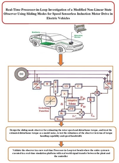
1. Introduction

Electric vehicles (EVs) have come to occupy considerable space in the transportation sector owing to less harmful emissions, better energy profile, lesser noise and cheaper maintenance and operating costs. However, disadvantages exist in the form of range anxiety, charging infrastructure and battery safety and disposal. An induction motor continues to dominate owing to its robustness, ruggedness, smaller size and plays a major role in the electric transportation domain [1,2]. Additionally, the speed range or bandwidth of the motor plays a major role in an EV. One major aspect, which has often been overlooked, is the space constraints inside the EV. Although the induction motor is compact and eliminates the use of commutator brush assembly (as seen in DC motors), the presence of the speed sensor mounted on the motor shaft adds to the space and additional electronics (sensitive to vehicle vibrations and dynamics) in the EV system. Therefore, it is felt that a sensorless speed estimation system is suitable and also economically and technologically feasible in an EV. Additionally, the use of the speed sensor also adds to the non-linearity of the system by means of the sensor noise, which may affect the gain and dynamic performance of the motor used in the EV [3]. The domain of speed sensorless estimation and control of induction motors has gained popularity for the past decade due to the elimination of the speed sensor owing to cost, reliability and sensitivity constraints [4]. Adaptive speed and parameter observation schemes became more popular owing to their pace of adaptation, ease of use and less computational space [5,6]. The decoupled control strategy also emerged as the most popular one [7,8]. Recently numerous controllers are proposed using wavelet transform and fuzzy tuning (WTFT) [9,10]. Computational intelligence based state estimation also added to the ongoing research on parameter estimation and online adaptation [11,12]. Most of the adaptive schemes follow the concept of model reference adaptive systems (MRASs) [13] as shown in Figure 1. Investigation particularly towards the different configuration schemes based on the state observers is also presented [14]. The extended Kalman filters are widely applied for state estimation, and demanded extensive computational space and a high sampling frequency [15]. Besides, the system dynamics can be linearized for the accuracy. Most of them focused on joint state estimation and adaptation at speeds ranging from low speeds to flux weakening regions [16,17]. Extended Luenberger observer (ELO) had an additional correction term [18] incorporated into the state dynamic equation, which involved the stator current error dynamics and provided more efficient dynamic and robust performance [19,20]. The variable structure concept [21] was also integrated into the ELO to constrain the system state and to reject the effect of the error dynamics, giving rise to sliding mode Luenberger observers (SMLOs) [22,23]. The very essence of observation schemes for the purpose of parameter estimation is brought about in [24]. Some investigations did focus on the estimation of disturbance as a parameter to test the robustness of the observer in offline simulation platforms [25,26]. The amount of non-linearities involved in a closed loop control system was brought about in [27]. Therefore, there was a need to decouple a non-linear system and control it in a linear domain. The emergence of power switching devices and the effect it had on variable frequency control was portrayed in [28]. This also had a negative effect in increasing the number of non-linearities in a drive system.

Presently, real-time validation platforms have taken over from offline simulation platforms. Several computer languages like Simulink and LabVIEW permit the creation of computer models, which can be connected to real-time embedded systems or electronic control units through digital and analog I/O (input/output) cards. There are many available in the market like xPC and Opal-RT’s RT-Lab along with real-time targets [29] that are primarily used for mechatronics, power electronics, electric vehicle drives and power grid protection tests. As part of the model based design strategy for testing computer models, there are several testing levels namely the software in loop (SIL), model in loop (MIL) and hardware in loop (HIL). While SIL is employed for verification of the code with respect to Matlab functions, MIL environment is used for testing the model without any physical hardware components. The PIL strategy is similar to MIL, however, there is a difference in signal routing that is real-time in PIL. Although several observers have been designed by making use of the concepts of sliding modes, artificial intelligence and model reference.

• Very few cater to the handling of measurement and model disturbances and their effects on the steady state and dynamic performance of the drive.
• Existing disturbance observers have short comings in terms of speed bandwidth, parameter estimation, torque profile and stability issues.
• Although many have been validated in an offline simulation platform, some in an experimental test bench, none of them have been tested in a real-time PIL test bench (which is an intermediate between offline simulation and full hardware verification).

The purpose of this work is to design, test and analyze a SMLO estimating the speed and disturbance torque for a three phase speed sensorless induction motor.

• By effective placement of the estimated disturbance torque in the proposed observer state dynamic equation, greater handling of the disturbance is seen as compared to the other disturbance observer whose tracking performance is affected. The speed bandwidth is increased and the torque holding capacity is also good. It is comparatively more stable and the dame has been analyzed through the pole placement technique.
• Furthermore, in a new real-time PIL platform, the plant and the controller are made to interact through digital and analog I/O cards by providing a real-time link. This testing is based on a model based design paradigm and has not been performed in the existing literature.

The paper is organized as follows: Section 1 relates to the motivation, literature survey and the limitations of the existing work and the key contributions of the paper. Section 2 discusses the basic principle of the adaptive system and the structure of the observer using sliding modes, the proposed disturbance rejection mechanisms inside the observers and the stability analysis of the conventional and proposed disturbance observers. Section 3 outlines the mathematical structure of the existing indirect vector control strategy. Section 4 focuses on an elaborate introduction and representation of the real-time test bench based on Opal-RT for the system validation. Section 5 presents the detailed results and analysis of the dynamic and static performance of the observers when subjected to different test cases followed by the pole placement study and performance comparison. Finally, the conclusion section emphasizes the importance of the findings to the existing literature and its significance with respect to vehicle performance and dynamics.

2. Basic Principle of MRAS and Structure of the SMLO

The SMLO with the estimated disturbance torque incorporated into the sliding hyperplane is shown in Figure 2a. It is a multiple input multiple output system (MIMO) where the inputs are the terminal quantities of the motor and the outputs are the estimated speed and the disturbance torque. The state space model of the motor and the observer are used, as it is suited for estimation and control functions. The primary reason of adaptive control is for parameter estimation. It is to match the desired performance (observer model) with that of the process (motor model). This principle can be explained as an optimization problem. Therefore, the essence is to minimize the error for state convergence. The complete system is shown in Figure 2b. Here, ‘A’ represents the system matrix, ‘^’ denotes estimated parameters, ‘X’ represents the state variables comprising of the d and q axes stator and currents rotor fluxes, ‘k_sw’ is the switching gain, it can either be a fixed value or a reduced order matrix. ‘J’, ‘p’ and ‘B_V’ represent the moment of inertia, differential operator and viscous friction coefficient respectively. ‘${\mathrm{T}}_{\mathrm{e}}^{*}$’ and ‘${\hat{\mathrm{T}}}_{\mathrm{dis}}$’ are electromagnetic and estimated disturbance torque, ‘k’ is a positive gain.

The selection and the stability conditions of the sliding hyperplane play a major role in observer dynamics. It should be selected such that it satisfies the Lyapunov stability criterion [30]. The sliding hyperplane ‘S’ and the LFC (Lyapunov function candidate) “V” is a scalar function of S [31].

$$\dot{\mathrm{V}}\left(\mathrm{S}\right)=\mathrm{S}\left(\mathrm{x}\right)\dot{\mathrm{S}}\left(\mathrm{x}\right)$$

(1)

The control law is expressed as:

$$\mathrm{u}\left(\mathrm{t}\right)={\mathrm{u}}_{\mathrm{e}\mathrm{q}}\left(\mathrm{t}\right)+{\mathrm{u}}_{\mathrm{s}\mathrm{w}}\left(\mathrm{t}\right)$$

(2)

The switching vector ${\mathrm{u}}_{\mathrm{sw}}\left(\mathrm{t}\right)$ satisfying stability conditions:

$${\mathrm{u}}_{\mathrm{sw}}\left(\mathrm{t}\right)=\mathsf{\eta }\mathrm{sign}\left(\mathrm{S}\left(\mathrm{x},\mathrm{t}\right)\right)$$

(3)

where, $\mathrm{sign}\left(\mathrm{S}\right)=\{\begin{array}{c}-1 \mathrm{for} \mathrm{S}<0\\ 0 \mathrm{for} \mathrm{S}=0\\ +1 \mathrm{for} \mathrm{S}>0\end{array}$, where, η denotes the switching control gain so as to make (1) negative definite. This implies:

$$\mathrm{S}\left(\mathrm{x}\right)\dot{\mathrm{S}}\left(\mathrm{x}\right)<0$$

(4)

This constrains the disturbance. Chattering is produced due to this non-linear high frequency switching. To remove it, a saturation function with boundary layer of width (Φ) replacing sign (S) with sat (S/Φ):

$$\mathrm{sat}\left(\mathrm{S}/\mathsf{\Phi }\right)=\{\begin{array}{c}\mathrm{sign}\left(\frac{\mathrm{S}}{\mathsf{\Phi }}\right)\mathrm{if} \left|\left(\frac{\mathrm{S}}{\mathsf{\Phi }}\right)\right|1\\ \left(\frac{\mathrm{S}}{\mathsf{\Phi }}\right)\mathrm{if} \left|\left(\frac{\mathrm{S}}{\mathsf{\Phi }}\right)\right|<1\end{array}$$

(5)

2.1. Motor Model (Reference)

$$\frac{\mathrm{d}\mathrm{x}}{\mathrm{d}\mathrm{t}}=\left[\mathrm{A}\right]\mathrm{x}+\left[\mathrm{B}\right]\mathrm{u}$$

(6)

$$\mathrm{y}=\left[\mathrm{C}\right]\mathrm{x}$$

(7)

where,

$$\mathrm{x}={\left[{\mathrm{i}}_{\mathrm{ds}}^{\mathrm{s}},{\mathrm{i}}_{\mathrm{qs}}^{\mathrm{s}},{\mathsf{\psi }}_{\mathrm{dr}}^{\mathrm{s}},{\mathsf{\psi }}_{\mathrm{qr}}^{\mathrm{s}}\right]}^{\mathrm{T}},\mathrm{A}=\left[\begin{array}{cc}{\mathrm{A}}_{11}& {\mathrm{A}}_{12}\\ {\mathrm{A}}_{21}& {\mathrm{A}}_{22}\end{array}\right]$$

$$\mathrm{B}={\left[\frac{1}{{\mathsf{\sigma }\mathrm{L}}_{\mathrm{s}}}\mathrm{I}0\right]}^{\mathrm{T}},\mathrm{C}=\left[\mathrm{I},0\right],\mathrm{u}={\left[{\mathrm{v}}_{\mathrm{ds}}^{\mathrm{s}}{\mathrm{v}}_{\mathrm{qs}}^{\mathrm{s}}\right]}^{\mathrm{T}}$$

$$\mathrm{I}=\left[\begin{array}{cc}1& 0\\ 0& 1\end{array}\right],\mathrm{J}=\left[\begin{array}{cc}0& -1\\ 1& 0\end{array}\right]$$

$${\mathrm{A}}_{11}=-\left[\frac{{\mathrm{R}}_{\mathrm{s}}}{{\mathsf{\sigma }\mathrm{L}}_{\mathrm{s}}}+\frac{1-\mathsf{\sigma }}{{\mathsf{\sigma }\mathrm{T}}_{\mathrm{r}}}\right]\mathrm{I}={\mathrm{a}}_{\mathrm{r}11}\mathrm{I}$$

$${\mathrm{A}}_{12}=\frac{{\mathrm{L}}_{\mathrm{m}}}{{\mathsf{\sigma }\mathrm{L}}_{\mathrm{s}}{\mathrm{L}}_{\mathrm{r}}}\left[\frac{1}{{\mathrm{T}}_{\mathrm{r}}}\mathrm{I}-{\mathsf{\omega }}_{\mathrm{r}}\mathrm{J}\right]={\mathrm{a}}_{\mathrm{r}12}\mathrm{I}+{\mathrm{a}}_{\mathrm{i}12}\mathrm{J}$$

$${\mathrm{A}}_{21}=\frac{{\mathrm{L}}_{\mathrm{m}}}{{\mathrm{T}}_{\mathrm{r}}}\mathrm{I}={\mathrm{a}}_{\mathrm{r}21}\mathrm{I}$$

$${\mathrm{A}}_{22}=\frac{-1}{{\mathrm{T}}_{\mathrm{r}}}\mathrm{I}+{\mathsf{\omega }}_{\mathrm{r}}\mathrm{J}={\mathrm{a}}_{\mathrm{r}22}\mathrm{I}+{\mathrm{a}}_{\mathrm{i}22}\mathrm{J}$$

2.2. Disturbance Torque Estimation

It is expressed as:

$${\hat{\mathrm{T}}}_{\mathrm{dis}}={\mathrm{T}}_{\mathrm{e}}^{*}-\mathrm{J}\frac{\mathrm{d}\hat{\mathsf{\omega }}}{\mathrm{dt}}-{\mathrm{B}}_{\mathrm{V}}\hat{\mathsf{\omega }}$$

(8)

2.3. SMLO1

The way the disturbances are handled play a major role in state convergence of an observer system. The disturbance handling method in SMLO1 is similar to many disturbance observers where the estimated disturbance is integrated into the state dynamic equation. In this case, the main difference from the proposed method (SMLO2) is the way it handles the disturbance. Here, it is not constrained in the sliding hyperplane. Therefore, the estimated disturbance is not part of the state convergence of the sliding hyperplane. This is elaborated in the following model:

$$\frac{\mathrm{d}\hat{\mathrm{x}}}{\mathrm{dt}}=\left[\hat{\mathrm{A}}\right]\hat{\mathrm{x}}+\left[\mathrm{B}\right]\mathrm{u}+{\mathrm{k}}_{\mathrm{sw}}\mathrm{sat}\left({\hat{\mathrm{i}}}_{\mathrm{s}}-{\mathrm{i}}_{\mathrm{s}}\right)+\hat{\mathrm{d}}$$

(9)

Sliding surface or hyperplane is $\mathrm{s}={\hat{\mathrm{i}}}_{\mathrm{s}}-{\mathrm{i}}_{\mathrm{s}}\mathrm{and}\hat{\mathrm{d}}={\mathrm{k}\hat{\mathrm{T}}}_{\mathrm{dis}}$

$$\hat{\mathrm{y}}=\left[\mathrm{C}\right]\hat{\mathrm{x}}$$

(10)

where ${\hat{\mathrm{i}}}_{\mathrm{s}},{\mathrm{i}}_{\mathrm{s}}$= estimated and actual stator currents.

$$\hat{\mathrm{A}}=\left[\begin{array}{cc}{\mathrm{A}}_{11}& {\hat{\mathrm{A}}}_{12}\\ {\mathrm{A}}_{21}& {\hat{\mathrm{A}}}_{22}\end{array}\right]$$

$${\hat{\mathrm{A}}}_{12}=\frac{{\mathrm{L}}_{\mathrm{m}}}{{\mathsf{\sigma }\mathrm{L}}_{\mathrm{s}}{\mathrm{L}}_{\mathrm{r}}}\left[\frac{1}{{\mathrm{T}}_{\mathrm{r}}}\mathrm{I}-{\hat{\mathsf{\omega }}}_{\mathrm{r}}\mathrm{J}\right]={\mathrm{a}}_{\mathrm{r}12}\mathrm{I}+{\hat{\mathrm{a}}}_{\mathrm{i}12}\mathrm{J}$$

$${\hat{\mathrm{A}}}_{22}=\frac{-1}{{\mathrm{T}}_{\mathrm{r}}}\mathrm{I}+{\hat{\mathsf{\omega }}}_{\mathrm{r}}\mathrm{J}={\mathrm{a}}_{\mathrm{r}22}\mathrm{I}+{\hat{\mathrm{a}}}_{\mathrm{i}22}\mathrm{J}$$

Using the reduced order matrix:

$${\mathrm{k}}_{\mathrm{sw}}={\left[\begin{array}{cc}{\mathrm{k}}_1& {\mathrm{k}}_2\\ -{\mathrm{k}}_2& {\mathrm{k}}_1\end{array}\right]}^{\mathrm{T}}$$

(11)

The purpose of the switching gain is to make (2) stable through pole placement. The eigenvalues of the observer must be more negative with respect to the motor for faster convergence of the observer and motor states. Consequently,

$${\mathrm{k}}_1=\left(\mathrm{m}-1\right){\mathrm{a}}_{\mathrm{r}11}$$

(12)

$${\mathrm{k}}_2={\mathrm{k}}_{\mathrm{p}},{\mathrm{k}}_{\mathrm{p}}\ge -1$$

(13)

Therefore, ‘m’ and ‘k₂’ are chosen to reflect the placement of the eigenvalues of the observer and the motor. Additionally, the dynamics and damping of the observer are affected by the same thing. ‘k₁’ is dependent on ‘m’ and motor parameters.

2.4. SMLO2

Here, the observer state dynamic equation is modified as shown:

$$\frac{\mathrm{d}\hat{\mathrm{x}}}{\mathrm{dt}}=\left[\hat{\mathrm{A}}\right]\hat{\mathrm{x}}+\left[\mathrm{B}\right]\mathrm{u}+{\mathrm{k}}_{\mathrm{sw}}\mathrm{sat}\left({\hat{\mathrm{i}}}_{\mathrm{s}}-{\mathrm{i}}_{\mathrm{s}}-\hat{\mathrm{d}}\right)$$

(14)

where, the sliding surface or hyperplane is $\mathrm{s}={\hat{\mathrm{i}}}_{\mathrm{s}}-{\mathrm{i}}_{\mathrm{s}}-\hat{\mathrm{d}}$ and $\hat{\mathrm{d}}={\mathrm{k}\hat{\mathrm{T}}}_{\mathrm{dis}}$

$$\hat{\mathrm{y}}=\left[\mathrm{C}\right]\hat{\mathrm{x}}$$

(15)

2.5. Adaptive Mechanism with LFC

It is denoted by M:

$$\mathrm{M}={\mathrm{e}}^{\mathrm{T}}\mathrm{e}+\frac{{\left({\hat{\mathsf{\omega }}}_{\mathrm{r}}-{\mathsf{\omega }}_{\mathrm{r}}\right)}^2}{\mathsf{\lambda }}$$

(16)

‘λ’, being, a positive constant.

The derivative of the function candidate with respect to t:

$$\frac{\mathrm{dM}}{\mathrm{dt}}={\mathrm{e}}^{\mathrm{T}}\left[{\left(\mathrm{A}+{\mathrm{k}}_{\mathrm{sw}}\mathrm{C}\right)}^{\mathrm{T}}+\left(\mathrm{A}+{\mathrm{k}}_{\mathrm{sw}}\mathrm{C}\right)\right]\mathrm{e}-\frac{2{\mathsf{\Delta }\mathsf{\omega }}_{\mathrm{r}}\left({\mathrm{e}}_{\mathrm{ids}}{\hat{\mathsf{\phi }}}_{\mathrm{qr}}^{\mathrm{s}}-{\mathrm{e}}_{\mathrm{iqs}}{\hat{\mathsf{\phi }}}_{\mathrm{dr}}^{\mathrm{s}}\right)}{\mathrm{c}}+\frac{2{\mathsf{\Delta }\mathsf{\omega }}_{\mathrm{r}}}{\mathsf{\lambda }}\frac{{\mathrm{d}\hat{\mathsf{\omega }}}_{\mathrm{r}}}{\mathrm{dt}}$$

(17)

where, ${\mathrm{e}}_{\mathrm{ids}}={\mathrm{i}}_{\mathrm{ds}}^{\mathrm{s}}-{\hat{\mathrm{i}}}_{\mathrm{ds}}^{\mathrm{s}}$ and ${\mathrm{e}}_{\mathrm{iqs}}={\mathrm{i}}_{\mathrm{qs}}^{\mathrm{s}}-{\hat{\mathrm{i}}}_{\mathrm{qs}}^{\mathrm{s}}$

From (16), the estimated speed expression is obtained.

$$\frac{{\mathrm{d}\hat{\mathsf{\omega }}}_{\mathrm{r}}}{\mathrm{dt}}=\frac{\mathsf{\lambda }}{\mathrm{c}}({\mathrm{e}}_{\mathrm{ids}}{\hat{\mathsf{\phi }}}_{\mathrm{qr}}^{\mathrm{s}}-{\mathrm{e}}_{\mathrm{iqs}}{\hat{\mathsf{\phi }}}_{\mathrm{dr}}^{\mathrm{s}})$$

(18)

‘c’ is arbitrary positive.

2.6. Stability Analysis by the Pole Placement Technique—SMLO1 and SMLO2

For the SMLO1 with conventional disturbance rejection mechanism, we have:

$$\left({\mathrm{A}}_{11}+{\mathrm{k}}_{\mathrm{sw}}+\hat{\mathrm{d}}\right)=\left[\begin{array}{cc}{\mathrm{a}}_{\mathrm{r}11}+{\mathrm{k}}_1+\hat{\mathrm{d}}& -{\mathrm{k}}_2+\hat{\mathrm{d}}\\ {\mathrm{k}}_2+\hat{\mathrm{d}}& {\mathrm{a}}_{\mathrm{r}11}+{\mathrm{k}}_1+\hat{\mathrm{d}}\end{array}\right]$$

(19)

Now, the characteristic equation can be obtained by:

$$\mathrm{SI}-\left({\mathrm{A}}_{11}+{\mathrm{k}}_{\mathrm{sw}}+\hat{\mathrm{d}}\right)=0$$

(20)

On solving, we get the characteristic equation of SMLO1:

$${\mathrm{S}}^2-2\mathrm{S}\left({\mathrm{a}}_{\mathrm{r}11}+{\mathrm{k}}_1+\hat{\mathrm{d}}\right)+{\left({\mathrm{a}}_{\mathrm{r}11}+{\mathrm{k}}_1+\hat{\mathrm{d}}\right)}^2+\left({\mathrm{k}}_2^2-{\hat{\mathrm{d}}}^2\right)=0$$

(21)

From the characteristic equation, the observer poles are obtained:

$${\mathrm{S}}_1=\left({\mathrm{a}}_{\mathrm{r}11}+{\mathrm{k}}_1+\hat{\mathrm{d}}\right)+\mathrm{j}\left({\mathrm{k}}_2-\hat{\mathrm{d}}\right)$$

(22)

$${\mathrm{S}}_2=\left({\mathrm{a}}_{\mathrm{r}11}+{\mathrm{k}}_1+\hat{\mathrm{d}}\right)-\mathrm{j}\left({\mathrm{k}}_2-\hat{\mathrm{d}}\right)$$

(23)

For the SMLO2 with improved disturbance rejection mechanism, we have:

$$\left({\mathrm{A}}_{11}+{\mathrm{k}}_{\mathrm{sw}}-{\mathrm{k}}_{\mathrm{sw}}\hat{\mathrm{d}}\right)=\left[\begin{array}{cc}{\mathrm{a}}_{\mathrm{r}11}+{\mathrm{k}}_1-{\mathrm{k}}_{\mathrm{sw}}\hat{\mathrm{d}}& -{\mathrm{k}}_2-{\mathrm{k}}_{\mathrm{sw}}\hat{\mathrm{d}}\\ {\mathrm{k}}_2-{\mathrm{k}}_{\mathrm{sw}}\hat{\mathrm{d}}& {\mathrm{a}}_{\mathrm{r}11}+{\mathrm{k}}_1-{\mathrm{k}}_{\mathrm{sw}}\hat{\mathrm{d}}\end{array}\right]$$

(24)

The characteristic equation is obtained by:

$$\mathrm{SI}-\left({\mathrm{A}}_{11}+{\mathrm{k}}_{\mathrm{sw}}-{\mathrm{k}}_{\mathrm{sw}}\hat{\mathrm{d}}\right)=0$$

(25)

Therefore, on solving, the characteristic equation of SMLO2:

$${\mathrm{S}}^2-2\mathrm{S}({\mathrm{a}}_{\mathrm{r}11}+{\mathrm{k}}_1-{\mathrm{k}}_{\mathrm{sw}}\hat{\mathrm{d}})+{\left({\mathrm{a}}_{\mathrm{r}11}+{\mathrm{k}}_1-{\mathrm{k}}_{\mathrm{sw}}\hat{\mathrm{d}}\right)}^2+\left({\mathrm{k}}_2^2-{\mathrm{k}}_{\mathrm{sw}}^2{\hat{\mathrm{d}}}^2\right)=0$$

(26)

The observer poles are obtained as follows:

$${\mathrm{S}}_1=\left({\mathrm{a}}_{\mathrm{r}11}+{\mathrm{k}}_1-{\mathrm{k}}_{\mathrm{sw}}\hat{\mathrm{d}}\right)+\mathrm{j}\left({\mathrm{k}}_2-{\mathrm{k}}_{\mathrm{sw}}\hat{\mathrm{d}}\right)$$

(27)

$${\mathrm{S}}_1=\left({\mathrm{a}}_{\mathrm{r}11}+{\mathrm{k}}_1-{\mathrm{k}}_{\mathrm{sw}}\hat{\mathrm{d}}\right)-\mathrm{j}\left({\mathrm{k}}_2-{\mathrm{k}}_{\mathrm{sw}}\hat{\mathrm{d}}\right)$$

(28)

3. Indirect Vector Control Strategy—Mathematical Structure

The pulse width modulation (PWM) technique employed here is hysteresis band current control as it has short circuit current protection feature, load independent and good torque response. A discrete PI controller processes and generates the reference torque.

$${\mathrm{e}}_{\mathrm{c}}={\widehat{\mathsf{\omega }}}_{\mathrm{r}}-{\mathsf{\omega }}^{*}$$

(29)

$${\mathrm{T}}_{\mathrm{e}}^{*}={\mathrm{e}}_{\mathrm{c}}\left[{\mathrm{k}}_{\mathrm{p}}+({\mathrm{k}}_{\mathrm{i}}/\mathrm{s})\ast {\mathrm{T}}_{\mathrm{s}}\right]$$

(30)

where, e_c, k_p, k_i and T_s denote speed error, proportional and integral gains and sampling time for control algorithm execution.

$${\mathrm{i}}_{\mathrm{ds}}{}^{*}=\left(\frac{{\mathsf{\psi }}_{\mathrm{r}}}{{\mathrm{L}}_{\mathrm{m}}}\right)\left[1+\frac{{\mathrm{dT}}_{\mathrm{r}}}{{\mathrm{dT}}_{\mathrm{s}}}\right]$$

(31)

$${\mathrm{i}}_{\mathrm{qs}}{}^{*}=\left(\frac{2}{3}\right)\left(\frac{2}{\mathrm{P}}\right)\left(\frac{{\mathrm{L}}_{\mathrm{r}}}{{\mathrm{L}}_{\mathrm{m}}}\right)\left(\frac{{\mathrm{T}}_{\mathrm{ref}}}{{\mathsf{\psi }}_{\mathrm{r}}}\right)$$

(32)

Stator current components are inversely transformed from synchronously rotating to three phases stationary reference frame making use of the field angle. Therefore, it is obtained from the slip speed, as shown:

$${\mathsf{\theta }}_{\mathrm{f}}={\mathsf{\theta }}_{\mathrm{sl}}+{\mathsf{\theta }}_{\mathrm{r}}$$

(33)

$${\mathrm{i}}_{\mathrm{as}}^{*}={\mathrm{i}}_{\mathrm{ds}}\sin \mathsf{\theta }+{\mathrm{i}}_{\mathrm{qs}}\cos \mathsf{\theta }$$

(34)

$${\mathrm{i}}_{\mathrm{bs}}^{*}=\left(\frac{1}{2}\right)\left\{-{\mathrm{i}}_{\mathrm{ds}}\cos \mathsf{\theta }+\surd 3{\mathrm{i}}_{\mathrm{ds}}\sin \mathsf{\theta }\right\}+\left(\frac{1}{2}\right)\left\{{\mathrm{i}}_{\mathrm{qs}}\sin \mathsf{\theta }+\surd 3{\mathrm{i}}_{\mathrm{qs}}\cos \mathsf{\theta }\right\}$$

(35)

$${\mathrm{i}}_{\mathrm{cs}}^{*}=-\left({\mathrm{i}}_{\mathrm{as}}^{*}+{\mathrm{i}}_{\mathrm{bs}}^{*}\right)$$

(36)

The generated currents and the actual sensed three phase currents are compared and the current errors are fed to the hysteresis band regulator to generate the switching pulses for the inverter. The hysteresis band value is chosen taking into account the torque and the current pulsations.

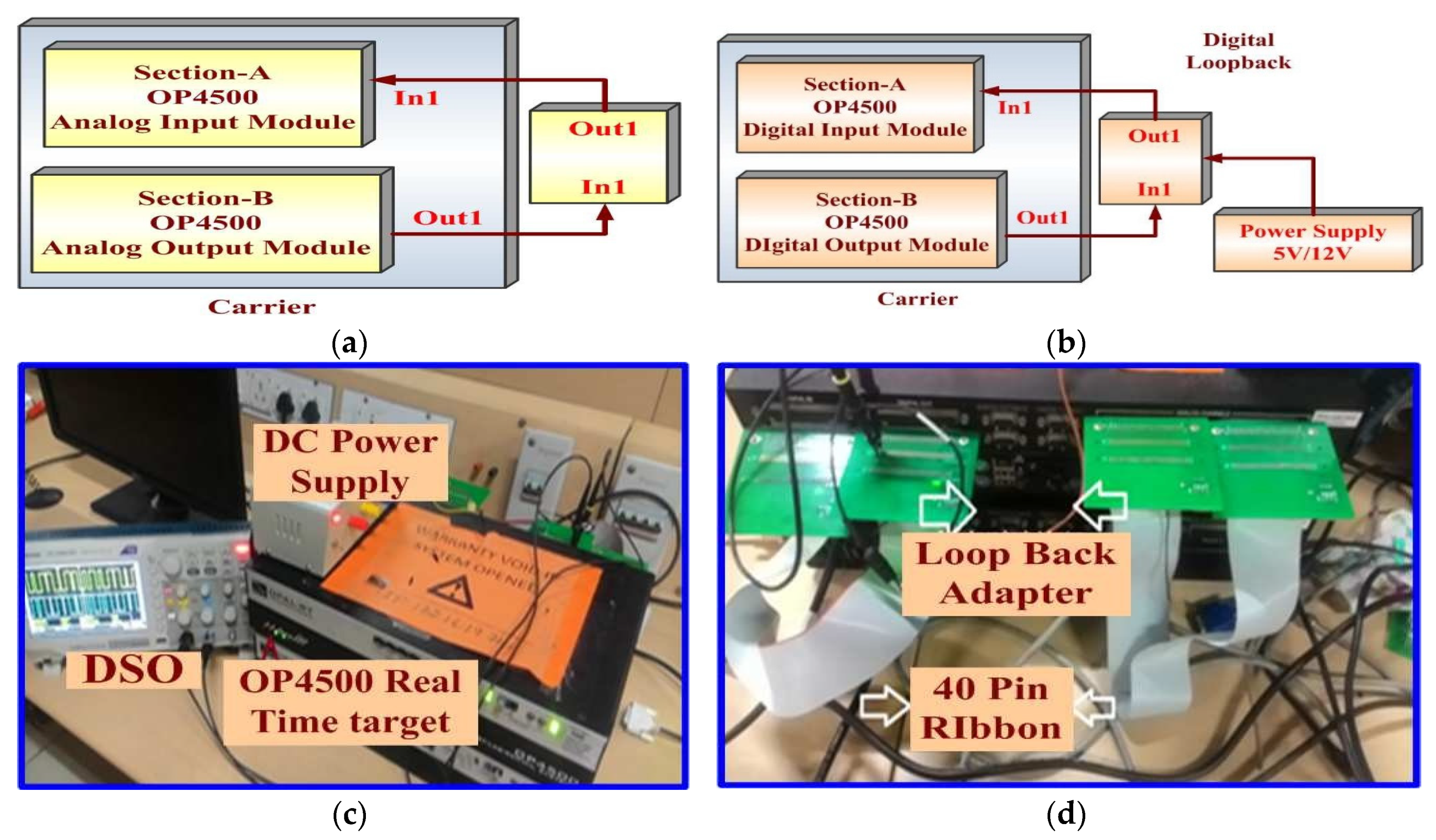
4. RT-Lab Based PIL Test Bench

Time critical test and simulation platforms have gained more prominence over offline platforms owing to faster execution, reduced design and development time. They use a fixed step discrete time solver compared to the variable step solvers used in offline. The computer model executed by them is in actual clock time provided the non-linearities and system dynamics are mathematically modeled. It has several features such as hardware-in-Loop testing (HIL), virtual and real control prototyping, data logging, etc. The sensorless drive system built using Simulink blocksets is integrated with RT-Lab blocksets [32,33]. However, the interaction between the plant and the controller is through analog and digital output and input channels and not by Simulink wires. Instead, a real-time link in the form of two loopback adapters along with a 40 pin flat ribbon cable is provided to ensure a real signal interaction. In this real-time link, only signal routing takes place, the signal is not processed. Therefore the estimated speed and actual 3 phase currents are fed via the analog output channels to the controller where it is captured by analog input channels. The switching pulses from the controller is sent via the digital output channels and captured by the digital input channels at the plant side. The output and the input pins and the number of channels are configured accordingly. This is also known as PIL testing [34,35]. The analog loopback is standalone hardware equipment, which does not need a power supply. A +5 V or +12 V source is required for Vsource and Vref for digital feedback. The operation of both of them are shown in the following schematic in Figure 3a,b. Two carriers are used as real-time targets. The OP4500 target has a single processor core activated. The OP5600 target has more processor cores, which makes it possible to have both the plant and controller in two different RT-Lab subsystems. The system model in the PC is connected to the OP4500/OP5600 targets through TCP/IP. The entire real-time test bench used for PIL testing is shown in Figure 3c,d for OP4500 and in Figure 4 for OP5600 target.

5. Results (Real-Time Simulation and PIL Based Validation): Analysis and Discussion

The time step used for the discretized model was 50 µs. Both the plant disturbance and the measurement disturbance were introduced in the system. The model was built in Simulink, interfaced with RT-Lab blocksets and the code generated was loaded and executed by the real-time target OP4500. Data logging was done by having OpWritefile blocksets of RT-lab to ensure the real-time data gets populated in mat files from where the real-time results can be extracted. Additionally, the estimated speed (analog output) and the switching pulses (digital output) were extracted from an oscilloscope to emphasize and validate (Hardware verification) the signal routing taking place between the plant and the controller via the Loopback adapter and cables. For, the study, a three-phase, 415 V, 50 Hz, star connected, 4 pole induction motor with the following model parameters considered are given below in

Table 1. Model parameters.

Parameters	Ratings
Rated Power	50 HP
Rated Load Torque	237.4 Nm
Rs	0.087 Ω
Rr	0.228 Ω
Lls	0.8 mH
Llr	0.8 mH
Lm	34.7 mH
Inertia, J	1.662 kg m2
Friction factor	0.1

.

Both observers were analyzed in terms of their dynamic performance, like tracking ability, disturbance rejection, speed bandwidth, time domain responses like overshoot, etc. Load perturbations and speed command variations could also be considered as model disturbances. The dynamic performance was obtained for the following test cases.

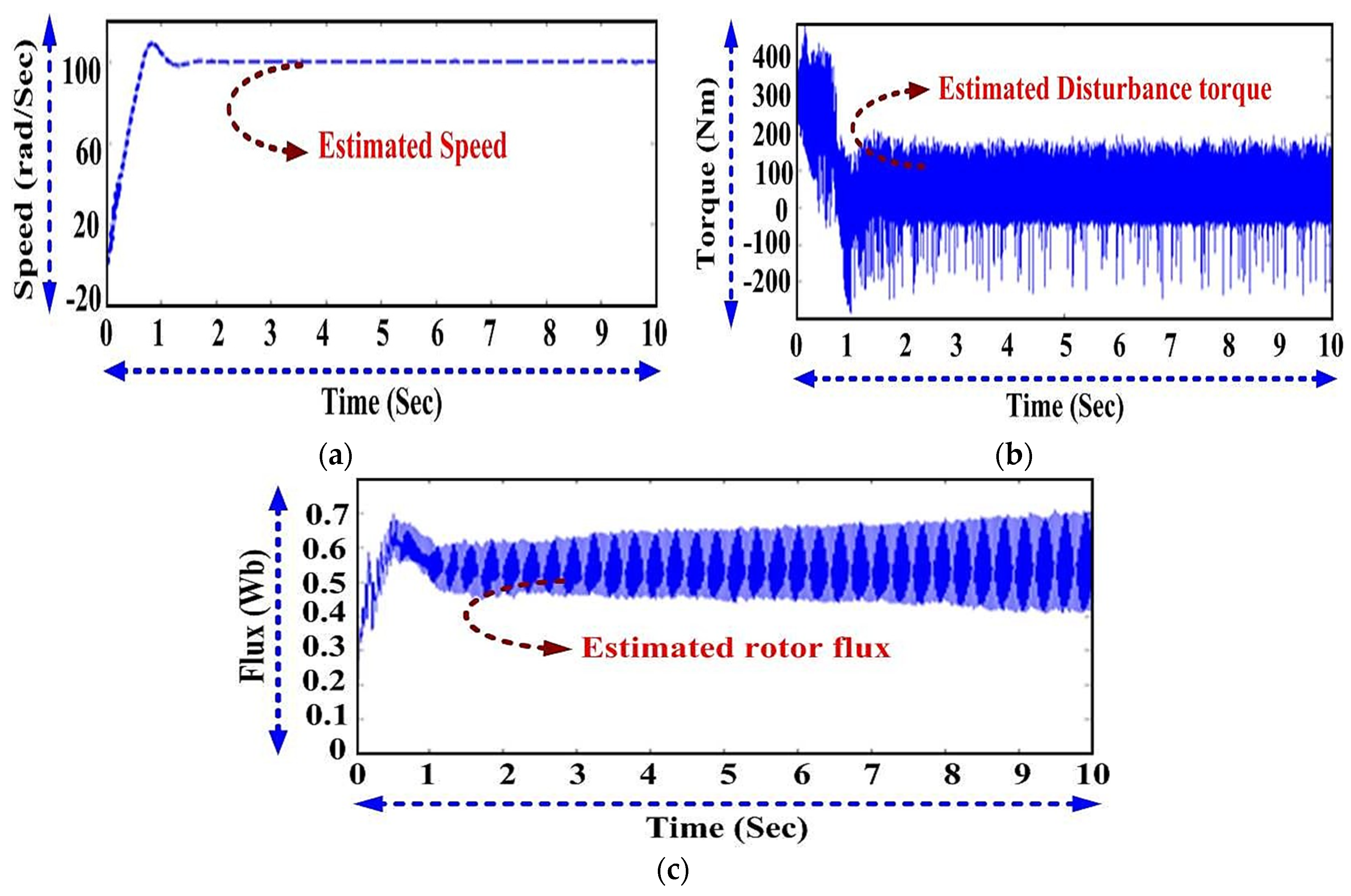
5.1. A Constant Speed Reference of 100 rad/s with a Constant Load Perturbation of 100 Nm

Both the observers are validated and analysed accordingly in the below subsections. For a constant speed command and load, both observers SMLO1 and SMLO2 exhibited similar tracking. The estimated speed, disturbance torque and rotor flux of both the observers were similar at medium speeds. The oscillations in speed tracking and the overshoot were tolerable.

5.1.1. SMLO1

The tracking performance of SMLO1 and the dynamic performance of the same in terms of torque holding capability and flux levels is shown in Figure 5.

5.1.2. SMLO2

The tracking performance of SMLO2 and the dynamic performance of the same in terms of torque holding capability and flux levels is shown in Figure 6.

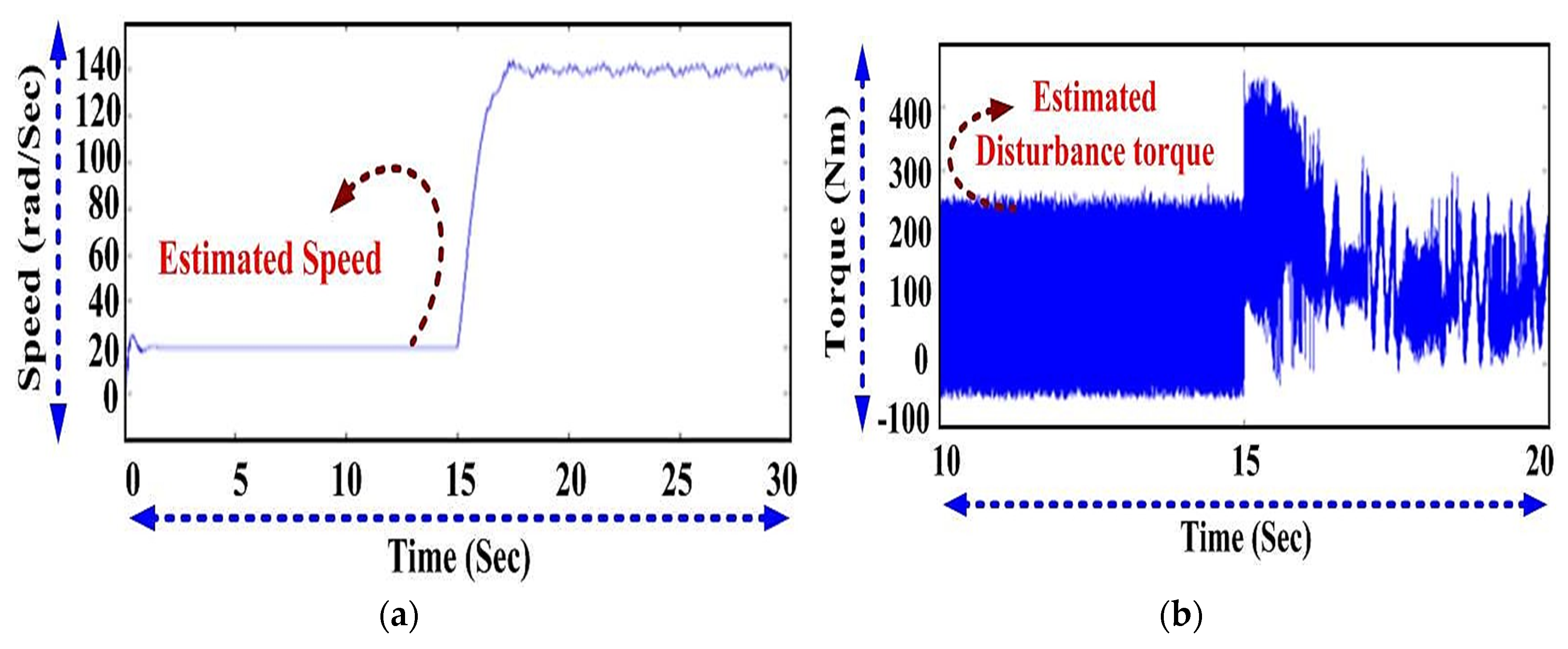
5.2. A Constant Speed Reference of 100 rad/s with a Step Load Perturbation (Initially at 5 Nm, after a Fixed Time Interval of 15 s, Stepped up to 200 Nm)

Even when the drive was subjected to sudden load step perturbation from light load to rated load, the performance at medium speeds for both the observers were similar. However, there was a slight variation in the estimated flux performance of SMLO2 over SMLO1. The estimated flux of the former stabilized after the load switched to the rated load. This could be attributed to better torque holding capability of the improved disturbance rejection mechanism.

5.2.1. SMLO1

The tracking performance of SMLO1 and the dynamic performance of the same in terms of torque holding capability and flux levels is shown in Figure 7.

5.2.2. SMLO2

The tracking performance of SMLO2 and the dynamic performance of the same in terms of torque holding capability and flux levels is shown in Figure 8.

5.3. A Step Speed Reference with a Constant Load Perturbation of 100 Nm

The difference is observed here when a step speed command is given. Additionally, there were some oscillations present initially when SMLO1 was tracking at 40 rad/s. As compared, the SMLO2 tracked well at speeds as low as 20 rad/s with considerably very few oscillations. The inability to track lower speeds may be due to the state convergence going out of bounds due to magnification of the speed and the stator current errors and also mismatch in critical parameters such as stator resistance, rotor time constant, etc. The flux pulsations were slightly more in SMLO1 as compared to SMLO2 and their profiles were different at low and medium speeds. However, the estimated disturbance torque of both were almost similar due to similar torque error between the motor and the observer errors in SMLO1 and SMLO2, however, the speed bandwidth varied.

5.3.1. SMLO1

The tracking performance of SMLO1 and the dynamic performance of the same in terms of torque holding capability and flux levels is shown in Figure 9.

5.3.2. SMLO2

The tracking performance of SMLO2 and the dynamic performance of the same in terms of torque holding capability and flux levels is shown in Figure 10.

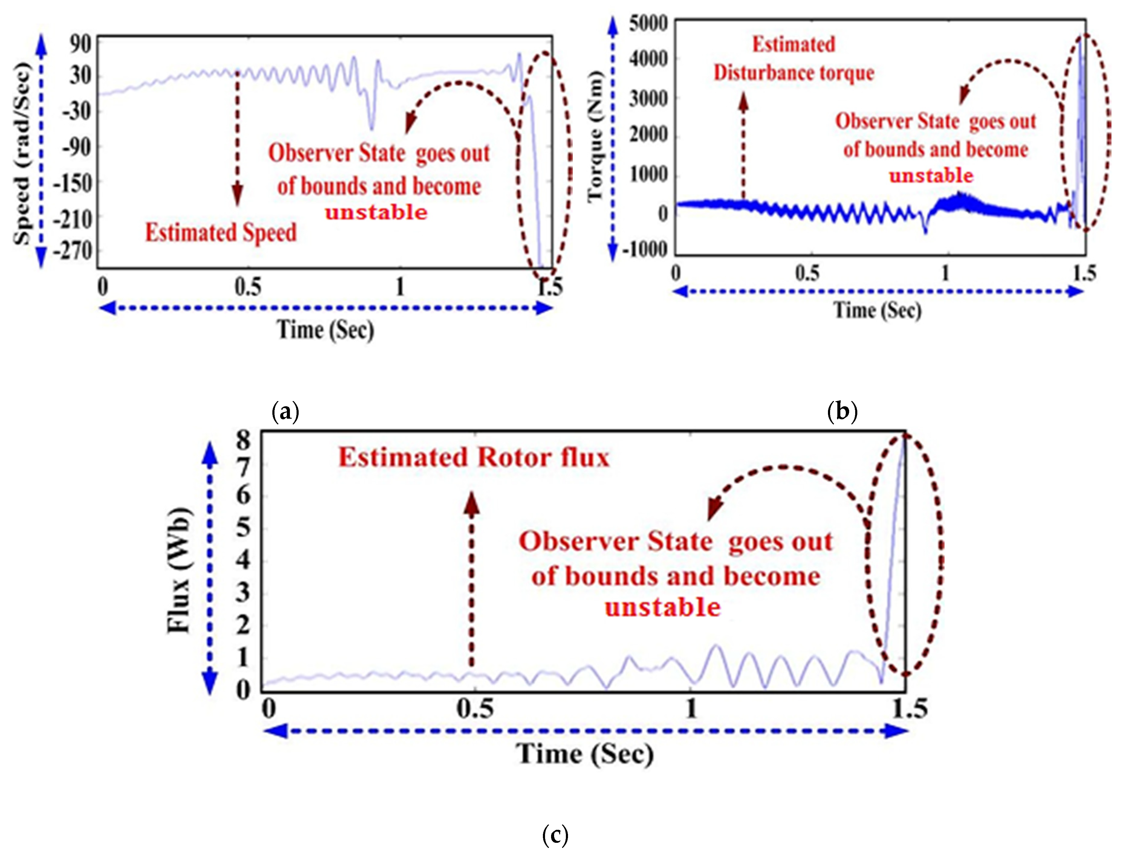
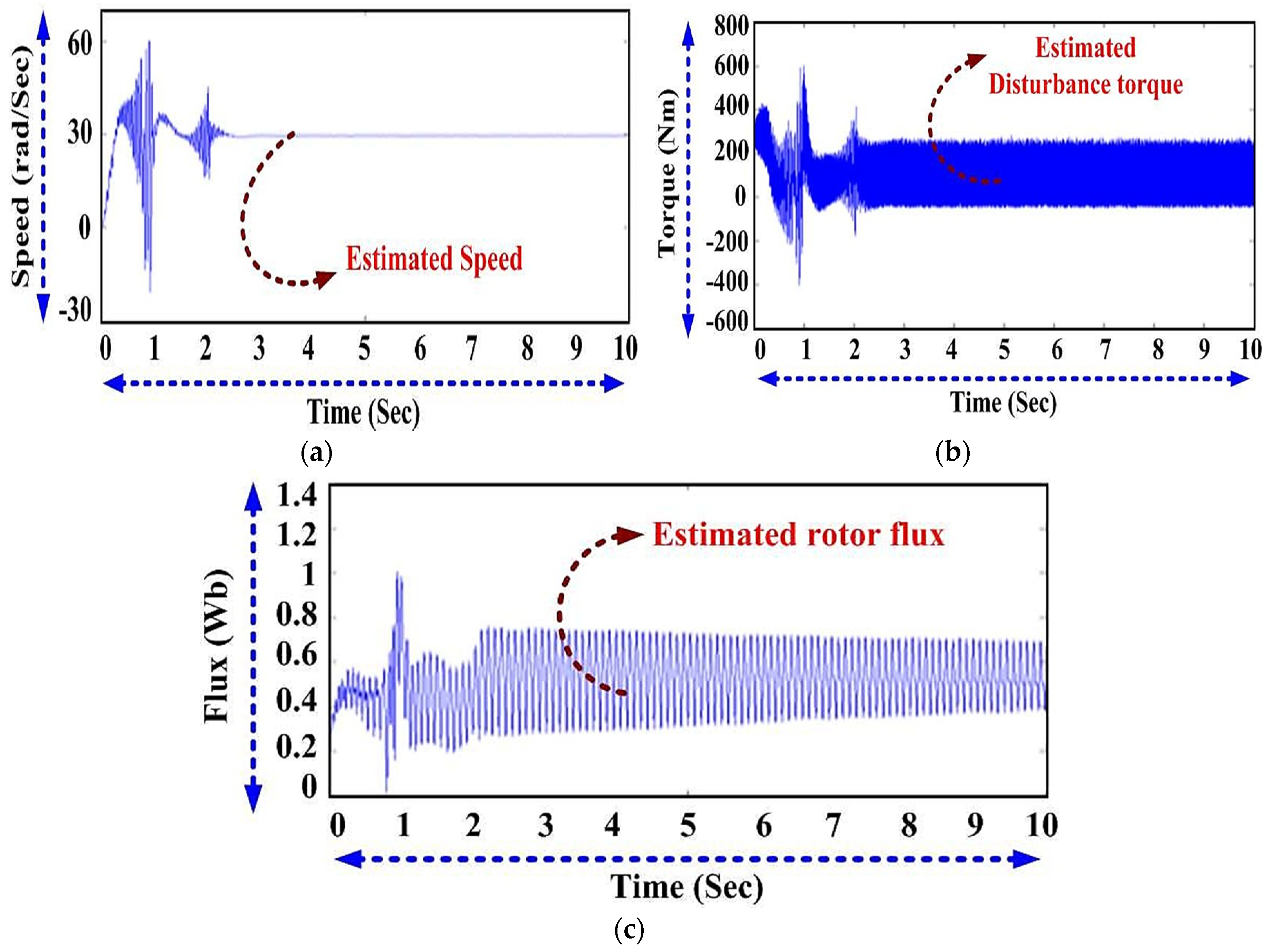
5.4. Low Speed Command of 30 rad/s with a Constant Load Perturbation of 100 Nm

To verify, the low speed state convergence of both the observers, they were subjected to a low speed command of 30 rad/s at constant load.

5.4.1. SMLO1

It can be clearly seen for SMLO1 in Figure 11 that around a time interval of 1.5 s, all the parameters went out of bounds and became unstable. This only reflected the mismatch in parameter and error dynamics at low speeds.

5.4.2. SMLO2

Analysis Case 1: Real Time Simulation with Processor-in-Loop Validation

Here, for the purpose of adding more weight to the findings, the low speed performance analysis was split into two cases. In case 1, the low speed performance was validated in the real time processor-in-loop platform as was done for all the previous test cases. It can be observed that in analysis case 1, for SMLO2, in spite of the initial high overshoot and undershoot present for a short interval of time in the estimated speed, after 3 s, it settled down and provided a smooth tracking, which is also reflected in the disturbance torque and the estimated flux waveforms shown in Figure 12.

In analysis case 2, only the low speed performance of the SMLO2 was considered, and an additional fragment for a time period of 4.5–5.5 s was zoomed for the purpose of clarity. Here, the same was tested in just the real time simulation environment (without the processor-in-loop mode). Here, the loop back cables, adapter and the power supply for the same was removed. Although the model was executed in real-time, however, there was no real world signal interaction between the plant and the controller here.

Analysis Case 2: Real Time Simulation without Processor-in-Loop Validation

It can be seen in Figure 13 that the number of overshoots and undershoots were considerably reduced as compared to analysis case 1 and in the additional zoomed fragment of the speed waveform, the tracking performance was very good with a bandwidth ranging from 29.95 to 30.05 rad/s, which only proved the effectiveness of the same in the low speed region.

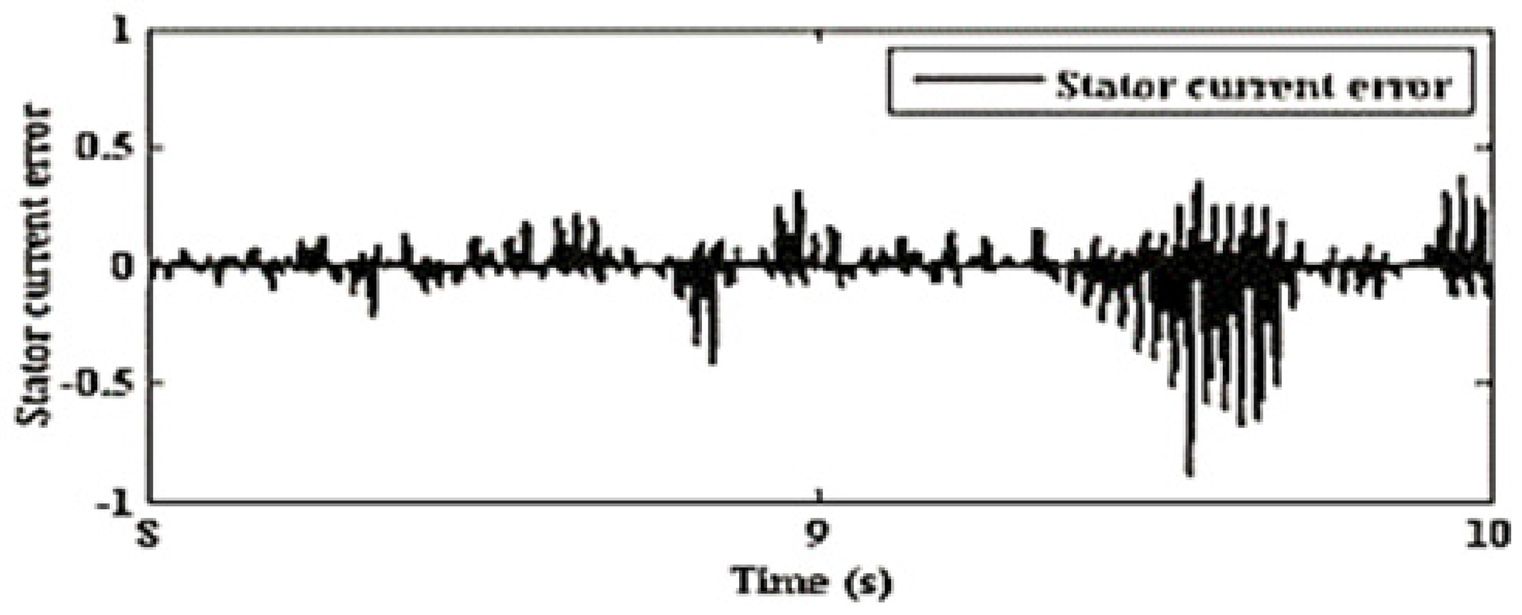
5.4.3. SMLO1 and SMLO2 Stator Current Error Convergence

The high torque pulsations (estimated disturbance torque) were due to high pulsations in the stator current. The large stator current pulsations and the subsequent stator current error was converged well by the SMLO2 as compared to SMLO1, as shown in Figure 14 and Figure 15.

5.5. Estimated Speed Waveforms for a Constant Load Perturbation of 100 Nm as Recorded in Digital Storage Oscilloscope

The estimated speed for different speed commands from the oscilloscope is shown in Figure 16a–d.

The poles of SMLO2 were shifted to the left of SMLO1 as shown in Figure 17 indicating improved stability performance. The effect of this was more predominant in the low speed regions where the SMLO2 was able to track speeds around 20 rad/s as compared to SMLO1, which is unable to track speeds of the same range. The poles being shifted more to the left of SMLO1 had led to increased speed bandwidth of SMLO2. Owing to high rating of the motor, the dynamics of the stator current impacted the performance of the observer and as a result, the pulsations in the disturbance torque could be attributed to the same. For hysteresis regulation, it is difficult to predict the exact switching frequency since it is not related to the hysteresis band. The OP45OO target provides a maximum switching frequency of (1/(2 × time step)), i.e., 10 kHz. Owing to successful execution of the model, it is to be understood that the switching frequency was within the 10 kHz range. Driving an EV is an endless series of dynamically changing operating states corresponding to the actual driving trajectory and speed of the vehicle, however, the analysis confines itself to low and medium speeds in the motoring mode and for constant load torque of 100 Nm (for all cases except Section 5.2, where there is a step load perturbation).

Table 2. Performance comparison.

Parameters	SMLO1	SMLO2 (Proposed)
Medium speeds and near synchronous speed (70–150 rps)	Exhibits good tracking performance	Exhibits good tracking performance
Low speeds (<70 rps)	Convergence is affected and does not track well.	Tracks up to 20 rps and considerably better disturbance rejection.
Speed oscillations	Has more oscillations even in the steady state region	Comparatively less oscillations
Observer stability	Less stable than the proposed observer, due to which the speed bandwidth is reduced.	Proposed observer poles are shifted to the left of the SMLO1, which explains the extended speed bandwidth.

highlights the improved dynamic performance of the proposed observer for the different parameters.

6. Conclusions

The two sliding mode observers with different disturbance rejection mechanisms (SMLO1 and SMLO2) for speed sensor-less induction motor drives were designed, tested and analyzed in a new real-time Processor-in-Loop test bench based on a distributed real-time package RT-Lab for application in the EV.

• The purpose of validating the same in a Processor-in-Loop platform is to introduce a real-world signal routing and interaction where the system is placed virtually in the front end.
• The dynamic performance can be treated almost on par with an actual physical system with precise timing requirements.
• SMLO2 displays better performance at low speed regions (less than 70 rps), particularly in terms of tracking, better disturbance handling and stability.
• It also has increased speed bandwidth (20–150 rps) and reduced speed oscillations at lower speeds (20–30 rps).
• The proposed method (SMLO2) would be more ideal for the EV to address the issue of range anxiety. It also delivers considerably better dynamic performance and able to handle disturbances better.

However, it can be further modified considering the real-time trajectory of the EV. This method of hardware verification can also be further extended to having the real world controller interact with the virtual plant or vice versa, where the real plant can interact with the virtual controller placed in the target.

References

- Tomislav, S.; Siegfried, S.; Wolfgang, G. The Flux-Based Sensorless Field-Oriented Control of Permanent Magnet Synchronous Motors without Integrational Drift. Actuators 2018, 7, 1–22. [Google Scholar]
- Tsuji, M.; Chen, S.; Izumi, K.; Yamada, E. A Sensorless Vector Control System for Induction Motors Using q-Axis Flux with Stator Resistance Identification. IEEE Trans. Ind. Electron. 2001, 48, 185–194. [Google Scholar] [CrossRef]
- Wang, H.; Liu, Y.C.; Ge, X. Sliding-mode observer-based speed-sensorless vector control of linear induction motor with a parallel secondary resistance online identification. IET. Electr. Power Appl. 2018, 12, 1215–1224. [Google Scholar] [CrossRef]
- Hosseyni, A.; Trabelsi, R.; Mimouni, M.F.; Iqbal, A.; Padmanaban, S. Novel Sensorless Sliding Mode Observer of a Five-Phase Permanent Magnet Synchronous Motor Drive in Wide Speed Range. Lect. Notes Electr. Eng. 2017, 436, 213–220. [Google Scholar]
- Hosseyni, A.; Trabelsi, R.; Iqba, A.; Padmanaban, S.; Mimouni, M. An Improved Sensorless Sliding Mode Control/ Adaptive Observer of a Five-Phase Permanent Magnet Synchronous Motor Drive. Int. J. Adv. Manuf. Tech. 2017, 93, 1029–1039. [Google Scholar] [CrossRef]
- Krishna, S.M.; Daya, J.L.F. Effect of Parametric variations and Voltage Unbalance on Adaptive Speed Estimation Schemes for Speed Sensorless Induction Motor Drives. Int. J. Power Electron. Drives. 2015, 6, 77–85. [Google Scholar] [CrossRef]
- Ali Karami, M.; Hamed, T. Estimation of load torque in induction motors via dynamic sliding mode control and new nonlinear state observer. J. Mech. Sci. Technol. 2018, 32, 2283–2288. [Google Scholar] [CrossRef]
- Alexander, I.K.; Alexey, A.E.; Dmitriy, V.S.; Yuriy, N.K. An Approach of the Wavelet-Fuzzy Controller of Vector Control System by the Induction Motor. In Proceedings of the IEEE International Multi-Conference on Industrial Engineering and Modern Technologies (FarEastCon), Vladivostok, Russia, 3–4 October 2018; pp. 1–6. [Google Scholar]
- Ho, T.J.; Chang, C.H. Robust Speed Tracking of Induction Motors: An Arduino-Implemented Intelligent Control Approach. Appl. Sci. 2018, 8, 159. [Google Scholar] [CrossRef]
- Zhao, X.; Yu, Q.; Yu, M.; Tang, Z. Research on an equal power allocation electronic differential system for electric vehicle with dual-wheeledmotor front drive based on a wavelet controller. Adv. Mech. Eng. 2018, 10, 1–24. [Google Scholar] [CrossRef]
- Bouhoune, K.; Yazid, K.; Boucherit, M.S.; Chriti, A. Hybrid control of the three phase induction machine using artificial neural networks and fuzzy logic. Appl. Soft Comput. 2017, 55, 289–301. [Google Scholar] [CrossRef]
- Daya, J.L.F.; Padmanaban, S.; Blaabjerg, F.; Wheeler, P.; Ojo, O. Implementation of Wavelet Based Robust Differential Control for Electric Vehicle Application. IEEE Trans. Power Electr. 2015, 30, 6510–6513. [Google Scholar] [CrossRef]
- Chekroun, S.; Zerikat, M.; Mechernene, A.; Benharir, N. Novel Observer Scheme of Fuzzy-MRAS Sensorless Speed Control of Induction Motor Drive. J. Phys. Conf. 2017, 783, 1–13. [Google Scholar] [CrossRef]
- Lamia, Y.; Sebti, B.; Farid, N.; Mihai, C.; Luis Guasch, P. Design of an Adaptive Fuzzy Control System for Dual Star Induction Motor Drives. Adv. Electr. Comput. Eng. 2018, 18, 37–44. [Google Scholar]
- Krisztián, H.; Márton, K. Speed sensorless field oriented control of induction machines using unscented Kalman filter. In Proceedings of the International Conference on Optimization of Electrical and Electronic Equipment (OPTIM) & Intl Aegean Conference on Electrical Machines and Power Electronics (ACEMP), Brasov, Romania, 25–27 May 2017; pp. 523–528. [Google Scholar]
- Bo, F.; Zhumu, F.; Leipo, L.; Jiangtao, F. The full-order state observer speed-sensorless vector control based on parameters identification for induction motor. Meas. Control 2019, 52, 202–211. [Google Scholar]
- Ali, H.; Rachid, D.; Othman, H. A New Direct Speed Estimation and Control of the Induction Machine Benchmark: Design and Experimental Validation. Math. Probl. Eng. 2018, 2018, 1–10. [Google Scholar]
- Krishna, S.M.; Daya, J.L.F.; Padmanaban, S.; Mihet-Popa, L. Real-time Analysis of a Modified State Observer for Sensorless Induction Motor Drive used in Electric Vehicle Applications. Energies 2017, 10, 1077. [Google Scholar] [CrossRef]
- Youssef, A.; Mabrouk, J.; Yassine, K.; Boussak, M. A Very-Low-Speed Sensorless Control Induction Motor Drive with Online Rotor Resistance Tuning by Using MRAS Scheme. Power Electron. Drives 2019, 4, 125–140. [Google Scholar]
- Abderrahim, B.; Sandeep, B.; Mustapha, J.; Adil, E.; Mohammed, A. Real Time High Performance of Sliding Mode Controlled Induction Motor Drives. Procedia Comput. Sci. 2018, 132, 971–982. [Google Scholar]
- Kandoussi, Z.; Boulghasoul, Z.; Elbacha, A.; Tajer, A. Real time implementation of a new fuzzy-sliding-mode-observer for sensorless IM drive. COMPEL 2017, 36, 938–958. [Google Scholar] [CrossRef]
- Ilten, E.; Demirtas, M. Fractional order super-twisting sliding mode observer for sensorless control of induction motor. COMPEL 2019, 38, 878–892. [Google Scholar] [CrossRef]
- Tang, J.; Yang, Y.; Blaabjerg, F.; Chen, J.; Diao, L.; Liu, Z. Parameter Identification of Inverter-Fed Induction Motors: A Review. Energies 2018, 11, 2194. [Google Scholar] [CrossRef]
- Krishna, S.M.; Daya, J.L.F. A modified disturbance rejection mechanism in sliding mode state observer for sensorless induction motor drive. Arab. J. Sci. Eng. 2016, 41, 3571–3586. [Google Scholar] [CrossRef]
- Krzeminski, Z. Observer of induction motor speed based on exact disturbance model. In Proceedings of the IEEE 13th International Power Electronics and Motion Control Conference, Poznan, Poland, 1–3 September 2008; pp. 2294–2299. [Google Scholar]
- Albu, M.; Horga, V.; Ratoi, M. Disturbance torque observers for the induction motor drives. J. Electr. Eng. 2006, 6, 1–6. [Google Scholar]
- Slotine, J.J.E.; Li, W. Applied Non Linear Control; Prentice-Hall: Upper Saddle River, NJ, USA, 1991. [Google Scholar]
- Bose, B.K. Power Electronics and Variable Frequency Drives—Technology and Applications; Wiley-IEEE Press: River Street Hoboken, NJ, USA, 2013. [Google Scholar]
- Mikkili, S.; Panda, A.K.; Prattipati, J. Review of Real-Time Simulator and the Steps Involved for Implementation of a Model from MATLAB/SIMULINK to Real-Time. J. Inst. Eng. India Ser. B 2015, 96, 179–196. [Google Scholar] [CrossRef]
- Mossa, M.A.; Echeikh, H.; Iqbal, A.; Duc Do, T.; Al-Sumaiti, A.S. A Novel Sensorless Control for Multiphase Induction Motor Drives Based on Singularly Perturbed Sliding Mode Observer-Experimental Validation. Appl. Sci. 2020, 10, 2776. [Google Scholar] [CrossRef]
- Krishna, S.M.; Daya, J.L.F. Adaptive Speed Observer with Disturbance Torque Compensation for Sensorless Induction Motor Drives using RT-Lab. Turk. J. Electr. Eng. Comput. Sci. 2016, 24, 3792–3806. [Google Scholar] [CrossRef]
- Krishna, S.M.; Daya, J.L.F. MRAS speed estimator with fuzzy and PI stator resistance adaptation for sesnorless induction motor drives using RT-Lab. Perspect. Sci. 2016, 8, 121–126. [Google Scholar] [CrossRef]
- Ali, H.; Olfa, B. Real-Time Low-Cost Speed Monitoring and Control of Three-Phase Induction Motor via a Voltage/Frequency Control Approach. Math. Probl. Eng. 2020, 2020, 1–14. [Google Scholar]
- Amit Kumar, K.S.; Ilamparithi, T.; Prakash, O.; Belanger, J. Hybrid CPU-Core and FPGA based real-time implementation of a high frequency aircraft power system. In Proceedings of the IEEE Energy Conversion Congress and Exposition, Montreal, QC, Canada, 20–24 September 2015; pp. 5425–5430. [Google Scholar]
- Amit Kumar, K.S.; Ilamparithi, T. Real-time studies on an improved modular stacked transmission and distribution system. In Proceedings of the IEEE 16th Workshop on Control and Modeling for Power Electronics (COMPEL), Vancouver, BC, Canada, 12–15 July 2015; pp. 1–8. [Google Scholar]