A Comparative Economic Feasibility Study of Photovoltaic Heat Pump Systems for Industrial Space Heating and Cooling

Abstract

The use of photovoltaic (PV) systems for powering heat pumps (HP) leads to an economic, energy efficient and environmentally friendly alternative for heating and cooling generation. A technical solution developed by the authors permits stand-alone configurations to operate without batteries, mitigating up to 75% of the solar power fluctuations resulting from cloud-passing. Once its technical feasibility has been demonstrated, the economic potential of this innovative solution should be assessed (avoiding a battery system is a significant advantage). This paper presents a comparative economic assessment of this autonomous (AU) solution and a self-consumption (SC) solution, that would substitute a grid-powered HP system for the space heating and cooling of two livestock farms located in Spain. Results show that PV-HP systems are economically feasible regardless of the technical solution: the Profitability Index (PI) is in the 2.23–2.97 €/€ range, the Internal Rate of Return (IRR) is in the 8.1–10.9% range, the Payback Period (PBP) is in the 9.2–11 years range and the savings in terms of the Levelized Cost of Energy (LCOE) are in the 57–70% range. The AU solution offers a higher economic profitability, because it permits larger savings in the electricity bill. The SC solution presents lower LCOEs because of its greater electricity production.

1. Introduction

In the light of the increasing importance of reducing the environmental impact of our energy system, heat pumps (HP) and photovoltaic (PV) systems have become a very popular tandem in recent research [1]. Heat pumps are very efficient in terms of electric-to-thermal energy conversion and they typically use the ambient air, water or underground boreholes, which are considered to be renewable, as thermal sources. Therefore, they are a leading technology for heating and cooling: the European market has increased by more than 10% annually since 2007 [2], and by 12.5% only in the period 2017–2018 [3]. As for the PV market, the necessity of reducing the share of polluting electric energy sources makes it grow even faster: the overall cumulative installed PV capacity increased approximately from 40 to 400 GW_p in the period 2010–2017, at an average annual growth rate of 36.8% [4]. These quickly developing markets favor significant cost reductions for both technologies thanks to economies of scale. Overall, coupling PV and HP systems leads to an economic, energy efficient and environmentally friendly alternative for heating and cooling. The interest of the scholarly community in these systems was already evidenced in [5]. The most popular installations in recent years are grid-connected air-to-air systems, reporting operation performances from a complete cooling season [6,7] to a full year [8,9]. As for grid-connected air-to-water systems, the literature reports performances from the simulations presented in the paper [10] to performances of several hours [11] or even years [12]. Finally, when exploring stand-alone installations using batteries (electricity energy storage, EES), only a few studies could be found [13,14]. The main reason for using EES instead of thermal energy storage (TES) systems, which are generally cheaper, is being able to deal with solar power fluctuations due to cloud passing. When these fluctuations are very fast, they might provoke sudden stops in the system that stress both its electrical and mechanical components and can reduce its lifetime. However, a technical solution recently developed by the Institute of Solar Energy at the Polytechnic University of Madrid (IES-UPM) has proved to be able to resist up to 75% of the clouds without using EES [5]. This solution powers the compressor of the HP unit directly with a PV generator through a programmable frequency converter, mitigating solar power fluctuations by means of a PID control. Implementing this solution allows stand-alone PV-HP systems to operate without EES, incorporating TES only if the application requires it for solving the day-night generation cycle. This system configuration (stand-alone without EES) has only been explored by the IES-UPM so far. Although its technical feasibility has been demonstrated, an economic evaluation should also be carried out to assess its possibilities for penetrating in the market and the competition that other configurations could represent.

This paper presents an economic assessment and comparison of two technical solutions for PV-HP systems: a grid-connected configuration for PV self-consumption (SC) and an autonomous (AU) configuration with water tanks as TES and a diesel generator as a back-up during the winter. The AU system would operate with the control algorithm developed by the IES-UPM. Both configurations have been dimensioned to satisfy the space heating and cooling needs of two industrial livestock farms located in Spain, used as study cases. The PV production of these systems was simulated for a whole year and compared to the electricity consumption of both farms. The objective of this assessment is to evaluate the economic viability of implementing these PV-HP solutions (instead of the traditional grid-connected system without PV generation), and deducing if and under which conditions one solution could be more favorable than the other. SC solutions are simpler technically and more extended, but AU solutions permit certain power terms to be eliminated from the contract with the utility company, thus reducing the electricity bill not only in terms of energy. Determining when AU solutions can be more profitable than SC is an open question and its answer will favor the wide extension of PV systems in the electric system.

The economic viability is expressed in terms of:

• The profitability of the Initial Investment Cost (IIC) required to install a PV system, as well as the water tank for the AU solution (the diesel generator is assumed to be pre-existent, as they are usually installed in this type of installation for back-up purposes). This profitability is quantified by the Profitability Index (PI), the Internal Rate of Return (IRR) and the Payback Period (PBP).
• The savings in terms of the Levelized Cost of Energy (LCOE) throughout the lifetime of the system (typically 25 years for PV systems), comparing the two PV-HP solutions (SC and AU) to the Only Grid-Powered system only.

The rest of the paper is presented as follows: Section 2 describes the materials and methods used for the sizing of the systems and for the economic analysis, Section 3 presents and discusses the results obtained using this methodology and a sensitivity analysis of these results is carried out in Section 4. Finally, Section 5 sums up the conclusions of our study.

2. Nomenclature

The abbreviations used for referring to technical terms and variables are listed in the following table. The units defining the variables are in brackets.

AM	Amortization Cost
AU	Autonomous
CF	Cash Flow
DFC	Diesel Fuel Cost [€]
eff	Efficiency of the heat exchanger of the Thermal Storage System [-]
Enight	Daily nightly consumption of the Heat Pump system [Wh]
Eth	Thermal energy stored in the Thermal Storage System [Wh]
EC	Energy Cost [€/Wh]
EES	Electricity Energy Storage
EP	Electricity Production [Wh]
GEC	Grid Expansion Cost [€/W]
HP	Heat Pump
i	Interest rate [%]
IIC	Initial Investment Cost [€]
IRR	Internal Rate of Return [%]
LCOE	Levelized Cost of Energy [€/Wh]
NOCT	Nominal Operating Cell Temperature [°C]
OGP	Only grid powered
OM	Operation and Maintenance Cost [€]
PBP	Payback Period [years]
PC	Power Cost [€]
PI	Profitability Index [€/€]
PO	Poultry farm
PV	Photovoltaic
RA	Rabbit farm
RC	Replacement Cost [€]
S	Savings [€]
SC	Self-Consumption
SPF	Seasonal Performance Factor [Wh/Wh]
St	Static PV structure
SuC	PV surplus cost [€]
t	Corporate tax rate [%]
te	Tax rate on electricity costs [%]
TES	Thermal Energy Storage
Tr	Tracking PV structure

3. Materials and Methods

Two livestock farms have been selected as study cases for space heating and cooling: a poultry farm and a rabbit farm located in the Northwest region of Spain. The surface of the poultry farm is of 6600 m², and the indoor temperature varies between 18 °C and 33 °C (depending on the age of the animals). The surface of the rabbit farm is of 20,700 m² and the indoor temperature varies between 18 °C and 22 °C.

3.1. System Sizing

The simulation tool SISIFO [15] was used to simulate the electricity production of both PV-HP systems with the PV generators mounted on two different structures, a static (St) one and a North-South horizontal axis tracking (Tr) structure, over a whole year and with hourly resolution. Comparing the simulated PV productions with the hourly electricity consumptions from the grid of the two farms, a different PV generator size was selected for each farm -poultry and rabbit- and for each configuration -static and tracking-. The sizing criteria was to generate at least as much PV electricity as the farm consumed from the grid during the summer season (from April to October), on a daily basis. During sunny hours there will be a PV surplus that will be sold to the electric grid in the SC solution or used to heat/cool water in the TES in the AU solution). At night, energy will be bought from the grid or taken from the TES, respectively. During the winter periods when PV production is not enough, the grid (in the SC solution) or a diesel generator (in the AU solution) will act as a back-up. Figure 1 shows the schematic of the system components for the SC configuration (a) and the AU configuration (b). Once the PV system is dimensioned, the expected savings in terms of CO₂ emissions are calculated, assuming an average CO₂ emissions intensity of 229.5 gCO₂/kWh [16]. Finally, the TES is dimensioned for storing all the nightly consumption (E_night) of the typical day of the “worst summer month” (in terms of the ratio consumption/generation). This worst summer month is July or August, depending on the system. For the typical day of that month, the total electricity consumption from 18 h to 8 h needs to be stored in the TES as thermal energy. The conversion from electric to thermal energy requires the Seasonal Performance Factor (SPF), which expresses the ratio of electric-to-thermal energy conversion of the heat pump, and the efficiency of the heat exchanger inside the water tank (eff), which will imply certain thermal losses. It was assumed that large-power air-to-water HPs (suitable for this application) would have an SPF of 5 [17] and eff = 90% [18]. The resulting thermal energy that needs to be stored (E_th) is obtained as follows:

$$E_{\mathrm{th}}=\frac{E_{\mathrm{night}}\times SPF}{eff}$$

(1)

The simulations were carried out for the location of the two farms (Poultry: Lat: 42.65° N, Long: 5.54° W; Rabbit: Lat: 42.59° N, Long: 5.64° W). Based on these locations, SISIFO imports from the PVGIS database [19] the monthly mean values of the variables that define the operating conditions (horizontal daily irradiation and the maximum and minimum ambient temperatures). Then, several models and mathematical correlations are used for splitting the global irradiation into its beam and diffuse components (correlations of Erbs [20]), for estimating its instantaneous values (Collares-Pereira and Rabl [21]), for calculating the in-plane irradiances (Perez model [22]) and for estimating the effect of the mutual shadows between the different rows of the PV generator (Martinez shading model [23]). The selected PV modules are Si-c, with a power model that considers the temperature effect with a power temperature coefficient of −0.42%/°C and a Nominal Operating Cell Temperature (NOCT) of 45 °C.

Table 1. Parameters of the static structure used for the SISIFO simulations.

Parameter	Value
Generator inclination [°]	30
Generator orientation [°]	0
Separation between structure rows in N-S direction	1.5

and

Table 2. Parameters of the North-South horizontal axis tracking structure used for the SISIFO simulations.

Parameter	Value
Separation between trackers in E-W direction	3
Maximum rotation angle [°]	45
Axis orientation [°]	0
Axis inclination [°]	0
Module inclination [°]	0
Backtracking option	Yes

present the characteristics of the St and Tr structures. The SC solution operates with a grid-tied inverter, while the AU solution operates with a frequency converter. Finally, wiring DC + AC losses were assumed to be 4%, soiling effect losses 2%, and ground reflectance 0.2.

Figure 2 shows the hourly values of the electricity consumption needed for space cooling during the typical day of each summer month (from April to October, the period of the year that determines the sizing of the system) at the poultry (a) and rabbit (b) farms. The first consumes less than half the electricity than the second. Furthermore, the consumption profile of the poultry farm is quite similar to the daily irradiance of a sunny day, but with the peak at 17 h instead of at 14 h (UTC + 2 h). The rabbit farm, on the other hand, presents a high consumption during most daytime hours, with a peak at around midday, and lower at night.

3.2. Economic Viability Analysis

For estimating the values of IP, IRR and PBP for the whole lifetime of the system (25 years), the annual Cash Flows (CFs), defined as the difference between the annual profits and costs [24], were calculated. In this particular case, the annual profits are matched to the annual savings (S), comparing the electricity costs with the two PV-HP systems and with the Only Grid-Powered (OGP) one. Consequently, the annual CF for the year n were calculated using the following equation:

$$C{F}_{ n}=\{\begin{array}{c}-IIC\hspace{1em}\hspace{1em}\hspace{1em}\hspace{1em}\hspace{1em}\hspace{1em}\hspace{1em}\hspace{1em}\hspace{1em}\hspace{1em}\hspace{1em}\hspace{1em}\hspace{1em}\hspace{1em}\hspace{1em} \left(if n=0\right)\\ \left(S_{\mathrm{n}}-OM-RC-A{M}_{\mathrm{n}}\right)\times \left(1-t\right)+A{M}_{\mathrm{n}}\hspace{1em}\hspace{1em}\left(if n\ne 0\right)\end{array}$$

(2)

where S_n are the annual Savings for the year n, OM is the Operation and Maintenance cost, RC is the Replacement Cost, AM_n is the annual Amortization in the year n and t is the corporate tax rate. The unit IIC was estimated as 0.8 €/W_p for the St PV system, 1 €/W_p for the Tr PV system [25] and 10 €/kWh_th for the TES [18], OM and RC were considered to be 2% of the IIC [26], AM was calculated assuming a constant amortization linear coefficient of 7% of the IIC [27] and t is 25% in Spain [28].

The annual savings are the difference between the cost of electricity using the OGP system and with the PV-HP system. They are given by Equation (3) for the SC solution and by Equation (4) for the AU solution:

$$S_{\mathrm{n},\mathrm{SC}}=\left(P{C}_{\mathrm{n},\mathrm{OGP}}+E{C}_{\mathrm{n},\mathrm{OGP}}-P{C}_{\mathrm{n},\mathrm{SC}}-E{C}_{\mathrm{n},\mathrm{SC}}+Su{C}_{\mathrm{n}}\right)\times \left(1+t_{\mathrm{e}}\right)$$

(3)

$$S_{\mathrm{n},\mathrm{AU}}=\left(P{C}_{\mathrm{n},0\mathrm{GP}}+E{C}_{\mathrm{n},0\mathrm{GP}}\right)\times \left(1+t_{\mathrm{e}}\right)-DF{C}_{\mathrm{n},\mathrm{AU}}$$

(4)

where PC_n,OGP and PC_n,SC are the annual Power Costs of the OGP system and the SC solution, EC_n,OGP and EC_n,SC are the annual Energy Costs of the OGP system and the SC solution, SuC_n is the annual cost of the PV Surplus generated with the SC solution, t_e is the tax rate on the electricity costs, and DFC_n,AU is the annual Diesel Fuel Cost for the AU solution. The values of PC and EC are determined according to tariff 6.1 in Spain for access power and energy consumption [29], the SuC is calculated for a unit price of 4.69 c€/kWh (the average electricity market price in the last 10 years [30]), t_e is 5.11% of 15% of the total costs [31] and DFC is calculated for a unit price of 68.36 c€/L (the average in the last 5 years [32]), considering an average diesel fuel consumption per energy unit of 3.5 kWh/L [26]. Additionally, PC, EC and DFC were updated for an annual inflation rate of 1.7% (the average in the last 10 years in the Euro Area [33]), and PC and EC were also assumed to increase by 3% annually [34]. Although this scenario has been selected for the case of Spain, it can also be representative of other Mediterranean countries.

Once the annual CFs have been obtained, the PI (defined as the present value of future cash flows divided by the IIC) can be determined as follows [35]:

$$PI=\frac{{{\displaystyle \sum }}_{n=1}^{25}\frac{C{F}_{ n}}{{\left(1+i\right)}^n}}{IIC}$$

(5)

where i is the interest rate, which has been given the value 0.81% (the average in the last 10 years in Spain [28]). The PI expresses the value created per unit of investment so, intuitively, it must be bigger than 1 for an investment to be attractive. The higher the PI, the more attractive the investment. However, this indicator presents some limitations: when comparing different projects, they must have the same lifetime in years to be comparable by means of the PI. Otherwise, two projects might present the same PI, but the one with a shorter lifetime would actually be more profitable. Furthermore, this index does not consider the possibility of splitting the investment in a project into several years, which would affect its profitability. Nevertheless, the PI is suitable for the assessment and comparison of the cases considered in this paper.

Finally, the IRR is the expected annual rate of return that will be earned on a project and, mathematically, it is calculated as the interest rate at which the IIC is returned at the end of the lifetime of the project [24]. As for the PBP, it is defined as the period of time needed for the IIC to be returned with the present value of cash flows, disregarding the interest rate [24]. They are given by the following expressions:

$$IIC={\displaystyle \sum }_{n=1}^{25}\frac{C{F}_{ n}}{{\left(1+IRR\right)}^n}$$

(6)

$$IIC={\displaystyle \sum }_{n=1}^{PBP}C{F}_n$$

(7)

3.3. Levelized Cost of Energy (LCOE)

The LCOE represents the average net present cost of the total electricity production (EP) over the lifetime of the system, including the IIC, AM, RC and the generation costs [36]. For the Only Grid Powered (OGP) system, IIC = OM = RC = 0, and the generation costs are those paid for the access power and energy consumption from the grid:

$$LCO{E}_{0\mathrm{GP}}=\frac{{{\displaystyle \sum }}_{n=1}^{25}\frac{\left(P{C}_{\mathrm{n},0\mathrm{GP}}+E{C}_{\mathrm{n},0\mathrm{GP}}\right)\times \left(1+t_e\right)}{{\left(1+i\right)}^n}}{{{\displaystyle \sum }}_{n=1}^{25}\frac{E{P}_{\mathrm{n},\mathrm{OGP}}}{{\left(1+i\right)}^n}}$$

(8)

For the PV-HP system with the SC solution, the IIC, OM and RC are those corresponding to the PV system, and the generation costs are those paid for the access power and energy consumption from the grid minus the cost of the PV surplus sold to the grid:

$$LCO{E}_{\mathrm{SC}}=\frac{II{C}_{\mathrm{SC}}+{{\displaystyle \sum }}_{n=1}^{25}\frac{OM+RC+\left(P{C}_{\mathrm{n},\mathrm{SC}}+E{C}_{\mathrm{n},\mathrm{SC}}-Su{C}_{\mathrm{n}}\right)\times \left(1+t_{\mathrm{e}}\right)}{{\left(1+i\right)}^n}}{{{\displaystyle \sum }}_{n=1}^{25}\frac{E{P}_{\mathrm{n},\mathrm{SC}}}{{\left(1+i\right)}^n}}$$

(9)

Finally, for the PV-HP system with the AU solution, IIC, OM and RC are those corresponding to the PV system and the TES, and the generation costs are those associated with the diesel required in winter:

$$LCO{E}_{\mathrm{AU}}=\frac{II{C}_{\mathrm{AU}}+{{\displaystyle \sum }}_{n=1}^{25}\frac{OM+RC+DF{C}_{\mathrm{n}}}{{\left(1+i\right)}^n}}{{{\displaystyle \sum }}_{n=1}^{25}\frac{E{P}_{\mathrm{n},\mathrm{AU}}}{{\left(1+i\right)}^n}}$$

(10)

It must be noted that, for this analysis, the IIC associated to the extension of the grid (which would affect the Only Grid-Powered and the SC systems) has been disregarded, assuming that there is a grid-connection point readily available. Other scenarios will be explored in the sensitivity analysis.

4. Results and Discussion

4.1. System Sizing and Energy Yield

Table 3. PV installed power (kWp) and terrain surface needs (m²), yearly energy yield (kWh/kWp), CO₂ savings (kgCO₂/kWp), capacity (kWhth/kWp) and volume (m³) of the Thermal Energy Storage (TES) system for the Poultry (PO) and Rabbit (RA) farms, for the Static (St) and Tracking (Tr) configurations and for the Self-Consumption (SC) and Autonomous (AU) solutions. TES are Not Appliable (NA) for the SC solution.

			PV Power (kWp)/Surface (m2)	PV Energy Yield (kWh/kWp)	CO2 Savings (kgCO2/kWp)	TES Capacity (kWhth/kWp)/Volume (m3)
PO	St	SC	90/675	1530.5	351.2	NA
		AU		972.4	223.2	11.6/20.9
	Tr	SC	70/1050	1951.3	447.8	NA
		AU		1250.2	286.9	12.0/16,8
RA	St	SC	250/1875	1571.9	360.8	NA
		AU		1165.6	267.5	10.3/51.5
	Tr	SC	240/3600	2006.9	460.6	NA
		AU		1214.2	278.7	8.3/39.8

includes the PV installed power (kWp), energy yield (kWh/kWp), CO₂ savings (kgCO₂/kWp) and thermal capacity of the TES (kWh_th/kWp) for each of the PV-HP cases here considered: poultry and rabbit farms, static and tracking configurations, SC and AU solutions. The poultry farm requires approximately a third of the PV power required by the rabbit farm (90 compared to 250 kWp with the static configuration and 70 compared to 240 kWp with the tracking configuration), as expected taking into account the electricity consumptions in Figure 1. It can also be observed that static configurations need bigger PV installations than tracking configurations for matching the same electricity consumption: 90 compared to 70 kWp for the poultry farm and 250 compared to 240 kWp for the rabbit farm. This is explained by observing the annual PV energy yields: considering one solution (SC or AU), static configurations reach lower annual productions than tracking ones (for example, the SC solution for the poultry farm produces 1530.5 kWh/kWp with the static configuration and 1951.3 kWh/kWp with the tracking one). Finally, PV systems reach higher productions for the SC solution than for the AU solution: for example, the tracking configuration for the rabbit farm produces 2006.9 kWh/kWp using the SC solution and 1214.2 kWh/kWp using the AU solution. The reason is that SC systems can use all the daily irradiance for generating electricity, even if there is no demand (in which case, the PV surplus is sold to the grid), while AU systems must stop generating if there is no thermal demand and the TES is already full. Nevertheless, despite this lower utilization of the PV generator, AU solutions not only reduce the cost of the electricity but also eliminate the power term of the electricity bill, opening up the possibility of greater economic savings.

The savings in terms of CO₂ emissions follow the same trend as the PV energy yield and are in the 223.2–460.6 kgCO₂/kWp range. This information could be relevant for designing a fair taxation system, where fossil fuels accounted for all their associated external costs (including environmental) [37]. However, PV systems manufacturing and transport do emit CO₂, so a carbon payback period between 4.6 and 9.4 years should be considered when assessing these results [38].

As for the TES, it is only needed for the AU solution. The poultry farm requires bigger water tanks per kWp than the rabbit farm: 11.6 compared to 10.3 kWhth/kWp for the static configuration and 12 compared to 8.3 for the tracking configuration. This is explained because nightly consumptions relative to the size of the system are generally higher for the poultry farm. Table 3 also shows that the static configuration implies bigger TES than the tracking configuration for the rabbit farm (10.3 compared to 8.3 kWh_th/kWp). This is because the PV production of static structures is smaller in the early morning and late afternoon (so the TES is needed to meet the demand in these periods) than during the midday hours, while tracking structures present almost constant productions throughout the hours of daylight during the summer period.

4.2. Economic Viability Analysis

The installation of a PV-HP system, instead of a traditional Only Grid-Powered system, would be economically feasible when the resulting PI is more than 1, the IRR is higher than the discount rate, and the PBP is significantly lower than the lifetime of the system (25 years) [24].

Table 4. Profitability Index (PI), Internal Rate of Return (IRR) and Payback Period (PBP) obtained for the Poultry (PO) and Rabbit (RA) farms, for the Static (St) and Tracking (Tr) configurations and for the Self-Consumption (SC) and Autonomous (AU) solutions.

			PI (€/€)	IRR (%)	PBP (years)
PO	St	SC	2.23	8.1	10.9
		AU	2.79	10.2	9.6
	Tr	SC	2.33	8.5	10.7
		AU	2.91	10.7	9.3
RA	St	SC	2.50	9.5	9.8
		AU	2.97	10.9	9.2
	Tr	SC	2.28	8.2	11.0
		AU	2.69	9.8	9.9

presents the PI (€/€), the IRR (%) and the PBP (years) obtained for all the cases considered here. It can be observed that the conditions required for the investment to be cost effective are met for all the cases. The PI values are in the 2.23–2.97 range (all greater than 1), the IRR values are in the 8.1–10.9% range (all more than 0.81%) and the PBP values are in the 9.2–11.0 years range (less than half the lifetime of the system).

Figure 3, Figure 4 and Figure 5 show the PI (€/€), the IIR (%) and the PBP (years) values obtained for all the cases in this study. The three indicators show the same trends: when a system is more profitable, it presents higher PI and IIR values and a lower PBP.

Comparing the two livestock farms and the two types of PV structures, it cannot be concluded that one of them is always more profitable than the other: the poultry farm presents better results when using a tracking structure (for example, a PI of 2.33 compared to 2.23 for the SC solution), while the rabbit farm is favored when using a static structure (with a PI of 2.50 compared to 2.28 for the SC solution). The consumption of the poultry farm reaches a peak between 17 h and 18 h, a few hours after midday; the PV production of a static structure at that time of the day is much lower than during the midday hours, so the PV system would need to be oversized to match the needs of the poultry farm. On the other hand, the rabbit farm presents the maximum consumption at around 14 h for most of the months, fitting better the typical PV generation of a static structure.

Comparing the SC and AU solutions, the second are more profitable regardless of the farm or the type of PV structure. Although these differences may not seem very significant in absolute terms, they are in relative terms. Observing the IRR, the difference can be as high as 26% (for the poultry farm with a tracking structure, the SC solution offers an IIR of 8.5%, while the AU solution reaches 10.7%). In terms of PI this relative difference is also significant: 2.91 with the AU solution is 25% higher than 2.33 with the SC solution. Finally, in terms of PBP, this difference represents 15% (10.7 years with SC compared to 8.5 with AU). From these results it can be deduced that, although the AU solution requires an investment to be made in a TES and implies the use of a diesel generator in winter, the savings that it permits in the electricity bill (both in power and energy) are more significant for its profitability. For the SC solution, these savings are smaller because the user still needs contract with the electricity company. Furthermore, the reductions in the power term of the electricity bill are mainly in the central hours of the day, when PV production is higher and the power term of the electricity bill is more expensive. In general terms, the annual savings of the AU systems are between 14% and 26% higher than for the SC ones.

4.3. Levelized Cost of Energy (LCOE)

Table 5. Levelized Cost of Energy (LCOE) obtained for the Only Grid-Powered system (OGP) and for the Photovoltaic Heat Pump (PV-HP) systems, as well as the corresponding LCOE savings, for the Poultry (PO) and Rabbit (RA) farms, for the Static (St) and Tracking (Tr) configurations and for the Self-Consumption (SC) and Autonomous (AU) solutions.

			LCOEOGP (c€/kWh)	LCOEPV-HP (c€/kWh)	LCOE Savings (%)
PO	St	SC	17.43	5.76	67
		AU		7.46	57
	Tr	SC		5.83	67
		AU		7.31	58
RA	St	SC	15.71	5.40	66
		AU		6.68	57
	Tr	SC		4.74	70
		AU		6.78	57

presents the LCOE (c€/kWh) values for the Only Grid-Powered system and for the PV-HP systems, as well as the corresponding LCOE savings (%) obtained. These savings are in the 57–70% range, so it can be affirmed that the generation of electricity for industrial space heating and cooling is significantly cheaper when using PV-HP systems. The differences observed between different system configurations are explained by looking at the energy yields in Table 3: higher energy yields lead to lower LCOEs. For the type of systems considered in this work, the monetary expenses in the concepts of installation, operation and maintenance are directly proportional to the nominal PV power. Hence, if a system needs to install less PV power to achieve the same energy generation (in other words, has a bigger energy yield), it will mean lower monetary expenses and a lower LCOE.

The LCOEs are lower for the rabbit farm than for the poultry farm because its daily consumption matches the PV production better, hence achieving higher energy yields. The biggest difference is observed for the tracking structure with the SC solution: the rabbit farm presents a LCOE 23% lower than the poultry farm. If comparing the static and tracking structures, the former presents higher LCOE values than the latter, with a maximum difference of 14% for the rabbit farm with the SC solution.

Finally, the most relevant factor is the technical solution adopted: SC solutions achieve bigger energy yields and, consequently, lower LCOEs (with a maximum difference of 43% for the rabbit farm with the tracking structure). The lower costs associated to the AU systems are compensated by their lower annual productions (between 46% and 52% lower than with the SC solution). However, it is important to highlight that these results have been obtained for a scenario that favors the SC solution: it has been assumed that there is already an available grid connection point, hence the Initial Investment Cost required to extend the grid is zero. In isolated areas without grid-access, the AU solution could be better in terms of both economic profitability and LCOE.

4.4. General Discussion

All the base cases analyzed here show a good economic feasibility of PV-HP systems compared to Only Grid-Powered systems. However, there are two possible criteria for establishing which configuration is better. The PI, IRR and PBP values evaluate the economic profitability of an investment, which is higher for the AU solutions mainly due to the bigger savings in the electricity bill (which are between 14% and 26% higher for the AU solutions than for the SC ones). Furthermore, water-based TES systems (that have been proposed here for guaranteeing the technical feasibility of the AU solution) are very competitive, accounting for less than 15% of the Initial Investment Cost. As for the static or tracking structures, it cannot be stated that one is better than the other: it will depend on the daily consumption profile to be matched. The economic profitability would be the most relevant criteria for maximizing the benefits for an investor, whether it is a particular or a financing entity.

On the other hand, the LCOE evaluates the energetic profitability of an investment, or the monetary expense required for generating a unit of energy. Hence, the Energy Production achieved is a relevant factor, while it did not affect the economic profitability analysis. SC solutions achieve bigger productions than the AU ones (between 46% and 52% higher), as they can harness all the daily PV irradiation (if there is no consumption, the PV surplus is sold to the grid). This difference is big enough to overcompensate the lower costs of the AU solutions. For the same reason, tracking structures also offer lower LCOEs. This would be the most relevant criteria for maximizing the PV energy production at the lowest cost.

5. Sensitivity Analysis

Besides the base case scenario considered in this study, a sensitivity analysis has been conducted for testing the robustness of the economic results. This section presents the most relevant variables of the model and the corresponding results that are significantly affected.

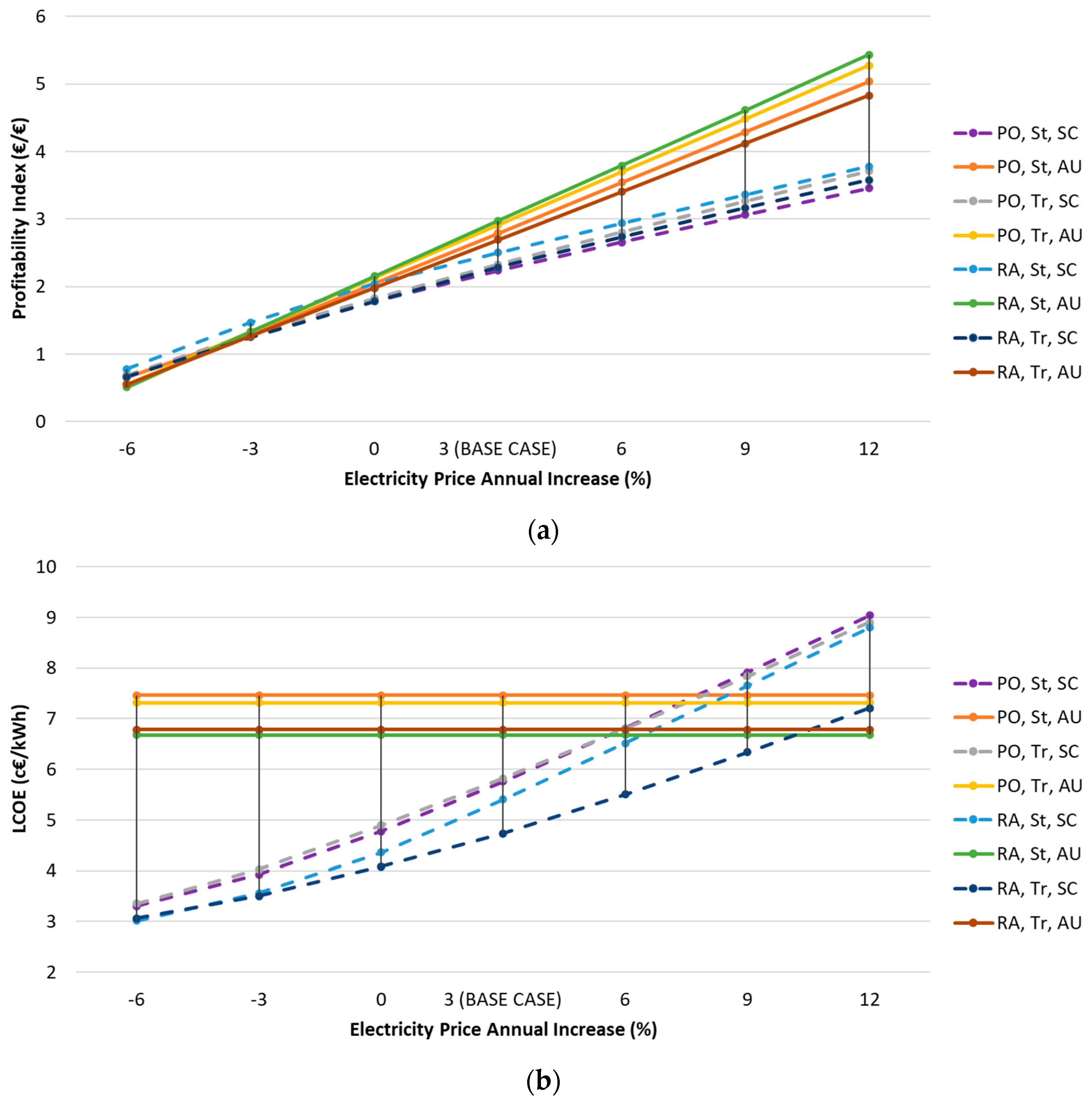
5.1. Annual Variation of Electricity Costs (PC and EC)

As mentioned in Section 3.2, Power Cost (PC) and Energy Cost (EC), which constitute the electricity costs, have been assumed to increase by 3% annually. Figure 6 presents the values of the PI (a), the LCOE (b) and the LCOE savings compared to the Only Grid Powered system (c), obtained for an annual variation of electricity costs between −6% and +12%. Note that IRR and PBP values are not presented, although they are also sensitive to this input, because with the PI it is easier to visually distinguish when the economic investment stops being profitable (PI < 1). Roughly, this would occur if electricity prices decreased by more than −3% annually, which is a rather unlikely scenario in the present energy landscape.

In terms of the PI, AU solutions (represented with the continuous lines) are more sensitive than the SC ones (represented with discontinuous lines), because the savings term S_n,AU varies more than S_n,SC -see Equations (3) and (4) -. On the other hand, the LCOE_AU does not vary, while the LCOE_SC increases exponentially with the electricity costs. In fact, the LCOE_AU could be less than the LCOE_SC for an annual increase of the electricity cost of more than 6%. As for the LCOE savings, they follow logarithmic functions for all the cases, but with a bigger coefficient for the AU solutions. Even if the electricity costs decreased by 3% annually, PV-HP systems would still be more economic than Only Grid-Powered ones.

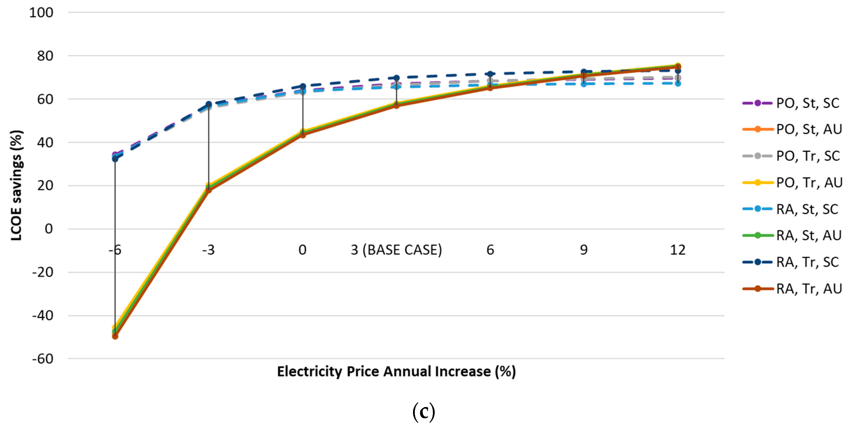
5.2. Interest Rate (i)

The profitability of the economic investment for installing PV-HP systems is very sensitive to the national interest rate. Even though IRR and PBP values do not change, the investment would only be profitable while i < IRR. Furthermore, the PI, the LCOE and the LCOE savings do experience significant variations with this input, as shown in Figure 7. The PI decreases when the i increases, according to a quadratic function. However, the i would have to increase nearly up to 10% for the investment not to be profitable, and not even for all the cases in this study. In developed countries like Spain, it is very unlikely that the interest rate would increase from 0.8% (the current value) to 10%. Finally, it can be observed that the LCOE increases exponentially with the i, while the LCOE savings also decrease exponentially. AU solutions (continuous lines) are more sensitive than SC solutions (discontinuous lines) because of their higher CFs, that experience bigger variations with the i when discounted to their present value.

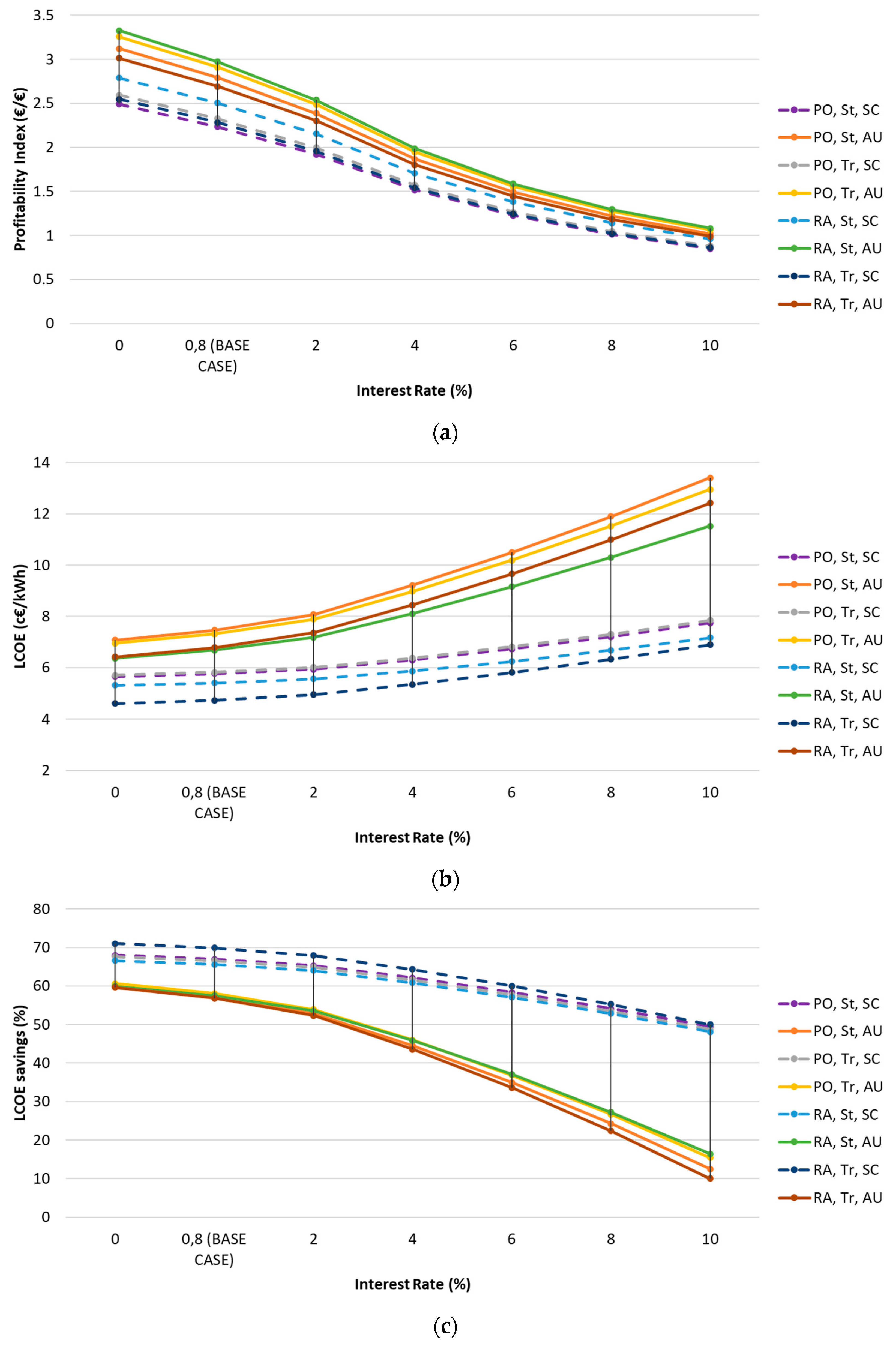
5.3. PV Surplus and Diesel Costs (SuC and DFC)

The economic profitability of PV-HP systems is not very sensitive to the variation of the SuC -in the case of SC solutions- or the DFC -in the case of AU solutions-, because they have little weight in comparison to the savings in terms of electricity costs. The LCOE and LCOE savings, on the other hand, experience significant variations as shown in Figure 8. For AU solutions, the LCOE increases linearly with the DFC and the LCOE savings decrease also linearly; for the SC solutions, the LCOE decreases logarithmically with the SuC and the LCOE savings increase also logarithmically. If both DFC and SuC decreased by −60%, the LCOE_AU would be bigger than the LCOE_SC. Although the DFC is not likely to decrease in the future, the SuC is susceptible to even bigger variations as the energy policies and markets evolve.

Note that Figure 8 can be used for analyzing scenarios where the PV surplus and the diesel costs did not experience the same variation, as each variable affect only a set of curves (SC or AU). For example, let us assume that the SuC decreased by −40% and the DFC increased by 20%. For the poultry farm with a static structure, we would need to compare the purple point corresponding to −40% (for an SC solution) and the orange point corresponding to 20% (for the AU solution).

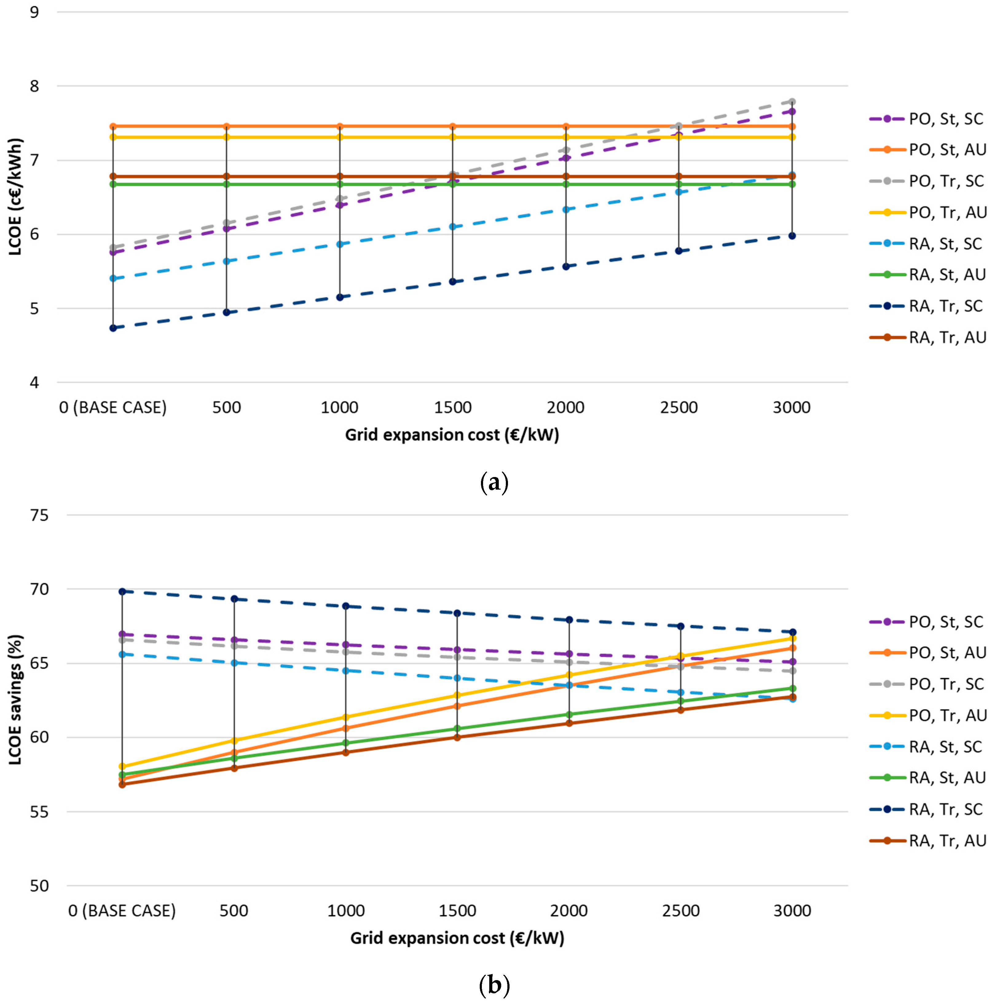
5.4. Grid Expansion Costs (GEC)

The previous analysis has been made under the assumption that there is a grid connection point available. Nevertheless, it is not uncommon that new farms are far from urban areas and isolated from any grid infrastructure. In that case, both Only Grid-powered and SC solutions would require an extra Initial Investment Cost to extend the grid, which would favor the AU solution economically. In order to explore this scenario, a sensitivity analysis to the grid expansion costs (GEC) has been carried out. Figure 9 presents the LCOE (a) and LCOE savings (b) obtained for a GEC in the 0–3000 €/kW range. The LCOE_SC increases linearly with the GEC; it could be bigger than the LCOE_AU if the GEC was higher than 2500 €/kW. As for the LCOE savings, they increase linearly for the AU solutions and decrease linearly for the SC solutions. If the GEC increased, the savings in the installation costs for an AU solution compared to an Only Grid-Powered system would be bigger. However, the saving for installing a SC solution (that needs a grid connection point) would be smaller. For example, if the GEC increased up to 3000 €/kW, the LCOE savings in a poultry farm with a tracking structure would be 3% points higher for an AU solution (yellow line, LCOE savings of 67%) than for a SC solution (grey line, LCOE savings of 64%).

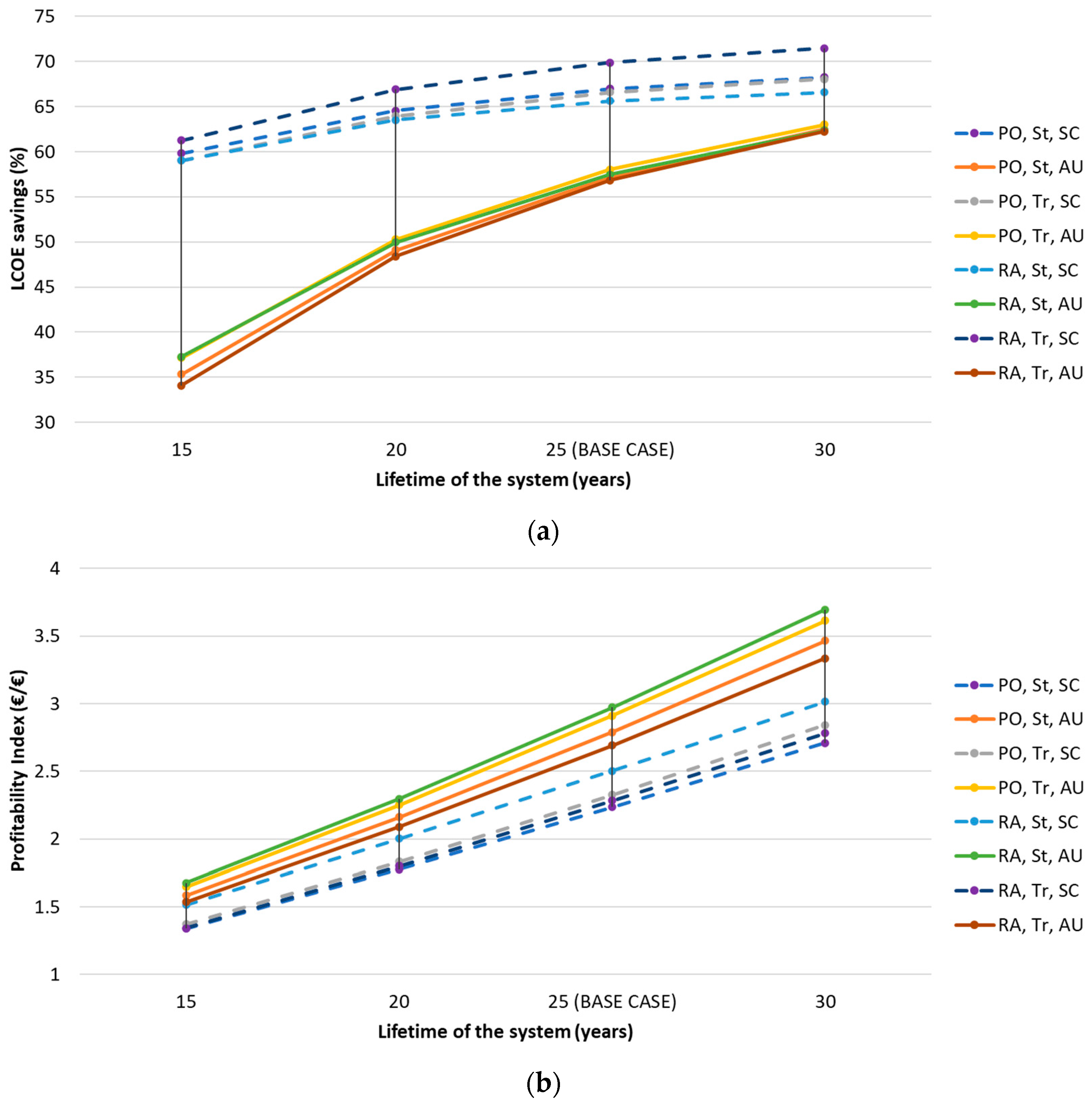
5.5. Lifetime of the System

This analysis has been made under the assumption that the system has a lifetime of 25 years. However, this lifetime could vary, especially for the PV generator if it suffered different degradation rates than the one assumed in this work (0.8% annually) [39]. Figure 10 presents the LCOE savings and the PI (b) obtained for a lifetime in the 15–30 years range. The LCOE savings increase logarithmically with the lifetime of the system, and the sensitivity is bigger for the AU solution. The PI increases exponentially and the sensitivity is also bigger for the AU solution. However, note that even for a lifetime of 15 years, less than the guarantees of PV modules (typically 25 years), the PV-HP implementation would still be profitable and LCOE savings would be more than 30%.

6. Conclusions

A recent work by the IES-UPM has developed a control algorithm for stand-alone PV-HP systems that permits up to 75% of the PV power fluctuations caused by passing clouds to be resisted [5] (hence eliminating the need for electric storage). This solution powers the compressor of the HP unit directly with a PV generator through a programmable frequency converter, mitigating solar power fluctuations by means of a PID control. This paper presents an economic assessment and comparison of this innovative autonomous (AU) solution for PV-HP systems for space heating and cooling (with water tanks as the thermal storage system and a diesel generator as back-up during winter) with a grid-connected configuration for PV self-consumption (SC). The AU system would operate with the control algorithm developed by the IES-UPM. These systems have been dimensioned for two livestock farms (a poultry farm and a bigger rabbit farm), considering the possibility of using static or tracking PV structures. This economic assessment has been carried out in terms of the profitability of the investment required to install a PV-HP system (given by the PI, the IRR and the PBP) and in terms of the LCOE, both in comparison to a traditional Only Grid Powered HP system. Finally, the robustness of the economic profitability of PV-HP systems has been tested by means of a sensitivity analysis. The main conclusions drawn from this analysis are the following:

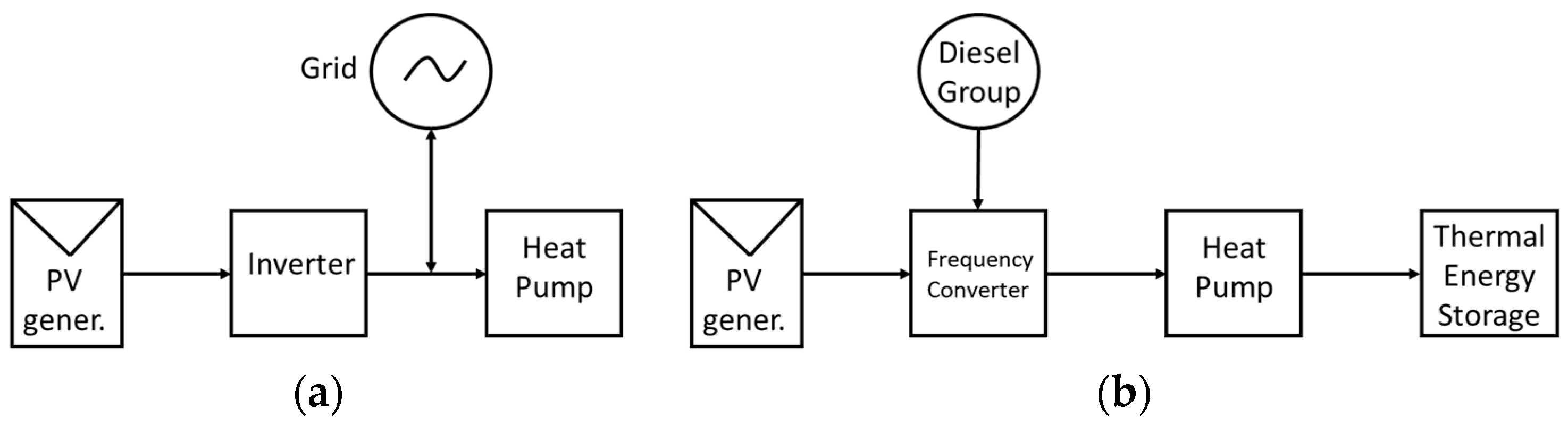
• SC solutions achieve bigger PV energy yields than AU solutions, because the PV surplus can be sold to the grid even when there is no consumption. Tracking structures obtain higher PV productions than static ones, hence requiring smaller PV systems for covering a certain demand.
• The PI values obtained are all positive and in the 2.23–2.97 €/€ range, all bigger than 1. AU solutions offer higher PIs than SC solutions (because they imply big savings in electricity costs).
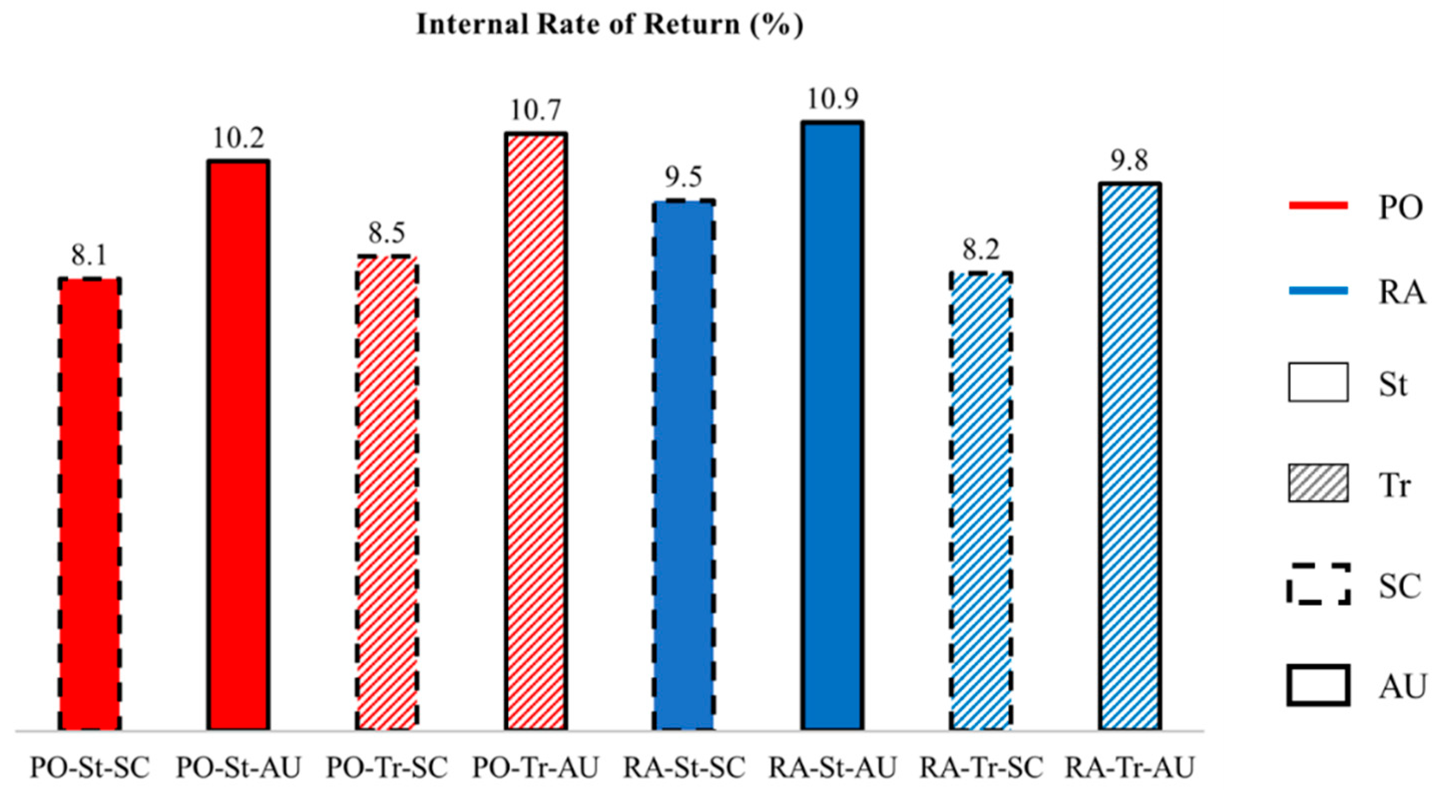
• The IRR values are in the 8.1–10.9% range, all higher than the interest rate (0.8%). AU solutions offer better profitability in term of IRR than SC solutions.
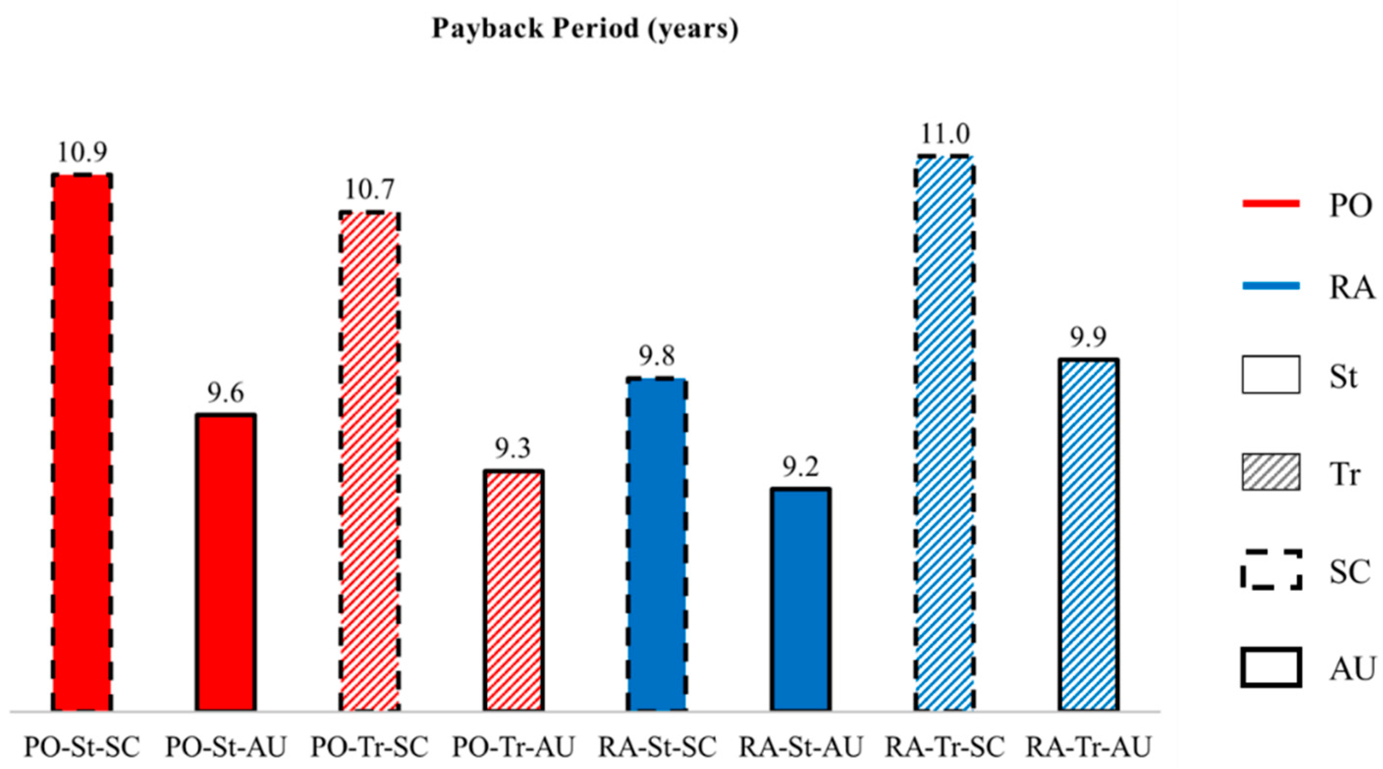
• The PBP values are in the 9.2–11 years range, all less than half the lifetime of the PV system (25 years). The bigger the IRR, the lower the PBP, so AU solutions permit to recover the economic investment sooner than the SC solutions.
• The LCOE values are in the 4.74–7.46 c€/kWh range, representing LCOE savings compared to the Only Grid-Powered system between 57% and 70%. Lower LCOEs (or higher LCOE savings) correspond to the SC solutions because of their higher energy yields.
• The PI, IRR and PBP express the economic profitability of a project and are the relevant selection criteria for an investor. The most significant factor for determining which solution is better are the economic savings in the electricity bill. The LCOE, on the other hand, expresses the energetic profitability of a project, helping to determine which option generates the maximum energy at the minimum cost. The most relevant factor in this case is the annual electricity production.
• The results are significantly sensitive to: the annual variation of electricity prices (the installation of a PV-HP system would be profitable unless these prices decreased by more than −3% annually, which is unlikely), the interest rate (PV-HP systems would be profitable unless it was more than 10%), the PV surplus cost -in the case of SC solutions- or the diesel cost -in the case of the AU solutions- (if both decreased by more than −60%, LCOE_AU could be lower than LCOE_SC), the grid expansion cost (if it was more than 2500 €/kW, LCOE_AU could be lower than LCOE_SC) and the lifetime of the system (although even for a lifetime of 15 years, PV-HP systems would still be profitable and generate LCOE savings of more than 30%).

In general terms, the installation of PV-HP systems instead of Only Grid-Powered HP systems for industrial space heating and cooling is already very profitable in economic and energetic terms. This profitability would only be endangered under certain circumstances that are not likely to occur in the present energy and financial landscape. Despite their higher LCOEs, AU solutions offer a better economic profitability than SC ones, because they permit bigger savings in terms of electricity costs, not only in the term of energy but also in the term of power.

References

- Lorenzo, C.; Narvarte, L. Performance indicators of photovoltaic heat-pumps. Heliyon 2019, 5, e02691. [Google Scholar] [CrossRef] [PubMed]
- European Heat Pump Association. European Heat Pump Online Assoaciation Stats Tool. Available online: http://www.stats.ehpa.org/hp_sales/story_sales (accessed on 6 April 2020).
- European Heat Pump Association. The European Heat Pump Market and Statistics Report 2019—Executive Summary. 2019. Available online: https://www.ehpa.org/fileadmin/red/07._Market_Data/2019/2019_Executive_Summary.pdf (accessed on 2 June 2020).
- Photovoltaics Report; Fraunhofer Institute for Solar Energy Systems: Freiburg, Germany, 2019.
- Lorenzo, C.; Narvarte, L.; Almeida, R.H.; Cristóbal, A.B. Technical evaluation of a stand-alone photovoltaic heat pump system without batteries for cooling applications. Sol. Energy 2020, 206, 92–105. [Google Scholar] [CrossRef]
- Aguilar, F.J.; Aledo, S.; Quiles, P.V. Experimental analysis of an air conditioner powered by photovoltaic energy and supported by the grid. Appl. Therm. Eng. 2017, 123, 486–497. [Google Scholar] [CrossRef]
- Romaní, J.; Belusko, M.; Alemu, A.; Cabeza, L.F.; de Gracia, A.; Bruno, F. Control concepts of a radiant wall working as thermal energy storage for peak load shifting of a heat pump coupled to a PV array. Renew. Energy 2018, 118, 489–501. [Google Scholar] [CrossRef]
- Opoku, R.; Mensah-Darkwa, K.; Muntaka, A.S. Techno-economic analysis of a hybrid solar PV-grid powered air-conditioner for daytime office use in hot humid climates–A case study in Kumasi city, Ghana. Sol. Energy 2018, 165, 65–74. [Google Scholar] [CrossRef]
- Aguilar, F.; Crespí-Llorens, D.; Quiles, P.V. Techno-economic analysis of an air conditioning heat pump powered by photovoltaic panels and the grid. Sol. Energy 2019, 180, 169–179. [Google Scholar] [CrossRef]
- Roselli, C.; Sasso, M.; Tariello, F. Dynamic Simulation of a Solar Electric Driven Heat Pump for an Office Building Located in Southern Italy. Int. J. Heat Technol. 2016, 34, S496–S504. [Google Scholar] [CrossRef]
- Gantenbein, L.O.P.; Notter, D.; Snegirjovs, A. Combined PV solar compression cooling and free cooling system. In Proceedings of the 32nd European Photovoltaic Solar Energy Conference and Exhibition, Munich, Germany, 20–24 June 2016. [Google Scholar]
- Li, Y.; Zhao, B.Y.; Zhao, Z.G.; Taylor, R.A.; Wang, R.Z. Performance study of a grid-connected photovoltaic powered central air conditioner in the South China climate. Renew. Energy 2018, 126, 1113–1125. [Google Scholar] [CrossRef]
- Rudischer, R.; Waschull, J.; Hernschier, W.; Friebe, C. Available solar cooling applications for different purposes. In Proceedings of the 1st International Conference of Solar Air-Conditioning, Bad Staffelstein, Germany, 6–7 October 2005. [Google Scholar]
- Daut, I.; Adzrie, M.; Irwanto, M.; Ibrahim, P.; Fitra, M. Solar Powered Air Conditioning System. Energy Procedia 2013, 36, 444–453. [Google Scholar] [CrossRef][Green Version]
- SISIFO Simulation Tool. Available online: https://www.sisifo.info/es/default (accessed on 3 June 2020).
- International Energy Agency (IEA). Average CO2 Emissions Intensity of Hourly Electricity Supply in the European Union, 2018 and 2040 by Scenario and Average Electricity Demand in 2018. Available online: https://www.iea.org/data-and-statistics/charts/average-co2-emissions-intensity-of-hourly-electricity-supply-in-the-european-union-2018-and-2040-by-scenario-and-average-electricity-demand-in-2018 (accessed on 22 July 2020).
- Product Catalogue 2018–2019. Available online: https://www.keyter.com/downloads/ (accessed on 5 June 2020).
- Hauer, A. Thermal energy storage. Energy Technology System Analysis Programme (ETSAP) and International Renewable Energy Agency (IRENA). Technology Policy Brief E17. January 2013. Available online: https://iea-etsap.org/E-TechDS/HIGHLIGHTS%20PDF/E17IR%20ThEnergy%20Stor_AH_Jan2013_final_GSOK%201.pdf (accessed on 2 June 2020).
- PVGIS Database. Available online: https://ec.europa.eu/jrc/en/pvgis (accessed on 3 June 2020).
- Erbs, D.G.; Klein, S.A.; Duffie, J.A. Estimation of the diffuse radiation fraction for hourly, daily and monthly-average global radiation. Sol. Energy 1982, 28, 293–302. [Google Scholar] [CrossRef]
- Collares-Pereira, M.; Rabl, A. The average distribution of solar radiation-correlations between diffuse and hemispherical and between daily and hourly insolation values. Sol. Energy 1979, 22, 155–164. [Google Scholar] [CrossRef]
- Perez, R.; Seals, R.; Ineichen, P.; Stewart, R.; Menicucci, D. A new simplified version of the perez diffuse irradiance model for tilted surfaces. Sol. Energy 1987, 39, 221–231. [Google Scholar] [CrossRef]
- Martínez-Moreno, F.; Muñoz, J.; Lorenzo, E. Experimental model to estimate shading losses on PV arrays. Sol. Energy Mater. Sol. Cells 2010, 94, 2298–2303. [Google Scholar] [CrossRef]
- Crundwell, F.K. Finance for Engineers, Evaluation and Funding of Capital Projects; Springer: London, UK, 2008. [Google Scholar]
- Vartiainen, E.; Masson, G. PV LCOE in Europe 2015–2050. In Proceedings of the 31st European Photovoltaic Solar Energy Conference and Exhibition, Hamburg, Germany, 14–18 September 2015. [Google Scholar]
- Lorenzo, C.; Almeida, R.H.; Martínez-Núñez, M.; Narvarte, L.; Carrasco, L.M. Economic assessment of large power photovoltaic irrigation systems in the ECOWAS region. Energy 2018, 155, 992–1003. [Google Scholar] [CrossRef]
- Jefatura de Estado, D.L. M-1/1958-ISSN: 0212-033X, Ley 27/2014, del 27 de noviembre, del Impuesto sobre Sociedades. 2014. Available online: https://www.boe.es/boe/dias/2015/03/13/pdfs/BOE-A-2015-2668.pdf (accessed on 4 June 2020).
- Trending Economics, Spain Indicators. Available online: https://tradingeconomics.com/spain/indicators (accessed on 7 April 2020).
- Ministerio de Economía. Real decreto 1164/2001, de 26 de octubre, por el que se establecen tarifas de acceso a las redes de transporte y distribución de energía eléctrica. 2001. Available online: https://www.boe.es/eli/es/rd/2001/10/26/1164 (accessed on 4 June 2020).
- Operador del Mercado Ibérico de Energía (OMIE). Componentes Precio Final Medio de la Demanda Nacional. Available online: https://www.omie.es/es/market-results/interannual/average-final-prices/components-spanish-demand?scope=interannual (accessed on 3 June 2020).
- Agencia Tributaria. Impuestos Especiales, Capítulo 6 (Impuesto Especial Sobre la Electricidad). 2015. Available online: https://www.agenciatributaria.es/static_files/AEAT/Aduanas/Contenidos_Privados/Impuestos_especiales/Estudio_relativo_2009/06elec.pdf (accessed on 4 June 2020).
- Expansion Datosmacro. Precios de los Derivados del Petróleo en España. Available online: https://datosmacro.expansion.com/energia/precios-gasolina-diesel-calefaccion/espana?anio=2019 (accessed on 3 June 2020).
- European Central Bank. Inflation Rate. Available online: http://sdw.ecb.europa.eu/ (accessed on 3 June 2020).
- Carrêlo, I.B.; Almeida, R.H.; Narvarte, L.; Martinez-Moreno, F.; Carrasco, L.M. Comparative analysis of the economic feasibility of five large-power photovoltaic irrigation systems in the Mediterranean region. Renew. Energy 2020, 145, 2671–2682. [Google Scholar] [CrossRef]
- Range, A.d.S.; Santos, J.C.d.S.; Savoia, J.R.F. Modified Profitability Index and Internal Rate of Return. J. Int. Bus. Econ. 2016, 4. [Google Scholar] [CrossRef]
- U.S. Energy Information Administration. Levelized Cost and Levelized Avoided Cost of New Generation Resources in the Annual Energy Outlook 2020; February 2020. Available online: https://www.eia.gov/aeo (accessed on 5 June 2020).
- Coady, D.; Parry, I.; Sears, L.; Shang, B. How large are global energy subsidies? World Dev. 2017, 91, 11–27. [Google Scholar] [CrossRef]
- Todde, G.; Murgia, L.; Carrelo, I.; Hogan, R.; Pazzona, A.; Ledda, L.; Narvarte, L. Embodied Energy and Environmental Impact of Large-Power Stand-Alone Photovoltaic Irrigation Systems. Energies 2018, 11, 2110. [Google Scholar] [CrossRef]
- Jordan, D.C.; Silverman, T.J.; Sekulic, B.; Kurtz, S.R. PV degradation curves: Non-linearities and failure modes. Prog. Photovolt. Res. Appl. 2017, 25, 583–591. [Google Scholar] [CrossRef]