Generalized Fault-Location Scheme for All-Parallel AT Electric Railway System

Abstract

The existing fault location methods for all-parallel autotransformer railway systems (AARS) have limitations because they are generally designed for several given feeding conditions. In alternate feeding conditions, the existing fault location methods do not work well and may have large errors. To solve this problem, we have proposed a generalized fault location scheme for AARS in this paper. After analyzing the fault characteristics of AARS, we classified the feeding conditions of the faulted section of AARS into three types and introduced the corresponding fault location methods. In order to identify the faulted section and its feeding condition, we first formed a switch state matrix based on the adjacency matrix and mapped the fault current distribution into a current state matrix, then we unified the two matrices into a fault state matrix to reflect the fault state of the AARS. Finally, a generalized fault location scheme was proposed based on a fault state matrix. The proposed scheme effectively eliminates the negative influence of feeding conditions on the fault location, and it can identify the fault type and locate faults in different feeding conditions. Several simulation cases verified the effectiveness of the proposed scheme.

1. Introduction

Short-circuit faults occur very frequently and are often inevitable in all-parallel autotransformer (AT) railway systems (AARS). Therefore, locating the fault is very important for reducing outage time and loss of revenue. The current fault location methods are mainly designed for normal feeding conditions of AARS and are highly accurate in engineering applications. However, due to user operation or repairing equipment out of service, circuit breakers can open and the railway system is no longer in a normal feeding condition, which means that the existing fault location methods no longer work well.

In the past, various fault location algorithms for railway systems have been proposed whereby impedance-based methods and current-ratio-based methods are widely used [1]. Impedance methods are very attractive because of their simplicity and low implementation cost [2,3]. In practice, fault resistance normally exists at a fault point. To avoid the influence of fault resistance on the fault location, measured reactance is used to locate a fault; hence impedance methods are also called reactance methods [4,5,6]. Reactance methods are widely used for a single-line track return railway system, since the short-circuit reactance value of faulted catenary wire increases linearly in proportion to the fault distance. Recently, an improved reactance method was proposed to eliminate the influence of mutual reactance on the fault location for a double-line railway system [7]. However, reactance methods are not suitable for catenary-rail (C-R) faults and feeder-rail (F-R) faults in AT railway systems because the presence of AT makes short-circuit impedance non-linear with the fault distance. The most used fault location methods in AT railway systems are the neutral current ratio method [8] and the up and down current ratio method [9]. To compensate for the neutral currents circulating in adjacent autotransformers, a revision algorithm with the neutral current ratio method has been proposed [10]. Recently, methods derived from the neutral current ratio were also proposed in [11,12]. Many researchers have proposed to use of traveling wave methods for the fault location scheme of AC electric railway systems [13,14,15]. However, traveling wave method have been well proven in high-voltage transmission systems but not in railway systems.

In practice, the neutral current ratio method and up and down current ratio method are widely used for fault location in AARS, because of their high accuracy and they are not influenced by fault resistance. However, these methods are based on the fault current relationship of a specific railway feeding scheme; therefore, they can be only adopted in the relevant feeding conditions. The neutral current ratio method only works in the feeding condition with ATs in service. The up and down current ratio method is only suitable for normal feeding condition in which all circuit breakers are closed, i.e., all up and down lines are in parallel connection at the substation (SS) and the AT post (ATP), and they do not work when some circuit breakers are open.

From the above discussion we know that the existing fault location methods are designed only for certain feeding conditions. When some circuit breakers are open to meet the needs of the electric railway system, the feeding condition is changed. Because the fault current distribution changes with the feeding condition, the fault location method must change correspondingly. If we consider the states of all circuit breakers for a railway system with 2n circuit breakers, theoretically there are $3\times 2^{2(n-1)}$ feeding conditions because the up and down line circuit breakers at the SS cannot both be open. For example, for a AT railway system with eight circuit breakers, there are 192 feeding conditions. Therefore, it is difficult to use exhaustive methods to identify each of feeding conditions and design a corresponding fault location method.

To solve this problem, we proposed a generalized fault location method for AARS that considers the relationship between the fault current distribution and feeding condition according to the characteristics of the fault state matrix. Our main contributions can be summarized as follows.

• To simplify the fault location scheme to match different feeding conditions, we classified the feeding conditions of faulted sections into three types and introduced the corresponding fault location methods, thus we improved the up and down current ratio method, neutral current ratio method and reactance method for long-section feeding conditions.
• To identify the faulted section and its feeding condition, we first formed a switch state matrix based on the adjacency matrix and mapped the fault current distribution into a current state matrix, then we unified the two matrices into a fault state matrix to reflect the fault state of AARS.
• To achieve accurate fault location in each of the feeding conditions, we proposed a generalized fault location scheme combining the fault location method and fault identification.

The remainder of this paper is organized as follows. Section 2 introduces the fault characteristics of AARS. Section 3 classifies the feeding conditions and introduces the corresponding improved fault location methods. Section 4 proposes a generalized fault location scheme for AARS. In Section 5, the results of the simulation tests are discussed. The conclusions are presented in Section 6.

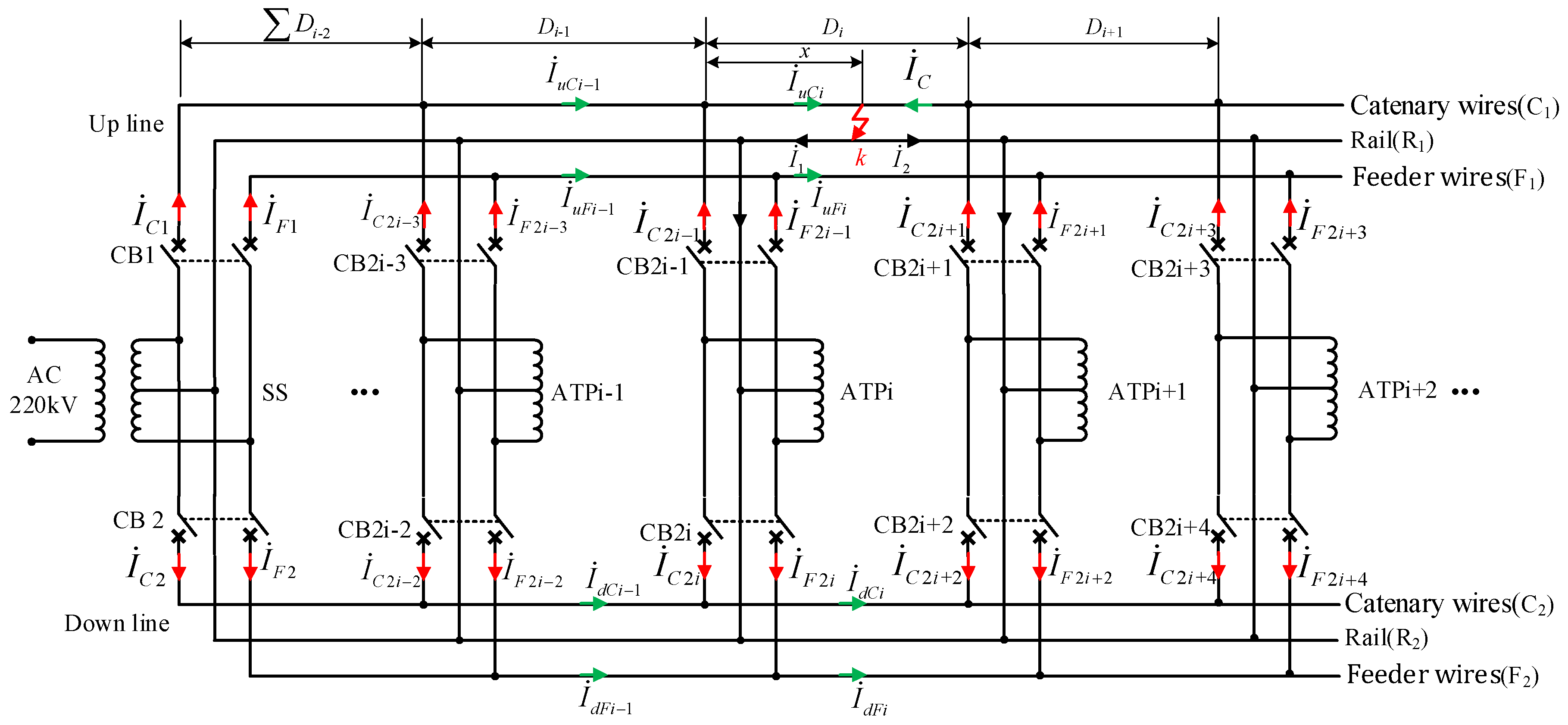
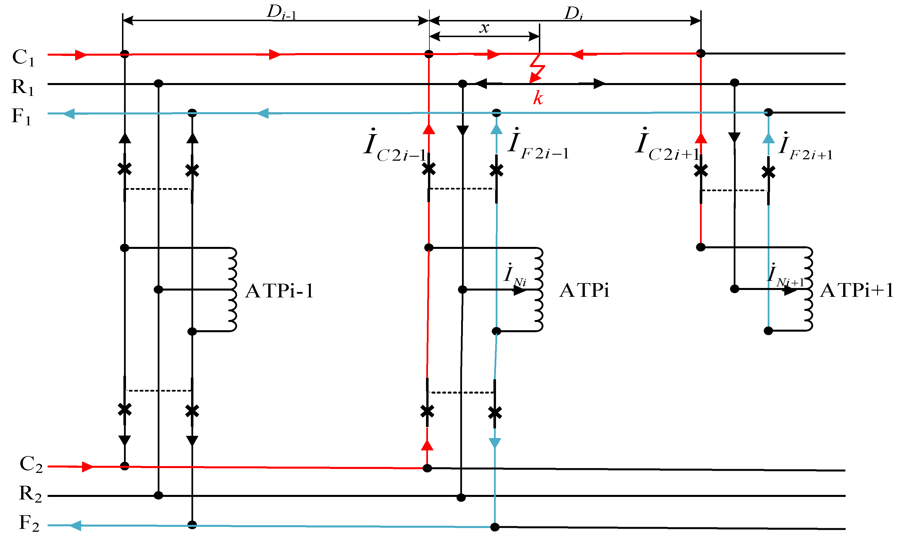
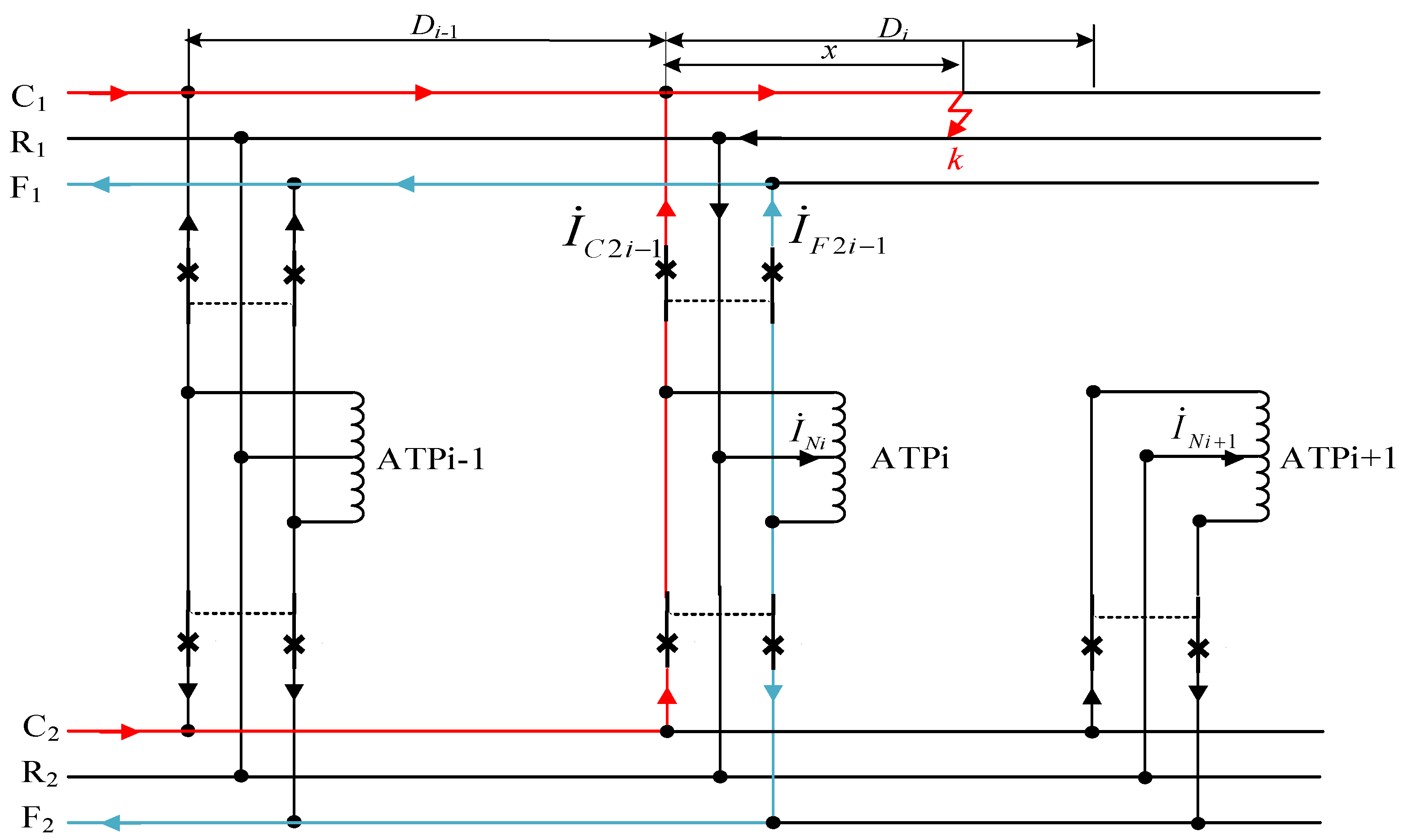
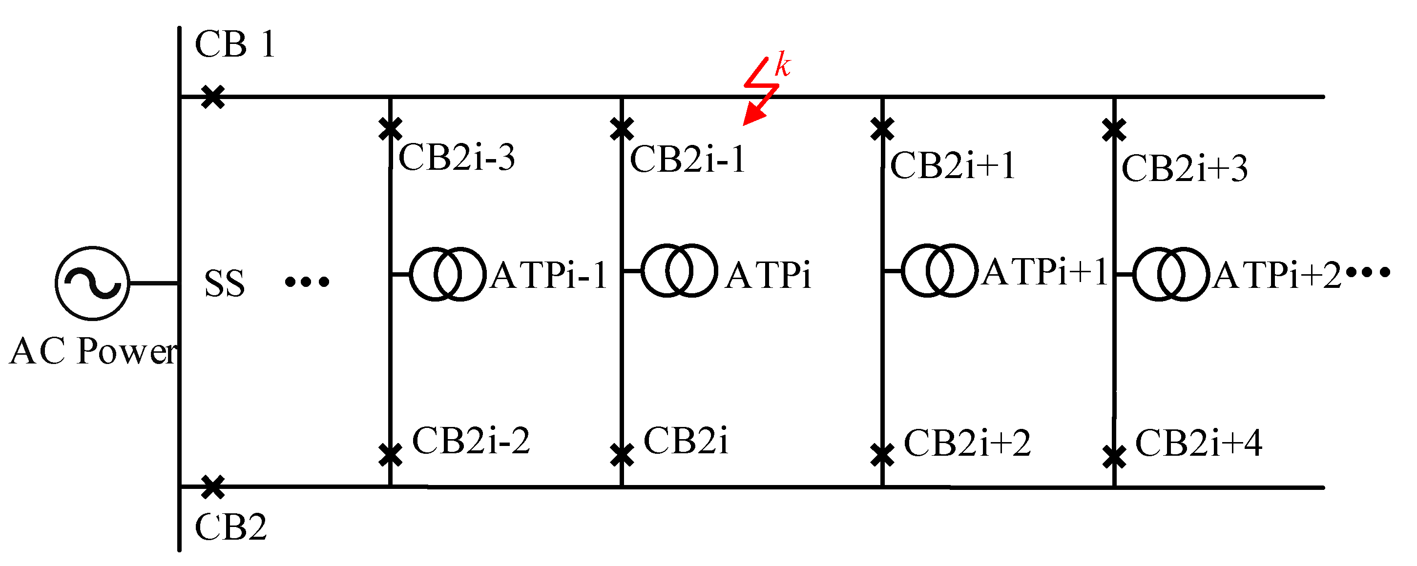
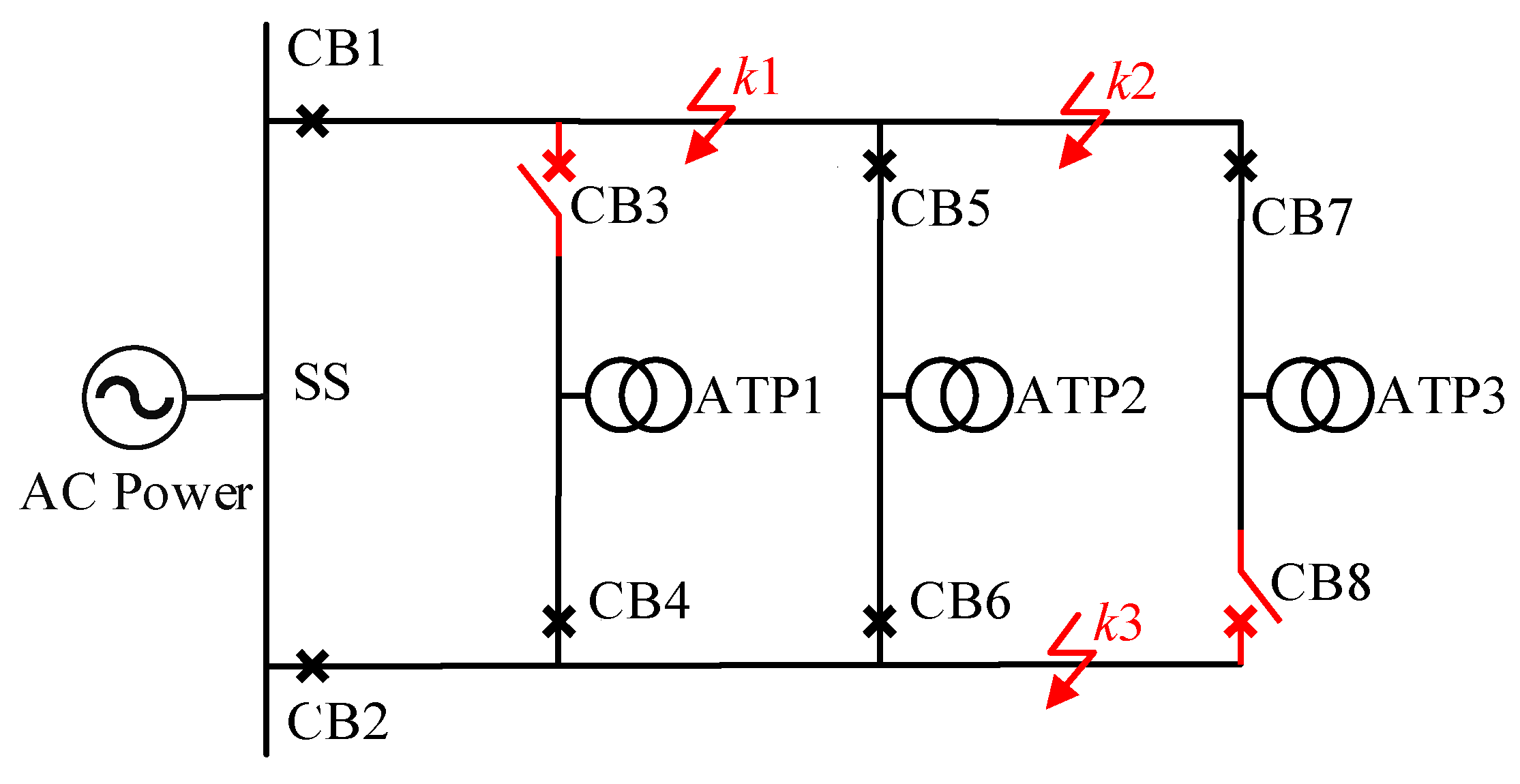
2. Fault Characteristics of AARS

The AARS is generally used to cope with peak power requirements and improve inductive interference in high-speed railways; and it provides a 25–0–25 kV AC supply consisting of catenary (C) wires and feeder (F) wires [16,17]. Moreover, ATs are connected to the busbars in the AT post where up and down wires are in parallel to ensure a stable voltage. The system generally has two or three AT sections in normal feeding conditions and four to six AT sections in over-zone feeding conditions. In order to show the generality of our method, an AARS with 2n circuit breakers is shown in Figure 1.

In Figure 1, SS denotes the substation and ATPi (i = 2…n) denotes AT post. $D_i$ (i = 1…n − 1) denotes the length of the AT section i between ATPi and ATPi+1, CBi (i = 1…2n) denotes two-pole line circuit breaker, and the system forms many feeding conditions with CB1-CB2n open or close. ${\dot{I}}_{Ci}$ (i = 1…2n) denotes the catenary current of CBi and ${\dot{I}}_{Fi}$ (i = 1…2n) denotes the feeder current of CBi. We used the C-R fault at point k as an example to analyze the characteristics of fault current, as it is similar to F-R or C-F faults. The fault characteristics are as follows.

(1) Because the AT turns ratio is 1, based on Kirchhoff’s Current Law (KCL) we know that the fault currents of each AT section before the fault point are equal. As shown in Figure 1, we can use the following equation:

$${\dot{I}}_{u1}+{\dot{I}}_{d1}=\dots ={\dot{I}}_{ui-1}+{\dot{I}}_{di-1}={\dot{I}}_{ui}+{\dot{I}}_{di}$$

(1)

where ${\dot{I}}_{ui}$, ${\dot{I}}_{di}$ denote the fault currents, respectively flowing through section i of the up and down line, ${\dot{I}}_{ui}={\dot{I}}_{uCi}-{\dot{I}}_{uFi}$, ${\dot{I}}_{di}={\dot{I}}_{dCi}-{\dot{I}}_{dFi}$.

(2) The first parallel connections before and after the fault point bypass the other ATP parallel lines; therefore, the parallel currents flowing through non-first parallel lines are very small, and the first parallel current after the fault point are close to the fault current flowing through the healthy line of the faulted section. As shown in Figure 1, we can obtain that by

$${\dot{I}}_{di}={\displaystyle \sum _{j=i+1}^n{\dot{I}}_{Pj}}\approx {\dot{I}}_{Pi+1}$$

(2)

where ${\dot{I}}_{Pi}$ (i = 2…n) denotes the parallel current flowing through ATPi, ${\dot{I}}_{C2i-1}-{\dot{I}}_{F2i-1}={\dot{I}}_{Pi}={\dot{I}}_{F2i}-{\dot{I}}_{C2i}$.

(3) Because of the symmetry of AARS, the up and down currents of healthy wires in each parallel ATP have the same magnitude and direction (both from the ATP to the line, or both from the line to the ATP). For a C-R fault as shown in Figure 1, we can obtain that by

$${\dot{I}}_{F2i-1}={\dot{I}}_{F2i}(i=1\dots n)$$

(3)

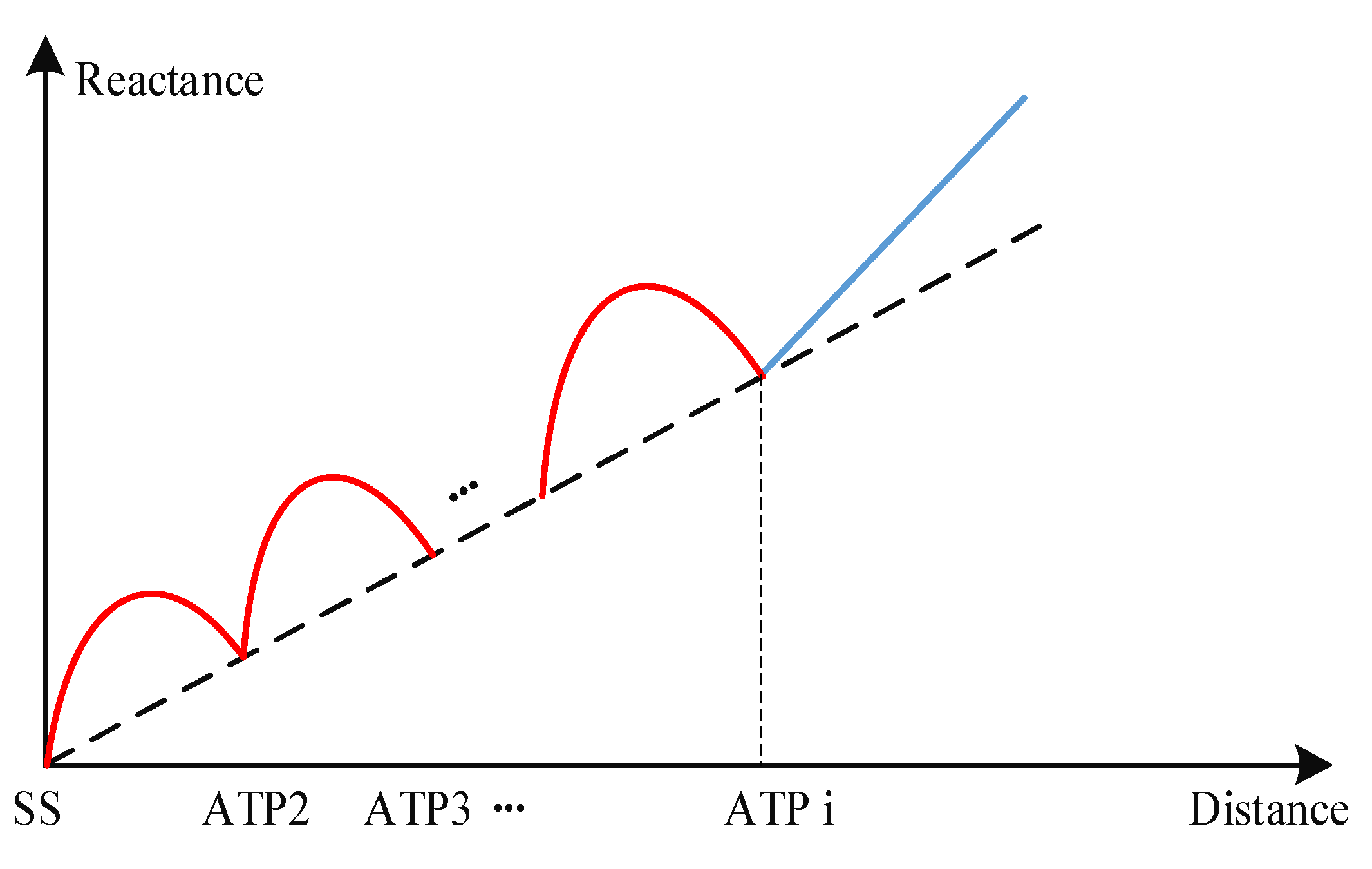
3. Classification of Feeding Conditions of the Faulted Section and Fault Location Methods

The change in feeding conditions will affect the topology of the railway system and thus the current distribution; therefore, different fault location methods need to be adopted. Considering the state of all circuit breakers for a railway system with 2n circuit breakers, there are $3\times 2^{2(n-1)}$ feeding conditions. It is difficult to identify each of feeding conditions and apply corresponding fault location methods. However, if we focus on the faulted section we can observe that the fault current distribution of the faulted section is only related to the feeding condition of the faulted section but not to the other sections. Therefore, we can focus on the feeding conditions of the faulted section to find a fault location scheme so as not to exhaust each of the feeding conditions of the AARS. According to our analysis, the feeding conditions of the faulted section can be divided into three types as follows.

(1) “Up-down parallel” (UDP) feeding condition: the up and down lines are connected through parallel lines on both ends of the faulted section. For example, if a fault occurs at point k with CB 2i-1 open as shown in Figure 1, the corresponding current distribution of the faulted long section between ATPi-1 and ATPi+1 is as shown in Figure 2. Meanwhile, C, F and R of the up and down lines are connected in parallel by the parallel lines of ATPi-1 and ATPi+1 to form three closed loops.

Therefore, we can obtain the Equation of C1-C2 loop (red lines) based on Kirchhoff’s Voltage Law (KVL) as follows

$$\begin{array}{l}x(\dot{I}-{\dot{I}}_C)Z_C-(D_{i-1}+D_i-x){\dot{I}}_C{Z}_C-x{\dot{I}}_1{Z}_{CR}+(D_{i-1}+D_i-x){\dot{I}}_2{Z}_{CR}-(D_{i-1}+D_i){\dot{I}}_F{Z}_{CF}\\ =(D_{i-1}+D_i)\left[-(\frac{{\dot{I}}_2-{\dot{I}}_0}{2}-{\dot{I}}_C)Z_C-{\dot{I}}_0{Z}_{CR}-(\frac{{\dot{I}}_2-{\dot{I}}_0}{2}-{\dot{I}}_F)Z_{CF}\right]+D_{i-1}\left[-\frac{1}{2}{\dot{I}}_{Ni}{Z}_C+{\dot{I}}_{Ni}{Z}_{CR}-\frac{1}{2}{\dot{I}}_{Ni}{Z}_{CF}\right]\end{array}$$

(4)

Similarly, the F1-F2 loop (blue lines) and R1-R2 loop (black lines) represent Equations (5) and (6), respectively, as follows

$$\begin{array}{l}x(\dot{I}-{\dot{I}}_C)Z_{CR}-(D_{i-1}+D_i-x){\dot{I}}_C{Z}_{CR}-x{\dot{I}}_1{Z}_R+(D_{i-1}+D_i-x){\dot{I}}_2{Z}_R-(D_{i-1}+D_i){\dot{I}}_F{Z}_{RF}\\ =(D_{i-1}+D_i)\left[-(\frac{{\dot{I}}_2-{\dot{I}}_0}{2}-{\dot{I}}_C)Z_{CR}-{\dot{I}}_0{Z}_R-(\frac{{\dot{I}}_2-{\dot{I}}_0}{2}-{\dot{I}}_F)Z_{RF}\right]+D_{i-1}\left[-\frac{1}{2}{\dot{I}}_{Ni}{Z}_{CR}+{\dot{I}}_{Ni}{Z}_R-\frac{1}{2}{\dot{I}}_{Ni}{Z}_{RF}\right]\end{array}$$

(5)

$$\begin{array}{l}x(\dot{I}-{\dot{I}}_C)Z_{CF}-(D_{i-1}+D_i-x){\dot{I}}_C{Z}_{CF}-x{\dot{I}}_1{Z}_{RF}+(D_{i-1}+D_i-x){\dot{I}}_2{Z}_{RF}-(D_{i-1}+D_i){\dot{I}}_F{Z}_F\\ =(D_{i-1}+D_i)\left[-(\frac{{\dot{I}}_2-{\dot{I}}_0}{2}-{\dot{I}}_C)Z_{CF}-{\dot{I}}_0{Z}_{RF}-(\frac{{\dot{I}}_2-{\dot{I}}_0}{2}-{\dot{I}}_F)Z_F\right]+D_{i-1}\left[-\frac{1}{2}{\dot{I}}_{Ni}{Z}_{CF}+{\dot{I}}_{Ni}{Z}_{RF}-\frac{1}{2}{\dot{I}}_{Ni}{Z}_F\right]\end{array}$$

(6)

where $Z_C,Z_F,Z_R$ denote the per-unit impedance of lines C, F and R, respectively; $Z_{CR},Z_{CF},Z_{RF}$ denote the per-unit mutual impedance between the lines C, F and R, respectively; and ${\dot{I}}_{Ni}$ denotes the neutral current of ATPi.

From Equations (4)–(6), we obtain the following

$$\{\begin{array}{c}{\dot{I}}_C=\frac{x}{2(D_{i-1}+D_i)}\dot{I}+\frac{{\dot{I}}_2-{\dot{I}}_0}{4}+\frac{D_{i-1}{\dot{I}}_{Ni}}{4(D_{i-1}+D_i)}\\ {\dot{I}}_F=\frac{{\dot{I}}_2-{\dot{I}}_0}{4}+\frac{D_{i-1}{\dot{I}}_{Ni}}{4(D_{i-1}+D_i)}\end{array}$$

(7)

The currents of the up and down section lines are as follows

$$\{\begin{array}{l}{\dot{I}}_{ui-1}=\dot{I}-{\dot{I}}_C+{\dot{I}}_F==\frac{2(D_{i-1}+D_i)-x}{2(D_{i-1}+D_i)}\dot{I}\\ {\dot{I}}_{di-1}={\dot{I}}_C-{\dot{I}}_F=\frac{x}{2(D_{i-1}+D_i)}\dot{I}\end{array}$$

(8)

Therefore, the fault distance x has a unique solution as follows

$$x=\left|\frac{{\dot{I}}_{di-1}}{{\dot{I}}_{ui-1}+{\dot{I}}_{di-1}}\right|\times 2(D_{i-1}+D_i)$$

(9)

By combining Equations (1) and (2), we obtain

$$x=\left|\frac{{\dot{I}}_{Pi+1}}{{\dot{I}}_{u1}+{\dot{I}}_{d1}}\right|\times 2(D_{i-1}+D_i)$$

(10)

When a C-F or F-R fault occurs in AARS, we can obtain the same fault location method as Equation (10). If the faulted section is in the UDP feeding condition, the above fault distance can be obtained regardless of the connection of the AT (such as ATPi in Figure 2). By extension, if a fault occurs in a long section between ATPa and ATPb in the UDP feeding condition, we can obtain a generalized up and down current ratio method as follows

$$x=\left|\frac{{\dot{I}}_{Pi+1}}{{\dot{I}}_{u1}+{\dot{I}}_{d1}}\right|\times 2(D_{i-1}+D_i)$$

(11)

(2) “Single-line AT” (SLAT) feeding condition: ATs are connected on both ends of the faulted section. For example, if a C-R or F-R fault occurs at point k in the section between ATPi and ATPi+1 with CB $2j(j=i+1\dots n)$ open, where the faulted section is in the SLAT feeding condition as shown in Figure 3.

We can use the neutral current ratio method [7] to locate the fault as follows

$$x=\left|\frac{{\dot{I}}_{Ni+1}}{{\dot{I}}_{Ni}+{\dot{I}}_{Ni+1}}\right|\times D_i=|\frac{{\dot{I}}_{C2i+1}+{\dot{I}}_{F2i+1}}{{\dot{I}}_{C2i-1}+{\dot{I}}_{F2i-1}+{\dot{I}}_{C2i+1}+{\dot{I}}_{F2i+1}}|\times D_i$$

(12)

By extension, when a C-R or F-R fault occurs in a long section in SLAT feeding conditions between ATPa and ATPb with CB $2j(j=a+1\dots n)$ and CB $2j-1(j=a+1\dots b-1)$ open, we can obtain a generalized neutral current ratio method as follows

$$x_2=|\frac{{\dot{I}}_{C2b-1}+{\dot{I}}_{F2b-1}}{{\dot{I}}_{C2a-1}+{\dot{I}}_{F2a-1}+{\dot{I}}_{C2b-1}+{\dot{I}}_{F2b-1}}|\times {\displaystyle \sum _{i=a}^{b-1}{D}_i}$$

(13)

Because neutral currents are very small for a C-F fault, we use the reactance method to locate the fault in SLAT feeding conditions.

(3) “Single-line track return” (SLTR) feeding condition: the circuit breakers after the fault point in the faulted line are all open. In this section, only running rails and earth are used to conduct return currents. For example, if a fault occurs at point k on the up line after ATPi with CB 2i-1 closed and CB $2j-1(j=i+1\dots n)$ open, where the faulted section is in SLTR feeding condition as shown in Figure 4. In this condition, the measured reactance at the SS is affected by the feeding condition of the sections before ATPi. In contrast, the measured reactance at ATPi can be used to locate the fault because the fault distance from the fault point to ATPi is linear with the measured reactance. Figure 5 illustrates the typical measured reactance with the fault distance.

Therefore, we can use the measured reactance at CB 2i-1 to locate the fault by using the reactance method [3] as follows

$$x_3=\frac{X_{2i-1}}{x_a}$$

(14)

where $X_{2i-1}$ denotes the measured reactance at CB 2i − 1, $x_a$ denotes the per-unit reactance for the C-R, F-R or C-F fault. The fault location method needs to identify the fault type and uses the corresponding per-unit reactance.

4. Generalized Fault Location Scheme

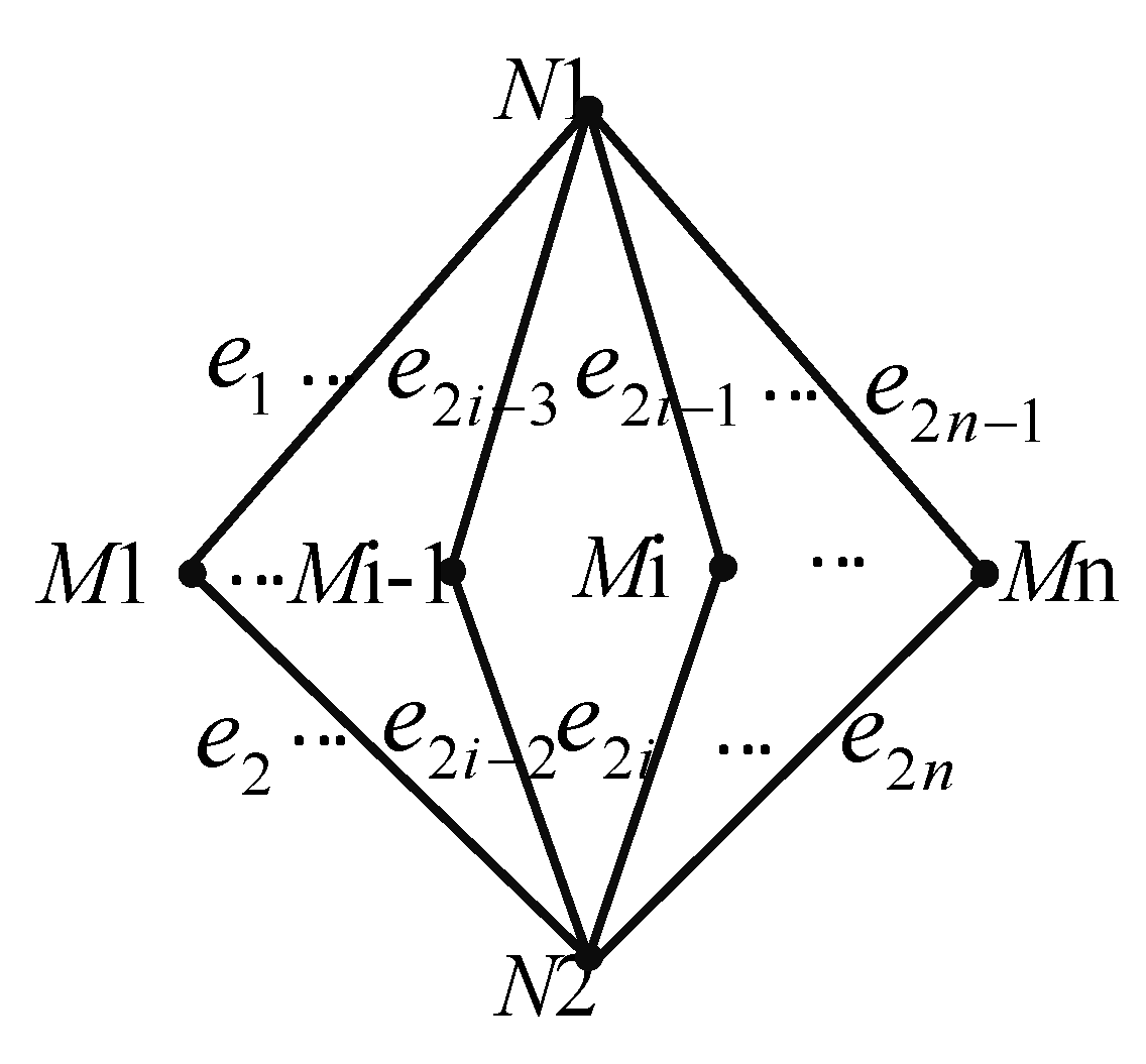
4.1. Fault State Matrix

From Section 3, we know that for fault location it is important to identify the faulted section and its feeding condition. Because the circuit breakers are two-pole, it is easier to use the sing-line diagram to identify the feeding condition as shown in Figure 6.

The feeding conditions of AARS are decided by the system topology, which is structured by circuit breakers; therefore, we used an adjacency matrix [18,19] to describe the topological structure and feeding conditions. In Figure 6, we regard the up and down lines as generalized nodes, ATPi as intermediate nodes, and circuit breakers as branches that reflect the connection of nodes; therefore, the connection diagram of AARS can be obtained as shown in Figure 7.

$M1,M2\dots Mn$, the intermediate nodes; $e_i=0/1(i=1,2\cdots 2n)$, branch.

The corresponding adjacency matrix is $A$ as follows

(15)

It can be seen from the above-mentioned matrix that the correlation of the nodes depend on the branches (i.e., the states of 2n circuit breakers) as shown by the red dotted box in Equation (15). To simplify the analysis, the branches are selected to form a new matrix $A_Q$ called the switch state matrix as follows

$$A_Q=\left[\begin{array}{lllll}{e}_1\hfill & e_3\hfill & e_5\hfill & \dots \hfill & e_{2n-1}\hfill \\ e_2\hfill & e_4\hfill & e_6\hfill & \dots \hfill & e_{2n}\hfill \end{array}\right]$$

(16)

Therefore, the characteristics of the topological structure of the above three types of feeding conditions can be summarized as follows

(1) UDP: there are at least two pathways between N1 and N2, and they are distributed on both ends of the faulted section. If a fault occurs at point k with CB 2i-1 open as shown in Figure 2, the corresponding connection diagram is as shown in Figure 8a, where the nodes N1-Mi-1- N2-Mi+1 are connected in a closed loop as shown by the red dotted line.

(2) SLAT: the generalized nodes N1 and N2 are not connected on both ends of the faulted section, but the ATs are. If a fault occurs at point k with CB $2j(j=i+1\dots n)$ open as shown in Figure 3, the corresponding connection diagram is as shown in Figure 8b. The nodes on both ends of the faulted section cannot be connected in a closed loop but the nodes Mi-1-N1-Mi+1 are connected in a half loop as shown by the red dotted line.

(3) SLTR: the generalized nodes N1 and N2 are connected to the intermediate nodes on one end of the faulted section. If a fault occurs at point k with CB $2j-1(j=i+1\dots n)$ open as shown in Figure 4, the corresponding connection diagram is as shown in Figure 8c. In this condition, N1 is not connected to the intermediate nodes Mi + 1 to Mn, therefore, there is no closed loop or half-closed loop distributed on both ends of faulted section.

The UDP feeding condition depends on whether the connection diagram form a closed loop. Therefore, the switch state matrix $A_Q$ can be simplified to the parallel state matrix $A_P$ as follows

$$A_P=\left[\begin{array}{lllll}{e}_1{e}_2\hfill & \dots \hfill & e_{2i-1}{e}_{2i}\hfill & \dots \hfill & e_{2n-1}{e}_{2n}\hfill \end{array}\right]$$

(17)

where $e_{2i-1}{e}_{2i}=e_{2i-1}\cap e_{2i}$.

Besides, the distributed fault currents are used to find the faulted section. We define a fault current matrix as follows

$$I_d={\left[\begin{array}{llll}\left|{\dot{I}}_{C1}-{\dot{I}}_{C2}\right|\hfill & \cdots \left|{\dot{I}}_{C2i-1}-{\dot{I}}_{C2i}\right|\hfill & \cdots \hfill & \left|{\dot{I}}_{C2n-1}-{\dot{I}}_{C2n}\right|\hfill \\ \left|{\dot{I}}_{F1}-{\dot{I}}_{F2}\right|\hfill & \cdots \left|{\dot{I}}_{F2i-1}-{\dot{I}}_{F2i}\right|\hfill & \cdots \hfill & \left|{\dot{I}}_{F2n-1}-{\dot{I}}_{F2n}\right|\hfill \end{array}\right]}_{2\times n}$$

(18)

Furthermore, we form a current state matrix by comparing each element of $I_d$ with a given threshold $I_{set}$ as follows

$$I_R={\left[\begin{array}{llll}{R}_{C1}\hfill & R_{C2}\hfill & \cdots \hfill & R_{Cn}\hfill \\ R_{F1}\hfill & R_{F2}\hfill & \cdots \hfill & R_{Fn}\hfill \end{array}\right]}_{2\times n}$$

(19)

where $R_{Ci}(i=1,2\dots n)$ or $R_{Fi}(i=1,2\dots n)$ is set to 1 when greater than $I_{set}$, otherwise it is set to 0. According to the simulation results, $I_{set}$ can take 200 A.

From the analysis in Section 2, the element values in $I_R$ are related to the state of the parallel circuit breakers and the fault position.

(1)

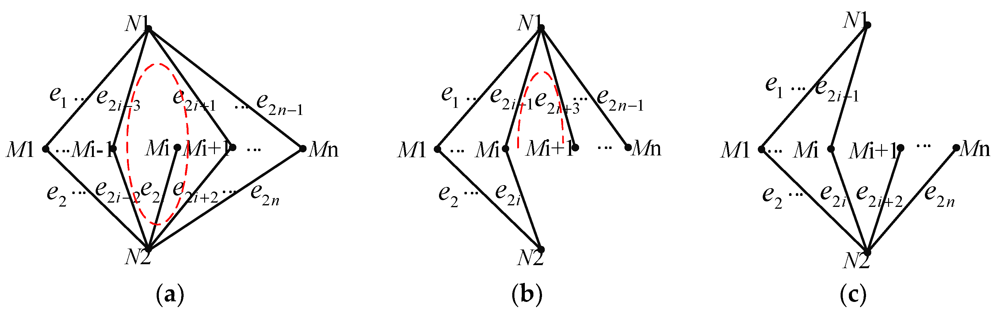
When the two circuit breakers of one parallel line are both closed, only elements corresponding to the first parallel connections before and after the fault point have a value of 1.

(2)

When one circuit breaker of one parallel line is closed, only the elements corresponding to the first ATP before and after the fault point have a value of 1.

(3)

When one circuit breaker at the SS is open, the two elements of the first column have a value of 1.

The indications of $A_P$ and $I_R$ are as shown in

Table 1. Indication of two matrices.

$A_{Pi}=0$		$A_{Pi}=1$
$I_{Rij}=0$	$I_{Rij}=1$	$I_{Rij}=0$	$I_{Rij}=1$
uncertain	uncertain	no-fault	fault

.

Thus, we formed a fault state matrix to reflect the fault state according to the parallel state matrix and the current state matrix as follows

$$I_{\mathrm{Q}}=A_P\otimes I_R={\left[\begin{array}{llll}{Q}_{C1}\hfill & Q_{C2}\hfill & \cdots \hfill & Q_{Cn}\hfill \\ Q_{F1}\hfill & Q_{F2}\hfill & \cdots \hfill & Q_{Fn}\hfill \end{array}\right]}_{2\times n}$$

(20)

where $\otimes$ denotes $I_{\mathrm{Q}1j}=A_{Pj}{I}_{R1j}$($Q_{Ci}=e_1\cap e_2\cap R_{Ci}$), $I_{\mathrm{Q}2j}=A_{Pj}{I}_{R2j}$($Q_{Fi}=e_1\cap e_2\cap R_{Fi}$). Therefore, the value 1 element in the matrix means that the up and down lines are in parallel connection at the ATP and the up and down currents are not equal.

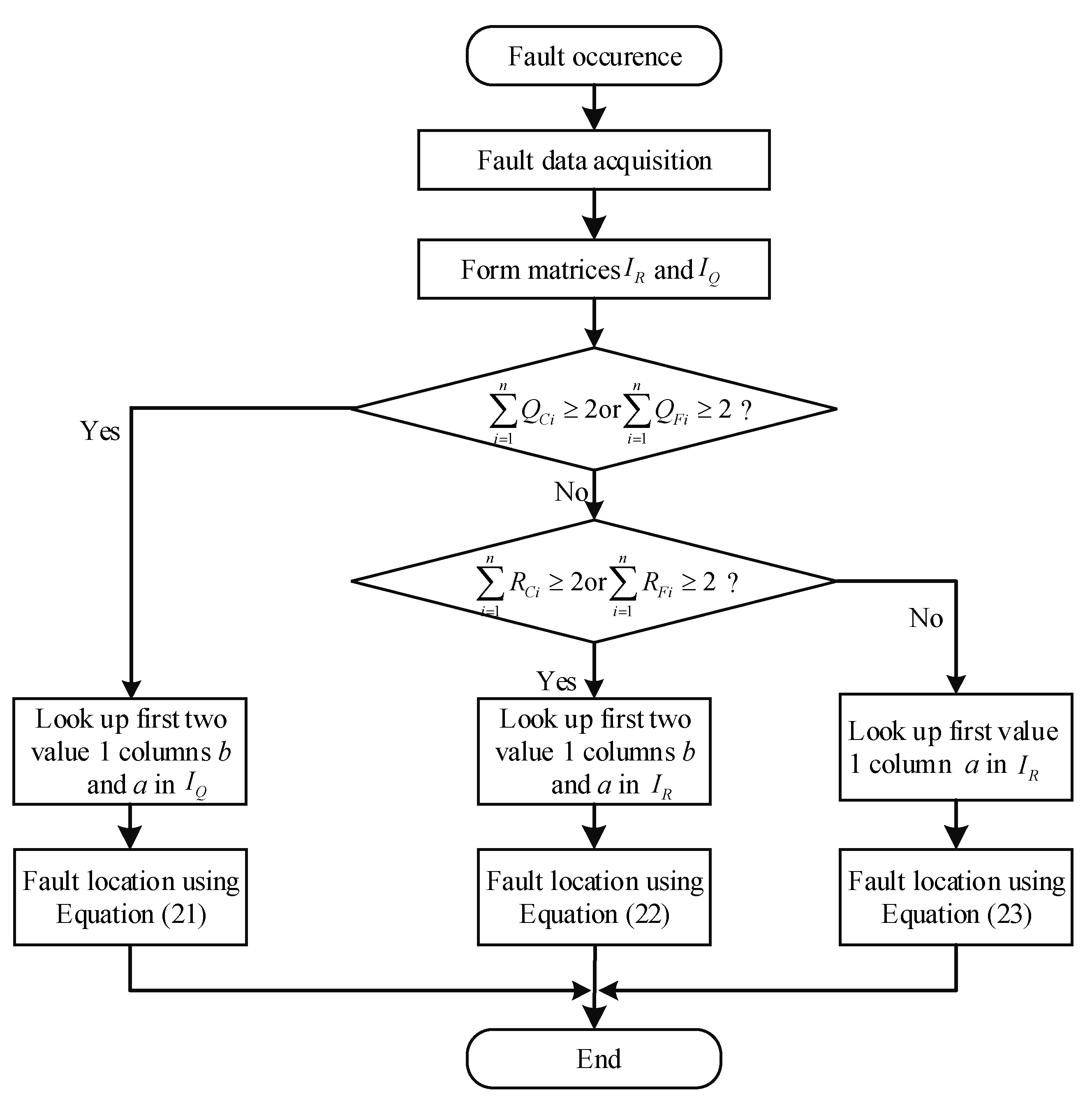
4.2. Identification of Faulted Section and Fault Location Scheme

According to the discussion in Section 3, we need to identify the faulted section in three feeding conditions, then we can use the corresponding fault location methods. After a fault occurs, the fault data are acquired synchronously and then the ATP data are transmitted to the SS [8] to form the current state matrix and fault state matrix. Finally, we use the following steps to obtain the fault distance.

(1) Check if the fault is in a UDP feeding section. In this condition, there are at least two columns containing a value 1 element in $I_{\mathrm{Q}}$, i.e., ${\displaystyle \sum _{i=1}^n{Q}_{Ci}}\ge 2 \mathrm{or} {\displaystyle \sum _{i=1}^n{Q}_{Fi}}\ge 2$. We look up from column n to 1 to find the first two columns containing value 1 element in $I_{\mathrm{Q}}$. Suppose the first column is b and the second column is a, this indicates the faulted section between ATPa and ATPb is in a UDP feeding condition; therefore, we use Equation (11) to calculate the distance $x_1$ from the fault point to ATPa, then we get the fault distance $L_x$ from the fault point to the SS as follows

$$L_x={\displaystyle \sum _{i=1}^{a-1}{D}_i}+x_1$$

(21)

(2) Check if the fault is a C-R or F-R fault in a SLAT feeding section. In this condition, there are at least two columns containing a value 1 element in $I_R$, i.e., ${\displaystyle \sum _{i=1}^n{R}_{Ci}}\ge 2$ and ${\displaystyle \sum _{i=1}^n{R}_{Fi}}\ge 2$. In this condition, we look up from column n to 1 to find the first two columns containing a value 1 element in $I_R$. Suppose the first column is b and the second column is a, this indicates the faulted section between ATPa and ATPb is in a SLAT feeding condition; therefore, we use Equation (13) to calculate the distance $x_2$ from the fault point to the ATPa, then we get the fault distance $L_x$ from the fault point to the SS as follows

$$L_x={\displaystyle \sum _{i=1}^{a-1}{D}_i}+x_2$$

(22)

(3) If the above two steps are not satisfied, we use the reactance method to locate the fault. We look up from column n to 1 to find the first column containing a value 1 element in $I_R$. Suppose the first column is a, this indicates that the faulted section begins from ATPa. Meanwhile, $R_{Ca}=1$ and $R_{Fa}=1$ indicate a C-F fault, only $R_{Ca}=1$ indicates a C-R fault, and only $R_{Fa}=1$ indicates a F-R fault. Therefore, we use Equation (14) to calculate the distance $x_3$ from the fault point to the ATPa, then we get the fault distance $L_x$ from the fault point to the SS as follows

$$L_x={\displaystyle \sum _{i=1}^{a-1}{D}_i}+x_3$$

(23)

Figure 9 shows the flowchart of the proposed fault location scheme.

5. Simulation and Analysis

We employed a railway system, as shown in Figure 1 to verify the effectiveness of the proposed scheme. The simulated railway system was built in a RTDS simulator. The RTDS simulator consists of the RSCAD software package and a proprietary hardware platform. RSCAD as used to create a detailed model of the simulated railway system [20]. The RTDS simulator’s hardware platform was used to perform simulation calculations. The simulated railway system parameters: $n=4$ (three AT sections: SS-ATP1 12 km, ATP1-ATP2 16 km, ATP2-ATP3 12 km), CB3 and CB8 are open, as shown in Figure 10.

We used distance relay [21] to trigger synchronous acquisition of the fault data. If a fault occurs, distance relay at the SS detects the fault and sends trigger signals to all fault location devices to obtain the synchronous measurements. To obtain accurate data, the fault voltages and currents were first prefiltered by second-order Butterworth digital filters (sampling frequency = 2400 Hz and cutoff frequency = 500 Hz), and then calculated by the modified full-cycle Discrete Fourier Transform (DFT) [22].

5.1. Case Analysis

Example 1.

Assume a F-R fault occurs at point k1 at 6 km from ATP1 as shown in Figure 10, the corresponding switch state matrix can be obtained as follows

$$A_{Q1}=\left[\begin{array}{llll}1\hfill & 0\hfill & 1\hfill & 1\hfill \\ 1\hfill & 1\hfill & 1\hfill & 0\hfill \end{array}\right]$$

(24)

Its parallel state matrix is

$$A_{P1}=\left[\begin{array}{llll}1\hfill & 0\hfill & 1\hfill & 0\hfill \end{array}\right]$$

(25)

The feeder current matrix is

$$I_{d1}=\left[\begin{array}{llll}0.224\hfill & 0.394\hfill & 0.120\hfill & 0.059\hfill \\ 1.312\hfill & 0.384\hfill & 2.833\hfill & 0.052\hfill \end{array}\right]kA$$

(26)

By comparing each element of$I_{d1}$with a given threshold of 200 A, we get the current state matrix:

$$I_{R1}=\left[\begin{array}{llll}1\hfill & 1\hfill & 0\hfill & 0\hfill \\ 1\hfill & 1\hfill & 1\hfill & 0\hfill \end{array}\right]$$

(27)

Therefore, the fault state matrix is

$$I_{Q1}=\left[\begin{array}{llll}1\hfill & 0\hfill & 0\hfill & 0\hfill \\ 1\hfill & 0\hfill & 1\hfill & 0\hfill \end{array}\right]$$

(28)

We can determine that the fault occurs in a UDP feeding section, because${\displaystyle \sum _{i=1}^4{Q}_{Fi}}=2$. It can be seen from Equation (27) that the feeding conditions of the faulted section cannot be identified by only using the fault current. However, we can derive the fault state matrix to identify the faulted section as shown in Equation (28). The fault occurs between the SS and ATP2 because the value 1 elements are in the first and third columns.

Example 2.

Assume a C-R fault occurs at point k2 at 8 km from ATP2 as shown in Figure 10. According to the above-mentioned solution, the corresponding fault state matrix is

$$I_{Q2}=\left[\begin{array}{llll}0\hfill & 0\hfill & 1\hfill & 0\hfill \\ 0\hfill & 0\hfill & 1\hfill & 0\hfill \end{array}\right]$$

(29)

We can determine that the fault does not occur in a UDP feeding section, because${\displaystyle \sum _{i=1}^4{Q}_{Ti}}<2$and${\displaystyle \sum _{i=1}^4{Q}_{Fi}}<2$. Meanwhile, the current state matrix is

$$I_{R2}=\left[\begin{array}{llll}0\hfill & 0\hfill & 1\hfill & 1\hfill \\ 0\hfill & 0\hfill & 1\hfill & 1\hfill \end{array}\right]$$

(30)

We can determine that the fault occurs in a SLAT feeding section, because${\displaystyle \sum _{i=1}^4{R}_{Ci}}>2$,${\displaystyle \sum _{i=1}^4{R}_{Fi}}>2$. In addition, the fault occurs between ATP2 and ATP3 because the first two elements with values of 1 are in the third and fourth columns.

Example 3.

Assume a C-F fault occurs at point k3 at 10 km from ATP2 as shown in Figure 10. We can obtain the current state matrix and fault state matrix as follows

$$I_{R3}=\left[\begin{array}{llll}0\hfill & 0\hfill & 1\hfill & 0\hfill \\ 0\hfill & 0\hfill & 1\hfill & 0\hfill \end{array}\right]$$

(31)

$$I_{Q3}=\left[\begin{array}{llll}0\hfill & 0\hfill & 1\hfill & 0\hfill \\ 0\hfill & 0\hfill & 1\hfill & 0\hfill \end{array}\right]$$

(32)

We can determine that it is a C-F fault in a SLTR feeding section, because${\displaystyle \sum _{i=1}^4{Q}_{Ci}}={\displaystyle \sum _{i=1}^4{Q}_{Fi}}=1$and${\displaystyle \sum _{i=1}^4{R}_{Ci}}={\displaystyle \sum _{i=1}^4{R}_{Fi}}=1$. Meanwhile, this indicates the fault occurs between ATP2 and ATP3 because the first value 1 element is in the third column.

The above analysis strongly proves that the proposed scheme can effectively identify the faulted section.

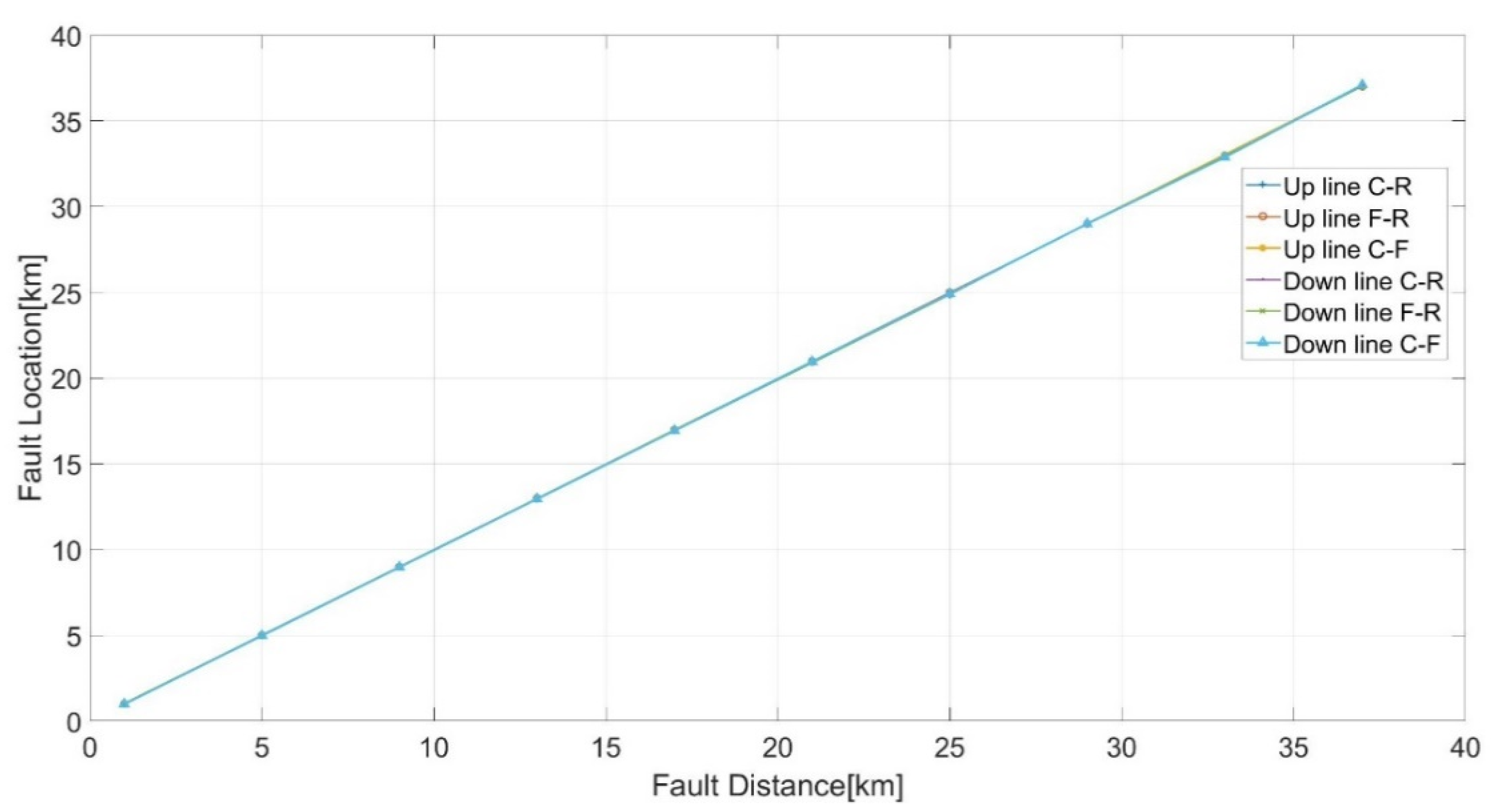
5.2. Results of Proposed Scheme

(a)

Impact of Fault Distance

To analyze the impacts of fault distance on the proposed scheme, faults at different points were simulated. The states of the circuit breakers are shown in Figure 10. The simulation results are shown in

Table 2. Results at different positions.

Fault Distance/km	Fault Location/km
	Up line			Down Line
	C-R	F-R	C-F	C-R	F-R	C-F
1	1.03	1.01	1.02	0.99	0.99	0.99
5	5.00	5.00	5.00	4.98	4.97	4.98
9	8.97	9.00	8.99	8.97	8.96	8.97
13	12.94	13.00	12.97	12.96	12.94	12.95
17	16.92	16.99	16.98	16.96	16.91	16.94
21	20.89	20.99	20.94	20.96	20.88	20.93
25	24.86	24.99	24.93	24.96	24.86	24.92
29	29.00	29.00	29.00	29.00	29.00	29.00
33	32.90	32.98	33.02	32.91	32.96	32.88
37	37.03	37.01	37.06	37.08	37.01	37.10

and Figure 11. We can see that the proposed scheme can achieve fault location accurately for all types of faults at different positions.

(b)

Impact of the Feeding Condition

To investigate the impact of the feeding condition on the proposed scheme, we first opened or closed the corresponding circuit breakers of the simulated railway system to form different feeding conditions, and then simulated faults at different positions in order to examine the proposed scheme.

Table 3. Results for typical feeding conditions.

No.	Switch State Matrix	k1		k2		k3
		Faulted Section	Fault Location/km	Faulted Section	Fault Location/km	Faulted Section	Fault Location/km
1	$\left[\begin{array}{llll}1\hfill & 1\hfill & 1\hfill & 1\hfill \\ 1\hfill & 1\hfill & 1\hfill & 1\hfill \end{array}\right]$	ATP1-ATP2	16.98	ATP2-ATP3	33.02	ATP2-ATP3	32.96
2	$\left[\begin{array}{llll}1\hfill & 0\hfill & 0\hfill & 1\hfill \\ 1\hfill & 0\hfill & 0\hfill & 1\hfill \end{array}\right]$	SS-ATP3	16.94	SS-ATP3	32.85	SS-ATP3	32.96
3	$\left[\begin{array}{llll}1\hfill & 1\hfill & 1\hfill & 1\hfill \\ 0\hfill & 0\hfill & 0\hfill & 0\hfill \end{array}\right]$	ATP1-ATP2	17.06	ATP2-ATP3	33.05	-	-
4	$\left[\begin{array}{llll}1\hfill & 0\hfill & 0\hfill & 0\hfill \\ 1\hfill & 0\hfill & 0\hfill & 0\hfill \end{array}\right]$	SS-ATP3	17.08	SS-ATP3	33.03	SS-ATP3	32.95
5	$\left[\begin{array}{llll}1\hfill & 1\hfill & 1\hfill & 1\hfill \\ 1\hfill & 1\hfill & 1\hfill & 0\hfill \end{array}\right]$	ATP1-ATP2	16.98	ATP2-ATP3	33.11	ATP2-ATP3	32.87
6	$\left[\begin{array}{llll}1\hfill & 1\hfill & 1\hfill & 1\hfill \\ 1\hfill & 0\hfill & 1\hfill & 1\hfill \end{array}\right]$	SS-ATP2	17.00	ATP2-ATP3	33.02	ATP2-ATP3	33.01
7	$\left[\begin{array}{llll}1\hfill & 1\hfill & 1\hfill & 0\hfill \\ 1\hfill & 1\hfill & 0\hfill & 1\hfill \end{array}\right]$	ATP1-ATP2	17.12	ATP2-ATP3	33.02	ATP1-ATP3	33.02
8	$\left[\begin{array}{llll}1\hfill & 0\hfill & 1\hfill & 1\hfill \\ 1\hfill & 1\hfill & 1\hfill & 0\hfill \end{array}\right]$	SS-ATP2	16.99	ATP2-ATP3	32.90	ATP2-ATP3	32.88
9	$\left[\begin{array}{llll}1\hfill & 1\hfill & 1\hfill & 0\hfill \\ 1\hfill & 1\hfill & 1\hfill & 0\hfill \end{array}\right]$	ATP1-ATP2	16.97	ATP2-ATP3	33.02	ATP2-ATP3	32.87
10	$\left[\begin{array}{llll}1\hfill & 1\hfill & 0\hfill & 1\hfill \\ 1\hfill & 1\hfill & 0\hfill & 1\hfill \end{array}\right]$	ATP1-ATP3	16.94	ATP1-ATP3	33.01	ATP1-ATP3	32.99
11	$\left[\begin{array}{llll}1\hfill & 0\hfill & 1\hfill & 0\hfill \\ 1\hfill & 1\hfill & 0\hfill & 1\hfill \end{array}\right]$	SS-ATP2	16.96	ATP2-ATP3	32.98	ATP1-ATP3	33.00
12	$\left[\begin{array}{llll}1\hfill & 1\hfill & 1\hfill & 0\hfill \\ 0\hfill & 1\hfill & 0\hfill & 1\hfill \end{array}\right]$	ATP1-ATP2	17.06	ATP2-ATP3	32.90	ATP1-ATP3	32.97
13	$\left[\begin{array}{llll}1\hfill & 0\hfill & 0\hfill & 0\hfill \\ 1\hfill & 1\hfill & 1\hfill & 1\hfill \end{array}\right]$	SS-ATP3	17.01	SS-ATP3	32.92	ATP2-ATP3	32.87
14	$\left[\begin{array}{llll}1\hfill & 1\hfill & 0\hfill & 0\hfill \\ 1\hfill & 1\hfill & 1\hfill & 0\hfill \end{array}\right]$	ATP1-ATP3	16.98	ATP1-ATP3	32.92	ATP2-ATP3	32.89
15	$\left[\begin{array}{llll}1\hfill & 0\hfill & 0\hfill & 1\hfill \\ 1\hfill & 1\hfill & 0\hfill & 0\hfill \end{array}\right]$	SS-ATP3	17.12	SS-ATP3	33.10	ATP1-ATP3	32.97

shows the results of fault location in typical feeding condition. The positions of k1, k2, k3 are shown in Figure 10, and fault distance is 5 km from the previous ATP, i.e., 17 km, 33 km, 33 km, respectively, from SS. In Table 3, the switch state matrices in column 2 reflect the states of all circuit breakers, which form different feeding conditions in the AARS. The faulted sections in column 3, 5 and 7 are identified by using the methods in Section 4.2. Columns 4, 6 and 8 show the fault location results for different feeding condition.

Table 3 shows the fault location results at different positions in 15 typical feeding conditions of the AARS. Take the simulation results in row 8 as an example: in row 8, k1 is in the faulted section from SS to ATP2 with UDP feeding condition, k2 is in the faulted section from ATP2 to ATP3 with SLAT feeding condition, k3 is in the faulted section from ATP2 to ATP3 with SLTR feeding condition. We can see that the proposed scheme effectively identifies and locates all faults in different feeding conditions. Thus, the proposed scheme locates faults by identifying the feeding conditions of faulted sections and choosing the relative fault location methods, so as not to match each of feeding conditions of the whole railway system, therefore, the scheme performs well regardless of the feeding conditions of the AARS.

6. Conclusions

To obtain accurate fault location in different conditions, this paper proposes a generalized fault location scheme for AARS that considers the relationship between the fault current distribution and feeding condition according to the characteristics of the fault state matrix. The proposed scheme deals effectively with the negative influence of the feeding condition on fault location. Meanwhile, the proposed scheme improves the up and down current ratio method, neutral current ratio method and reactance method for long-section feeding conditions. The simulation results show the effectiveness of the proposed scheme.

References

1. Zhou, Y.; Xu, G.; Chen, Y. Fault Location in Power Electrical Traction Line System. Energies 2012, 5, 5002–5018. [Google Scholar] [CrossRef]
2. Yu, C.; Chang, L.; Cho, J. New Fault Impedance Computations for Unsychronized Two-Terminal Fault-Location Computations. IEEE Trans. Power Del. 2011, 26, 2879–2881. [Google Scholar] [CrossRef]
3. Bains, T.; Zadeh, M. Supplementary Impedance-Based Fault Location Algorithm for Series Compensated Lines. IEEE Trans. Power Del. 2015, 31, 334–342. [Google Scholar] [CrossRef]
4. Zhu, J.; Lubkeman, D.; Girgis, A. Automated Fault Location and Diagnosis on Electric Power Distribution Feeders. IEEE Trans. Power Del. 1997, 12, 801–808. [Google Scholar]
5. Dashti, R.; Tahavori, M.; Daisy, M.; Shaker, H. A New Matching Algorithm for Fault Section Estimation in Power Distribution Networks. In Proceedings of the 2018 International Symposium on Advanced Electrical and Communication Technologies (ISAECT), Rabat, Morocco, 21–23 November 2018; pp. 1–4. [Google Scholar]
6. Liao, Y. Generalized Fault-Location Methods for Overhead Electric Distribution Systems. IEEE Trans. Power Del. 2011, 26, 53–64. [Google Scholar] [CrossRef]
7. Han, Z.; Li, S.; Liu, S.; Gao, S. A Reactance-Based Fault Location Method for Overhead Lines of AC Electrified Railway. IEEE Trans. Power Del. 2020. [Google Scholar] [CrossRef]
8. Fujie, H.; Miura, A. Fault Location System in Autotransformer Feeding Circuit of AC Electric Railways. Electr. Eng. Jpn. 1976, 5, 96–105. [Google Scholar] [CrossRef]
9. Gao, S.; Huang, W. Principle and Application of a New Type Microprocessor-based Fault Locator for AT Feeding Traction System. In Proceedings of the Sixth International Conference on Developments in Power System Protection, Nottingham, UK, 25–27 March 1997; pp. 323–326. [Google Scholar]
10. Wang, C.; Yin, X. Comprehensive Revisions on Fault-Location Algorithm Suitable for Dedicated Passenger Line of High-Speed Electrified Railway. IEEE Trans. Power Del. 2012, 27, 2415–2417. [Google Scholar] [CrossRef]
11. Serrano, J.; Platero, C.; López-Toledo, M.; Granizo, R. A New Method of Ground Fault Location in 2 × 25 kV Railway Power Supply Systems. Energies 2017, 10, 340. [Google Scholar] [CrossRef] [Green Version]
12. Cho, G.; Kim, C.; Kim, M.; Kim, D.-H.; Heo, S.-H.; Min, M.-H.; An, T.-P. A Novel Fault-Location Algorithm for AC Parallel Autotransformer Feeding System. IEEE Trans. Power Del. 2019, 34, 475–485. [Google Scholar] [CrossRef]
13. Duan, J.J.; Xue, Y.D.; Xu, B.Y.; Sun, B. Study on technology of traveling wave method fault location in traction power supply system. In Proceedings of the 10th IET International Conference on Developments in Power System Protection (DPSP 2010). Managing the Change, Manchester, UK, 29 March–1 April 2010; pp. 1–5. [Google Scholar]
14. Zhang, D.; Wu, M.; Xia, M. Study on Traveling Wave Fault Location Device for Electric Railway Catenary System Based on DSP. In Proceedings of the 2009 International Conference on Sustainable Power Generation and Supply, Nanjing, China, 6–7 April 2009; pp. 1–4. [Google Scholar]
15. Xia, M.; Wu, M. Traveling Wave Fault Location Scheme for Jing-Jin Dedicated Passenger Line Electric Railway Traction System. In Proceedings of the 2009 International Conference on Power Engineering, Energy and Electrical Drives, Lisbon, Portugal, 18–20 March 2009; pp. 447–449. [Google Scholar]
16. Oura, Y.; Mochinaga, Y.; Nagasawa, H. Railway Electric Power Feeding systems. Jpn. Railw. Transp. Rev. 1998, 16, 48–58. [Google Scholar]
17. Zhao, T.; Wu, M. Electric Power Characteristics of All-Parallel AT Traction Power Supply System. In Proceedings of the 2011 International Conference on Transportation, Mechanical, and Electrical Engineering (TMEE), Changchun, China, 16–18 December 2011; pp. 895–898. [Google Scholar]
18. Zhang, S.; Yan, Y.; Bao, W.; Guo, S.; Jiang, J.; Ma, M. Network Topology Identification Algorithm Based on Adjacency Matrix. In Proceedings of the 2017 IEEE Innovative Smart Grid Technologies—Asia (ISGT-Asia), Auckland, New Zealand, 4–7 December 2017; pp. 1–5. [Google Scholar]
19. Wang, Y.; Liu, Z.; Yan, W. Algorithms for Random Adjacency Matrixes Generation Used for Scheduling Algorithms Test. In Proceedings of the 2010 International Conference on Machine Vision and Human-machine Interface, Kaifeng, China, 24–25 April 2010; pp. 422–424. [Google Scholar]
20. Han, Z.; Zhang, Y.; Liu, S.; Gao, S. Modeling and Simulation for Traction Power Supply System of High-Speed Railway. In Proceedings of the 2011 Asia-Pacific Power and Energy Engineering Conference (APPEEC), Wuhan, China, 25–28 March 2011; pp. 1–4. [Google Scholar]
21. Han, Z.; Liu, S.; Gao, S.; Bo, Z. Protection Scheme for China High-Speed Railway. In Proceedings of the 10th IET International Conference on Developments in Power System Protection (DPSP 2010). Managing the Change, Manchester, UK, 29 March–1 April 2010; pp. 1–5. [Google Scholar]
22. Gu, J.; Yu, S. Removal of DC Offset in Current and Voltage Signals Using a Novel Fourier Filter Algorithm. IEEE Trans. Power Del. 2000, 15, 73–79. [Google Scholar]
Figure 1. Schematic diagram of an all-parallel autotransformer railway system (AARS).
Energies 13 04081 g001
Figure 2. Current distribution in the up-down parallel (UDP) feeding condition.
Energies 13 04081 g002
Figure 3. Current distribution in a single-line AT (SLAT) feeding condition.
Energies 13 04081 g003
Figure 4. Current distribution in a single-line track return (SLTR) feeding condition.
Energies 13 04081 g004
Figure 5. Measured reactance with fault distance.
Energies 13 04081 g005
Figure 6. Single-line diagram of AARS.
Energies 13 04081 g006
Figure 7. AARS connection diagram. N 1 , N 2 , the generalized nodes.
Energies 13 04081 g007
Figure 8. Connection diagram in different feeding conditions (a) UDP (b) SLAT (c) SLTR.
Energies 13 04081 g008
Figure 9. Flowchart of the proposed fault location scheme.
Energies 13 04081 g009
Figure 10. Simulated railway system.
Energies 13 04081 g010
Figure 11. Fault location results vs. fault distance.
Energies 13 04081 g011