Article

Density Difference Grid Design in a Point-Mass Filter

by
Jakub Matoušek
,
Jindřich Duník
*,† and
Ondřej Straka
Department of Cybernetics, University of West Bohemia, Univerzitní 8, 306 14 Pilsen, Czech Republic
*
Author to whom correspondence should be addressed.
These authors contributed equally to this work.
Energies 2020, 13(16), 4080; https://doi.org/10.3390/en13164080
Submission received: 22 June 2020 / Revised: 17 July 2020 / Accepted: 3 August 2020 / Published: 6 August 2020
(This article belongs to the Special Issue Advanced Control Design and Fault Diagnosis)

Abstract

:
The paper deals with the Bayesian state estimation of nonlinear stochastic dynamic systems. The stress is laid on the point-mass filter, solving the Bayesian recursive relations for the state estimate conditional density computation using the deterministic grid-based numerical integration method. In particular, the grid design is discussed and the novel density difference grid is proposed. The proposed grid design covers such regions of the state-space where the conditional density is significantly spatially varying, by the dense grid. In other regions, a sparse grid is used to keep the computational complexity low. The proposed grid design is thoroughly discussed, analyzed, and illustrated in a numerical study.

1. Introduction

State estimation of nonlinear discrete-time stochastic dynamic systems from noisy or incomplete measurements has been a subject of considerable research interest. The topic plays an important role in signal processing, control, and fault detection of both small and large scale systems in virtually all fields of industry [1] including power generation and transmission, battery live prediction [2,3,4,5,6,7,8], automotive [9,10], navigation [11,12], speech and image processing etc. State estimation methods has also become important in non-technical fields including, for example, economics, biology, or weather forecasting.
In the Bayesian framework, a general solution to the state estimation problem is given by the Bayesian recursive relations (BRRs), which compute the probability density functions (PDFs) of the state conditioned on the measurements. The conditional PDFs fully describe the estimate of the immeasurable state of a nonlinear or non-Gaussian stochastic dynamic system. Besides a set of linear models leading e.g., to the Kalman filter (KF), the BRRs are not analytically tractable and an approximation in their solution must be used. The resulting approximate methods can be divided with respect to the validity of the resulting estimates into global and local filters [13,14].
The local filters provide computationally efficient estimates in the form of the conditional mean and covariance matrix with potentially limited performance due to inherent underlying Gaussian assumption, which is not always realistic (as the first two moments usually do not represent a full description of the immeasurable state). These filters are represented by the extended Kalman filter, the unscented Kalman filter, or the stochastic integration filter [14,15,16,17,18].
As opposed to the local filters, the global filters provide estimates in the form of conditional PDFs without any assumption on the conditional distribution family. The global filters are capable of estimating the state of a strongly nonlinear or non-Gaussian system but usually at the cost of higher computational demands. Among these, the Gaussian sum filter [19], the particle filter [20], and the point-mass filter [21,22,23,24] have attracted a considerable attention.
The point-mass filter (PMF) considered in this paper is based on a numerical solution to the BRRs using deterministic grid-based numerical integration rules, which means the BRRs are solved and the conditional PDF is computed at the grid points only. Although a conceptual design of the PMF is known from the seventies [13], an application in the terrain-aided navigation (TAN) [22] is reported as late as the nineties mainly because of the computational complexity of the filter. Therefore, since the development of the PMF, extensive attention is devoted to the efficient filter design reducing the computational complexity. In the literature, two main directions of reduction can be found;
  • Design of the Rao-Blackwellized (or marginalized) PMF [23,25],
  • Efficient convolution in the PMF prediction step [21,22,24,26,27,28,29].
The former approach is based on the decomposition of the state vector into two parts; nonlinearly and linearly modeled. As a consequence, just the nonlinearly modeled part of the state is estimated by the computationally expensive PMF and the remaining part of the state vector is estimated by a set of computationally cheap KFs. The Rao–Blackwellized PMF is thus suitable for possibly high-dimensional models with specific conditionally linear structure and Gaussian noises. The latter approach typically does not restrict the class of the allowed state-space models, but it rather focuses on computationally effective implementation of the convolution, as the most demanding step, in the prediction of the PMF.
Recently, a novel method for the efficient convolution, based on the the density-specific grid (DSG) design, was proposed [24]. Compared to other methods (typically assuming one equidistant grid), the DSG assumes two different grids (each with different properties);
  • Denser grid supporting symmetrical vicinity of the conditional PDF mean (where a higher volume of the conditional PDF is expected),
  • Sparser grid supporting conditional PDF tail region (where a marginal volume of the conditional PDF is expected).
The DSG brings significant improvement to the estimation quality especially for unimodal and rather symmetric conditional PDFs with light tails. If the density is multimodal, heavy-tailed, or heavy-skewed, the benefit of the DSG is marginal.
The goal of the paper is, thus, to design an advanced version of the DSG, further denoted as the density difference grid (DDG). The proposed DDG is based on the differentiation of the conditional PDF at the sparse grid, which allows accurate determination of the regions with a significant spatial change of the PDF. In these regions, the denser grid is created to reasonably well capture the PDF shape. As a consequence, the DDG has an ability to better approximate asymmetric, heavy-tailed, and multi-modal PDFs, i.e., the PDFs with dominant higher-order moments, with a negligible increase of the overall PMF computational complexity.
The rest of the paper is organized as follows. In Section 2, the system description and a brief introduction to the Bayesian state estimation is presented. Then, in Section 3, the points-mass filter is overviewed. This overview is accompanied with a short recapitulation of the state-of-the-art grid designs. Section 4 proposes a novel DDG design and Section 5 shows the DDG performance in a numerical study. Finally, concluding remarks are drawn in Section 6.

2. System Description and Bayesian State Estimation

Let the following discrete-time state-space model of a nonlinear stochastic dynamic system
x k + 1 = f k ( x k , u k ) + w k , k = 0 , 1 , 2 , , T ,
z k = h k ( x k ) + v k , k = 0 , 1 , 2 , , T ,
be considered, where the vectors x k R n x , u k R n u , and  z k R n z represent the unknown state of the system and the known input and measurement at time instant k, respectively. The state and measurement functions f k : R n x × n u R n x and h k : R n x R n z are known general transformations. Particular realizations of the state and measurement noises w k and v k are unknown, but their PDFs, i.e., the state noise PDF p ( w k ) and the measurement noise PDF p ( v k ) , are supposed to be known and independent of the known initial state PDF p ( x 0 ) .
The goal of the state estimation, particularly of the filtering, is to find an estimate of the state x k conditioned on all measurements z k = [ z 0 , z 1 , , z k ] up to the time instant k. In the Bayesian framework, the state estimate in the form of the conditional PDF p ( x k | z k ) , k , is sought. Note that, considering the model (1), (2), the state transition PDF and the BRRs (3)–(5) should be conditioned also on available sequence of the input u k , k . However, for the sake of notational simplicity, the input signal is assumed to be implicitly part of the condition and it is not explicitly stated, i.e.,  p ( x k + 1 | x k ) = p ( x k + 1 | x k ; u k ) , p ( x k | z k ) = p ( x k | z k ; u k 1 ) , and  p ( x k + 1 | z k ) = p ( x k + 1 | z k ; u k ) .
The Bayesian state estimator design stems from the solution of the Bayesian recursive relations (BRRs) for the recursive computation of the conditional PDFs [15]
p ( x k | z k ) = p ( x k , z k | z k 1 ) p ( z k | z k 1 ) = p ( x k | z k 1 ) p ( z k | x k ) p ( z k | z k 1 ) ,
p ( x k | z k 1 ) = p ( x k | x k 1 ) p ( x k 1 | z k 1 ) d x k 1 ,
where p ( x k | z k ) is the filtering PDF computed by the Bayes’ rule (3) and p ( x k | z k 1 ) is the one-step predictive PDF computed by the Chapman–Kolmogorov Equation (4). The PDFs p ( x k | x k 1 ) and p ( z k | x k ) are the state transition PDF obtained from system dynamics (1) and the measurement PDF obtained from measurement Equation (2), respectively. The PDF
p ( z k | z k 1 ) = p ( x k | z k 1 ) p ( z k | x k ) d x k
is the one-step predictive PDF of the measurement. The recursion (3), (4) starts from the initial PDF, i.e.,  p ( x 0 | z 1 ) = p ( x 0 ) .

3. Point-Mass Filter Summary and Grid Designs

The PMF is based on the numerical solution to BRRs using the deterministic integration rules. As a consequence, a significant part of the (continuous) state-space is approximated by the grid of isolated points in which the conditional PDFs are computed. The PDF evaluated at the grid points is denoted as the point-mass PDF or, alternatively, as the point-mass density (PMD).

3.1. Point-Mass PDF Approximation

Approximation of a conditional PDF p ( x k | z m ) , where m = k for the filtering PDF (3) and m = k 1 for the predictive PDF (4), by a piece-wise constant PMD p ^ ( x k | z m ; ξ k ) defined at the set of the discrete grid points ξ k = { ξ k ( i ) } i = 1 N , ξ k ( i ) R n x , is as follows
p ( x k | z m ) p ^ ( x k | z m ; ξ k ) i = 1 N P k | m ( ξ k ( i ) ) S { x k ; ξ k ( i ) , Δ k } ,
with
  • P k | m ( ξ k ( i ) ) = c k P ˜ k | m ( ξ k ( i ) ) , where P ˜ k | m ( ξ k ( i ) ) = p ( ξ k ( i ) | z m ) is the value of the conditional PDF p ( x k | z m ) evaluated at i-th grid point ξ k ( i ) , c k = δ k i = 1 N P ˜ k | m ( ξ k ( i ) ) is a normalization constant, and  δ k is a volume of the i-th point neighbourhood defined below,
  • Δ k = [ Δ k ( 1 ) , Δ k ( 2 ) , , Δ k ( n x ) ] T defines a (hyper-)rectangular neighbourhood of a grid point ξ k ( i ) , where the PDF p ( x k | z m ) is assumed to be constant and has value P k | m ( ξ k ( i ) ) , and
  • S { x k ; ξ k ( i ) , Δ k } is the selection function defined as
    S { x k ; ξ k ( i ) , Δ k } = 1 ,
    if x k ( j ) [ ξ k ( i ) ( j ) Δ k ( j ) 2 , ξ k ( i ) ( j ) + Δ k ( j ) 2 ] for j = 1 , 2 , , n x , and
    S { x k ; ξ k ( i ) , Δ k } = 0 ,
    otherwise, so that
    S { x k ; ξ k ( i ) } d x k = Δ k ( 1 ) × Δ k ( 2 ) × × Δ k ( n x ) = δ k .
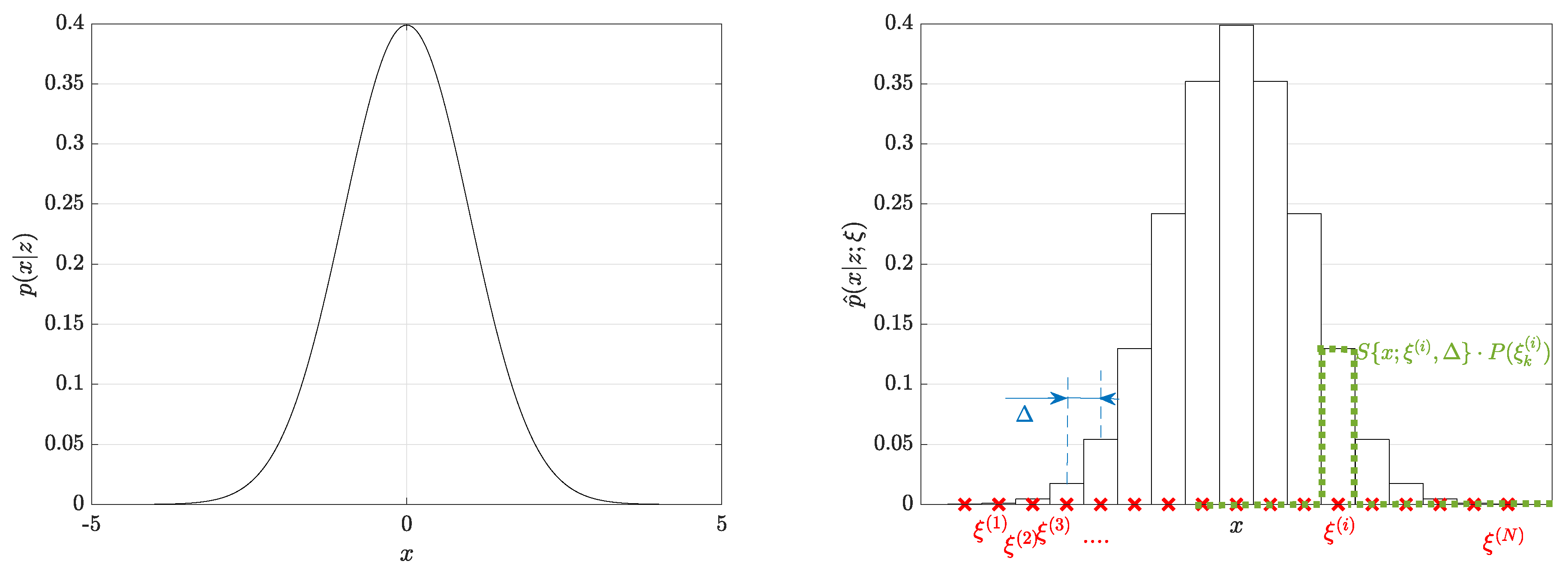
Note that in (6)–(9) the notation x ( j ) meaning the j-th element of the vector x was used. Illustration of the point-mass PDF approximation (6) with omitted time indices is shown in Figure 1. The point-mass density (6) can be, thus, interpreted as a sum of weighted uniform distributions. Another interpretations, such as the a sum of the Dirac delta functions, can be found in [22,26].

3.2. Point-Mass Filter Algorithm

The basic algorithm of the point-mass filter (PMF) can be summarised by the following Algorithm 1 [26,30]:
Algorithm 1: Point-Mass Filter
  • Initialization: Set k = 0 , construct the initial grid of points { ξ 0 ( i ) } i = 0 N , and define the initial point-mass PDF
    p ^ ( x 0 | z 1 ; ξ 0 ) = i = 1 N P 0 | 1 ( ξ 0 ( i ) ) S { x 0 ; ξ 0 ( i ) , Δ 0 } ,
    approximating the initial PDF p ( x 0 | z 1 ) ;
  • Measurement update: Compute the filtering point-mass PDF
    p ^ ( x k | z k ; ξ k ) = i = 1 N P k | k ( ξ k ( i ) ) S { x k ; ξ k ( i ) , Δ k } ,
    where
    P k | k ( ξ k ( i ) ) = p ( z k | x k = ξ k ( i ) ) P k | k 1 ( ξ k ( i ) ) i = 1 N p ( z k | x k = ξ k ( i ) ) P k | k 1 ( ξ k ( i ) ) δ k .
    is the value of the filtering PDF at i-th grid point;
  • Grid construction: Based on the filtering estimate (11) and the state Equation (1), construct the new grid of points { ξ k + 1 ( j ) } j = 1 N ;
  • Time update: Compute the predictive point-mass PDF at the new grid of points according to
    p ^ ( x k + 1 | z k ; ξ k + 1 ) = j = 1 N P k + 1 | k ( ξ k + 1 ( j ) ) S { x k + 1 ; ξ k + 1 ( j ) , Δ k + 1 } ,
    where the value of the predictive PDF at j-th grid point is
    P k + 1 | k ( ξ k + 1 ( j ) ) = i = 1 N p ( ξ k + 1 ( j ) | x k = ξ k ( i ) ) P k | k ( ξ k ( i ) ) δ k .
  • Set k = k + 1 and go to the step 2
For the sake of clarity, a detailed derivation of the PMF can be found in Appendix A. Note that the PMF filter provides estimates in the form of the PMD p ^ ( x k | z m ; ξ k ) approximating the conditional PDF p ( x k | z m ) . Assuming small grid point vicinity Δ k , the conditional moments, e.g., the mean and covariance matrix, can be easily computed according to [23]
x ^ PMD , k | m = i = 1 N δ k P k | m ( ξ k ( i ) ) ξ k ( i ) x ^ k | m = E [ x k | z m ] ,
P PMD , k | m = i = 1 N δ k P k | m ( ξ k ( i ) ) ( ξ k ( i ) x ^ k | m ) ( ξ k ( i ) x ^ k | m ) T P k | m = cov [ x k | z m ] ,
when required. The moments are, however, generally not needed for the PMF run.

3.3. Grid Design

A crucial part of the PMF design that is significantly affecting the filter estimation performance is a specification of the grid points before time update step (13) and, by extension, in the initialization (10).
When designing a grid, the number of grid points should be decided first. The more grid points N are considered, the better the accuracy of the density approximation can be achieved but at the cost of higher computational demands. Because of the convolution (13), (14), the computational complexity grows exponentially with N. Thus, the number of grid points is solely driven by the available computational capacity and required precision of the estimate (an analysis of ideal grid resolution can be found in [31]).
The grid should be designed to cover a significant region of the conditional PDFs support sufficiently well. Therefore, it is necessary to specify two grid characteristics
  • Region of the PDF support to be covered by the grid points,
  • Locations of grid points inside the region.
The former characteristic specification is common for all single-grid design techniques. The region R for the predictive PDF p ( x k + 1 | z k ) is (hyper-)rectangular and centred around the mean x ^ k + 1 | k = E [ x k + 1 | z k ] and is selected so that
R p ( x k + 1 | z k ) > P thr ,
where P thr is a user-defined threshold. Unfortunately, except for the initial condition, neither the predictive moments nor the predictive PDF is known at “Grid construction” step of Algorithm 1 (the PDF is to be computed in the subsequent step “Time update”). A reasonable approach is to compute the first two (approximate) predictive moments of the state
x ^ A , k + 1 | k = E [ x k + 1 | z k ] ,
P A , k + 1 | k = cov [ x k + 1 | z k ] ,
and to construct an approximate Gaussian predictive PDF
p A ( x k + 1 | z k ) = N { x k + 1 ; x ^ A , k + 1 | k , P A , k + 1 | k } ,
where the notation N { x ; x ^ , P } stands for the Gaussian PDF of the random variable x with the mean x ^ and the covariance matrix P (for simplicity, the random variable has same notation as its realization). Then, the sought region R can be found analogously to (17), where the approximate predictive PDF p A ( x k + 1 | z k ) (20) is used instead of the exact one p ( x k + 1 | z k ) . The predictive moments (18) and (19) are computed on the basis of known filtering moments (given by (15), (16), and (11)) and state equation (1). If the dynamics is nonlinear, approximate predictive moments can be computed e.g., by the unscented transformation or various numerical integration rules [16,32]. Note that, the approximate PDF (20) is used for the region R determination only.
The latter characteristic is specific for each grid design technique.

3.3.1. Equidistant Grid Design

The equidistant grid design [22] is a standard grid design technique, which covers the region R with equidistantly located points, i.e., the neighbourhood Δ k is the same for all grid points.

3.3.2. Density Specific Grid Design

The DSG design [24], is based on an unequally spaced placement of the fixed number of points over the PDF support R to be approximated. The main idea is to approximate the PDF, where the volume of the PDF is significant or significantly varying by a denser grid (as in this area, a slope of the PDF is expected to be significant) and the tail of the PDF by a sparser grid (as the tail is flat). Thus, the DSG design determines, besides the region R , also the hyper-rectangular subregion R in , where the grid is denser. The determination of the subregion again depends on the computed approximate predictive moments (18), (19).
As can be seen in [24], the DSG design significantly outperforms the standard equidistant grid design if the underlying conditional PDF is unimodal, rather symmetric, and light-tailed. If any of the mentioned properties are violated, the DSG benefit is marginal.

3.4. Goal of the Paper

The goal of the paper is to propose a novel unequally spaced grid design, called the density difference grid design (further abbreviated as DDG), which provides improved PMF estimation performance independently of the conditional PDF properties.

4. Density Difference Grid Design

The DDG design is based on the idea that such part of the support, where the conditional PDF is significantly spatially varying, should be covered by the dense grid (to sufficiently well capture PDF behavior). On the other hand, the remaining part of the support, i.e., the parts where the conditional PDF is almost flat, can be reasonably well approximated by the sparse grid. To realize this basic idea of the DDG, the following three steps should be performed:
  • Design of the sparse (outer) grid and evaluation of the predictive PMD at these grid points,
  • Differentiation of the “sparse” predictive PMD,
  • Design of the dense (inner) grids in the vicinity of such “sparse” grid points, which are associated with a large value of the difference.
Compared to the DSG design discussed in [24], the DDG design utilizes full information about the shape of the predictive PMD (and not only the moments) and also the denser (inner) grid need not be hyper-rectangular, which further improves the fit of the PDF and its grid support. The steps are particularized below.

4.1. Sparse Grid Design

The sparse grid design takes advantage of the PMF time-update, that the PDF value of a single point ξ k + 1 ( j ) can be counted independently of any other grid points. The sparse grid design is given by Algorithm 2:
Algorithm 2: DDG Sparse Grid
  • Define a threshold p thr below which the probability at a grid point is considered to be negligible and can be neglected. The threshold setting can be related to the computation precision of a given platform;
  • State Similarly as in the DSG design [24], compute the predictive moments x ^ A , k + 1 | k (18) and P A , k + 1 | k (19) and set the number of standard deviations (STDs) n σ of the marginal distributions of (20), which are used for specification of an a priori (hyper-)rectangular region R A to be covered by the grid points;
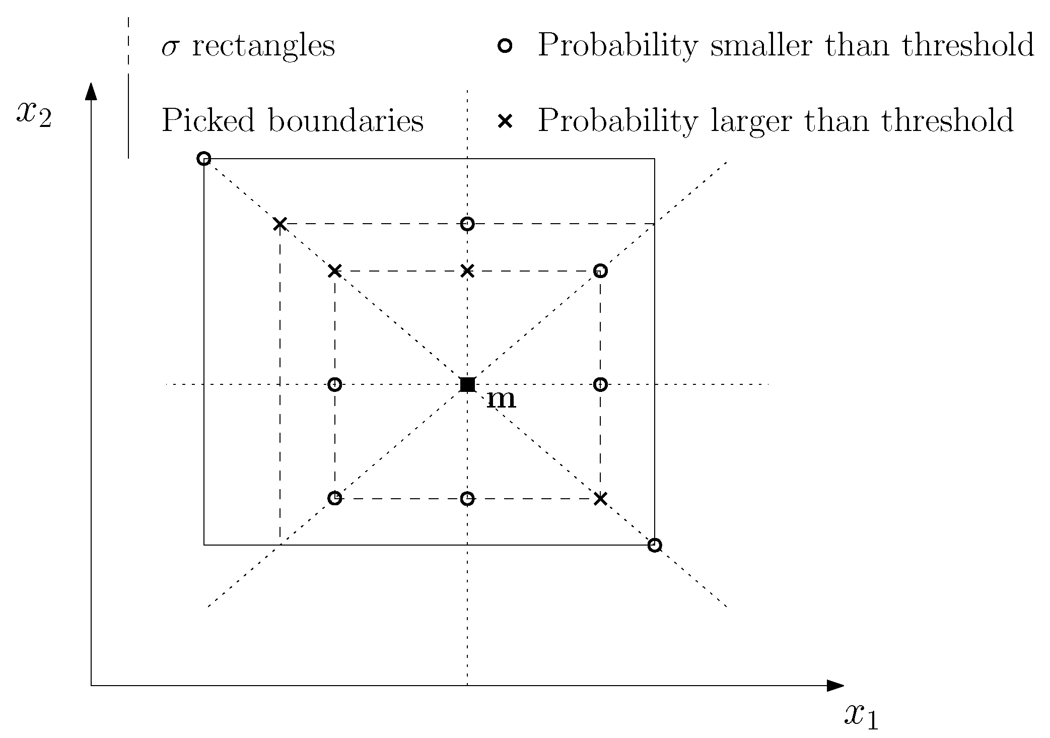
  • At the boundaries of the region R A select a small set of grid points and evaluate the predictive probability at these points. If the probability of the point is (significantly) below the threshold p thr , then the particular bound can be shifted towards the mean. On the other hand, if the probability of the point is (significantly) over the threshold p thr , then the particular bound can be shifted in an opposite direction from the mean. The shifted points are, then, re-evaluated;
  • When all boundary points are properly set, create the smallest possible hyper-rectangle defining R including all the boundary points. As a consequence, the resulting region R need not be symmetrical with respect to the mean;
  • Define a cardinality of the sparse grid N sparse and dense grid N dense = N N sparse . Fill the region R by equidistantly placed N sparse hyper-rectangular grid points { ξ sparse , k + 1 ( j ) } j = 1 N sparse (each sparse grid point is associated with a neighbourhood Δ sparse , k + 1 ). A reasonable choice N sparse = 1 3 N ;
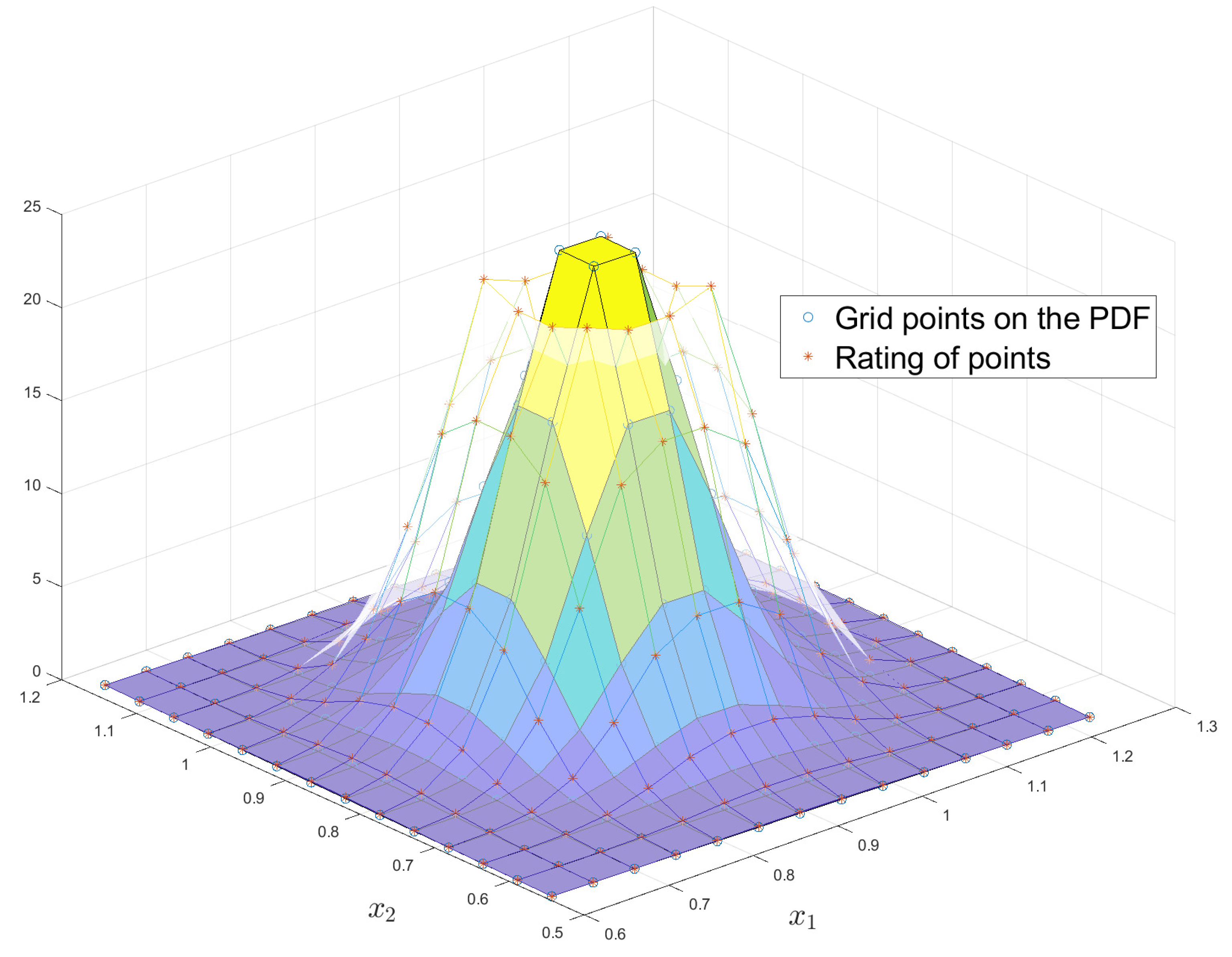
This algorithm is illustrated in Figure 2 for the two dimensional state-space.

4.2. Differentiation of Sparse Grid PMD

To find the state-space regions, where the conditional predictive PDF p ( x k + 1 | z k ) is expected to significantly spatially vary (i.e., the regions to be covered by the dense grid), the PMD evaluated at the sparse grid points is differenced according to Algorithm 3:
Algorithm 3: Sparse Grid PMD Differentiation
  • Compute the PMD for N sparse sparse grid points according to the convolution (14);
  • For each sparse grid point ξ sparse , k + 1 ( j ) compute the divided difference vector d k + 1 R 2 n x [14,33] according to
    d k + 1 ( j ) = [ P k + 1 | k ( ξ sparse , k + 1 ( j ) ) P k + 1 | k ( ξ sparse , k + 1 ( ı 1 ) ) ξ sparse , k + 1 ( j ) ξ sparse , k + 1 ( ı 1 ) 2 , , P k + 1 | k ( ξ sparse , k + 1 ( j ) ) P k + 1 | k ( ξ sparse , k + 1 ( ı 2 n x ) ) ξ sparse , k + 1 ( j ) ξ sparse , k + 1 ( ı 2 n x ) 2 ] ,
    where · 2 denotes the Euclidean norm and the index vector ı = [ ı 1 , ı 2 , , ı 2 n x ] is selected so that the closest neighbouring points of the j-th point ξ sparse , k + 1 ( j ) are chosen. It means two neighbouring points are selected for n x = 1 , four neighbouring points for n x = 2 , eight neighbouring points for n x = 3 , etc.;
  • Compute the grid points rating as a norm of the vector d k + 1 R 2 n x (21) according to
    d k + 1 ( j ) = d k + 1 ( j ) 2 , j ,
    which characterizes the overall spatial variability of the PDF in the vicinity of the j-th sparse grid point ξ sparse , k + 1 ( j ) .
This algorithm is illustrated in Figure 3 for the two dimensional state-space.

4.3. Design of Dense Grid

Having defined sparse grid points (Algorithm 2) and computed their difference rating (Algorithm 3), which in fact precisely denotes the state-space regions with significant change or variability of the conditional PDF, it is possible to construct the dense grid according to Algorithm 4:
Algorithm 4: Dense Grid Design
  • Sort the sparse grid points { ξ sparse , k + 1 ( j ) } j = 1 N sparse in a descending order according to their rating d k + 1 ( j )  (22);
  • Set the splitting ratio r (similarly as in the DSG design in [24]), which determines number of dense grid points r n x used for covering the vicinity of the j-th sparse grid ξ sparse , k + 1 ( j ) . Reasonable choice is r = { 2 , 3 } , but note that, the ratio need not be constant and it can depend on the rating d k + 1 ( j )  (22); the higher rating, the higher ratio;
  • Recursively split the vicinity of the ordered grid points until the number of the dense grid points N dense is reached;
This algorithm is illustrated in Figure 4 for the two dimensional state-space.

4.4. Summary of DDG Design and Properties

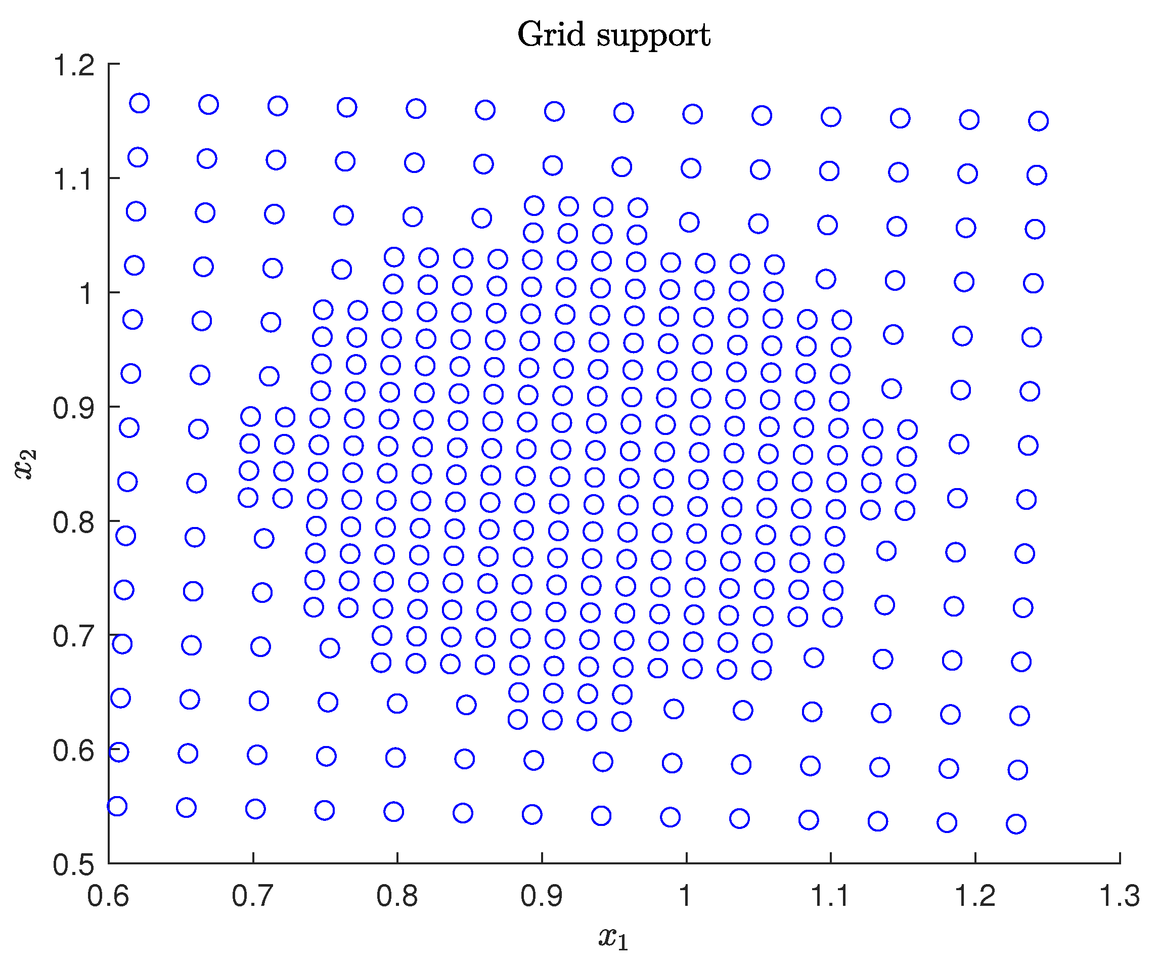
The DDG design is given by the three steps realized by Algorithms 2–4. An example of the final DDG for the PMD shown in Figure 3 can be found in Figure 5.
Compared to the recently proposed DSG, the DDG dense (inner) grid need not be rectangular and, thus, it more realistically covers the support of the conditional PDF with the significant volume without any requirement on computation and utilization of a set of higher-order moments. The DDG design also reduces the user interaction and minimizes the number of the user-defined parameters (compared to the standard grid design, the DDG design requires specification of three additional parameters only; the number of sparse grid points N sparse and the threshold p thr in Algorithm 2 and splitting ration r in Algorithm 4). On the other, the DDG design is slightly more computationally intensive as illustrated in the following section.
5. Numerical Illustration

The influence of the grid design is illustrated in two examples; static point-mass approximation and dynamic state estimation using a PMF with three different grid designs:

5.1. PDF Point-Mass Approximation Quality

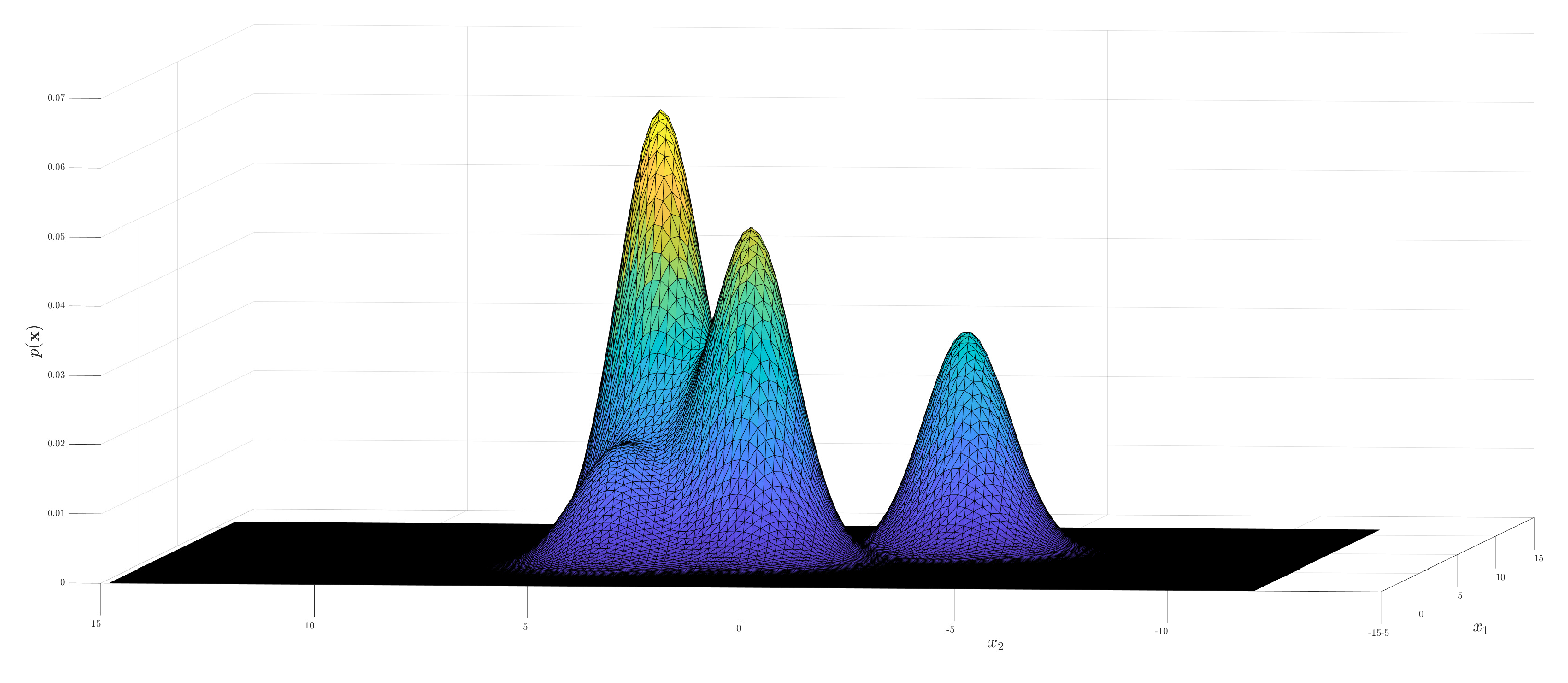
In the first example, let a true two-dimensional, i.e., n x = 2 , Gaussian mixture PDF with four components
p ( x ) = g = 1 4 ω g N { x ; x ^ g , P g }
be considered, where the particular weights, means, and covariance matrices are given as follows
[ ω 1 ω 2 ω 3 ω 4 ] = [ 0.1 0.3 0.4 0.2 ] ,
[ x ^ 1 x ^ 2 x ^ 3 x ^ 4 ] = [ 1 2 4 5 4 1 3.5 3.5 ] ,
P 1 = P 2 = P 3 = P 4 = [ 1 0 0 1 ] .
The PDF is illustrated in Figure 6. The PDF (23) is approximated by the PMD p ^ ( x ; ξ ) (6) with the number of grid points N = { 50 , 200 , 500 } for all three considered grid designs with R covering three STDs. The DSG and DDG designs used such user-defined parameters, which provided the best performance, namely the PMD with the DSG used R i n covering two STDs and the PMD with the DDG used parameters r = 2 and N sparse = 0.4 N .
The quality of the PMD is evaluated using the criteria
  • Integral sum error: ISE = 1 p ^ ( x ; ξ ) d x ,
  • Mean error: ME = i = 1 n x | x ( i ) x ^ PMD ( i ) | .
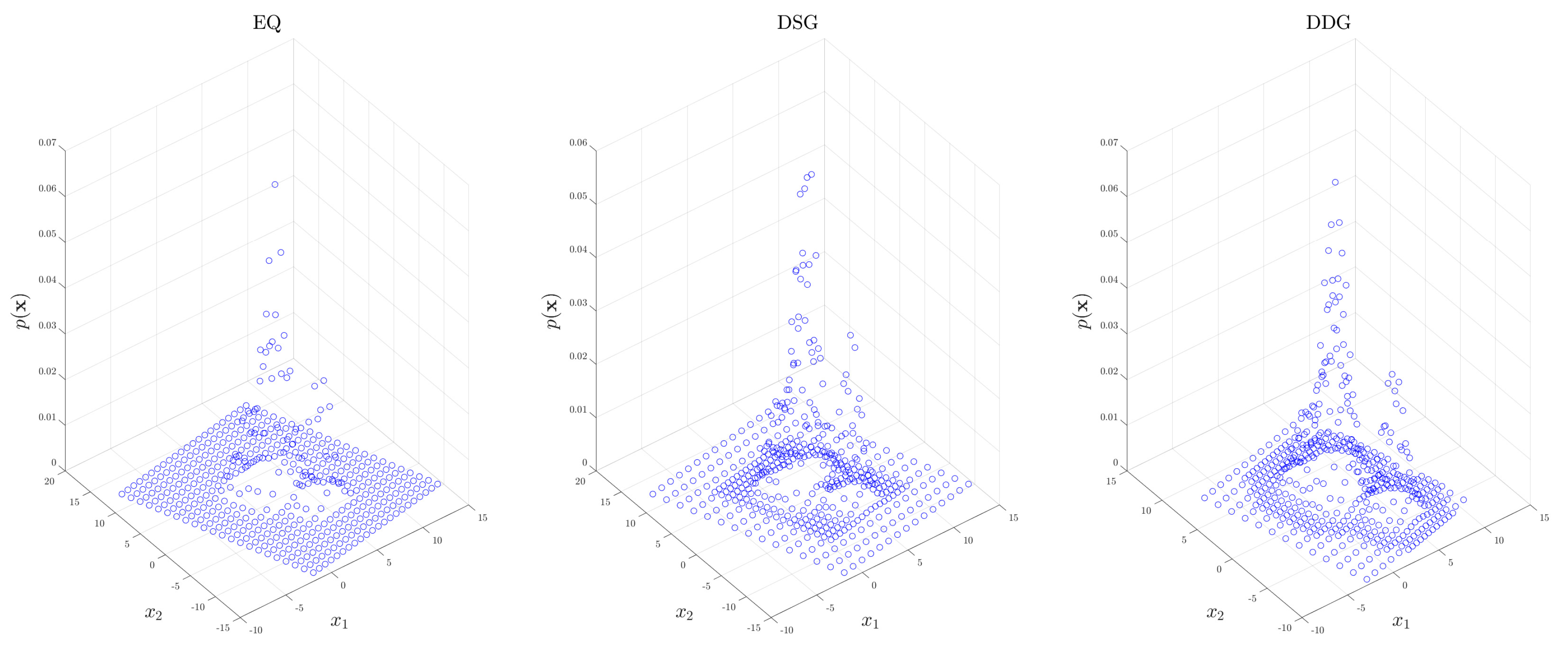
The results can be found in Table 1. It can be seen that the proposed DDG provides the best approximation quality among the considered grids with the same number of points. A degraded performance of the DSG-based design for the approximation of multimodal distributions can also be noted.
For the sake of completeness, a layout of the tested grids is shown in Figure 7.

5.2. PMF in Terrain-Aided Navigation with Spherical Coordinates

The second example considers the terrain-aided navigation (TAN) scenario. The TAN system is a navigation system suitable for GNSS-denied environments, where the vehicle horizontal position is determined by the correlation of the measured vertical terrain profile and the pre-recorded terrain map [23]. The models used in the TAN are highly nonlinear, thus, they are often used as benchmark examples for illustration of the state estimation techniques performance. In this section, the considered the TAN scenario is described by the state-space model [34]
x k + 1 = [ ϕ k + 1 λ k + 1 ] = [ ϕ k + ( φ ( λ k + 1 ) φ ( λ k ) ) tan ( K ) λ k + Δ T V 2 R ( λ k ) cos ( K ) ] + w k ,
z k = h k ( x k ) + v k ,
where k = 0 , 1 , 2 , , 10 , ϕ k is the sought vehicle latitude in degrees, λ k is the longitude in degrees, φ ( λ k ) = log ( 1 + sin ( λ k ) cos ( λ k ) ) , Δ T = 1 is the sampling period in minutes, K = 0.4363 is the constant heading relative to the north in radians (measurement provided e.g., by the compass), V = [ V north , V east ] T is the known constant velocity vector (measurement provided e.g., by an inertial navigation system) in meters/sec, and
R ( λ k ) = ( r 1 2 cos ( λ k ) ) 2 + ( r 2 2 sin ( λ k ) ) 2 ( r 1 cos ( λ k ) ) 2 + ( r 2 sin ( λ k ) ) 2
is Earth radius at latitude λ k . Constants r 1 = 6 , 378 , 137 and r 2 = 6 , 356 , 800 are radii of the Earth at the equator and pole, respectively, in meters. The measurement function h k ( · ) is the the map in the Geographic coordinate system. For the simulation, the maps provided by the Shuttle Radar Topography Mission (SRTM) were used (https://www2.jpl.nasa.gov/srtm/). The noises w k and v k are described as
p ( w k ) = N { w k ; [ 0 0 ] , [ 1.8 · 10 5 0 0 1.8 · 10 5 ] } ,
p ( v k ) = N { v k ; 0 , 3 } .
The PMF was configured with three grid designs with N = 100 , all with R covering ± 4 STDs in each axis (i.e., in latitude and longitude). Namely, the following implementations were compared
  • PMF with equidistant (EQ) grid design,
  • PMF with DSG grid design, where the inner denser grid covers R i n with ± 1 STD in each axis,
  • PMF with the proposed DDG design with the user-defined parameters p thr = 10 4 , N sparse = 50 and r = 3 . Thus, six sparse points with the highest rating d k + 1 ( j ) (22) were split into r 2 × 6 = 54 dense grid points (each sparse point were split into nine dense points). In total, this implementation used N = 44 + 54 = 98 grid points.
Performance of the filters were compared using the following criteria
  • Root-mean-square deviation [ d e g ]: RMSE = i = 1 n x ( x k ( i ) x ^ PMD , k | k ( i ) ) 2 ,
  • Average standard deviation [ d e g ]: ASTD = 1 n x ( diag ( P PMD , k | k ) ) ,
  • time [ s e c ],
in M = 100 Monte–Carlo simulations, where the notation ( A ) is the trace of the matrix A and diag ( A ) stands for the diagonalization of the matrix A , i.e., it zeroes all non-diagonal elements. The results averaged over the time are given in Table 2. It can be seen that the DDG method is better than the equidistant and DSG grid methods, while keeping similar computational complexity. The PMF estimate with the DDG is approximately about 11% more accurate. Note that transformation of the angular longitude and latitude error into the Cartesian coordinate system results in the improvement of the several meters (only by better selection of the grid points and with almost the same computational complexity).

6. Concluding Remarks

The paper focused on the point-mass filter for the nonlinear state estimation with the stress on the grid design as a key filter design step. In particular, a new density difference grid design was proposed. The proposed design was based on evaluation of the predictive PDF in a set of the spare grid points. Subsequently, such point-mass density was differentiated and the state-space regions with significantly varying density were located. These regions are, finally, covered by the dense grid and the detailed point-mass density was completed. The density difference grid properties were analyzed, discussed, and illustrated. It was shown that the point-mass density and the point-mass filter with the proposed grid provides consistently better performance independently of the conditional probability density function shape (e.g., multimodal, heavy-tailed) than with other grid design strategies, while the computational complexity is preserved. The performance was illustrated in two examples, including terrain-aided navigation inspired scenario.

Author Contributions

Conceptualization: J.D., J.M.; Methodology: J.D., O.S.; Investigation: J.M., J.D.; Software: J.M.; Validation: O.S., J.D.; writing: J.D.; J.M., O.S. All authors have read and agreed to the published version of the manuscript.

Funding

This work was supported by the Czech Science Foundation (GACR) under grant GA 20-06054J.

Conflicts of Interest

The authors declare no conflict of interest.

Abbreviations

The following abbreviations are used in this manuscript:
ASTDAverage STD
BRRsBayesian recursive relations
DDGDensity difference grid
DSGDensity specific grid
KFKalman filter
PDFProbability density function
PFParticle filter
PMDPoint-mass density
PMFPoint-mass filter
RMSERoot mean square error
STDStandard deviation

Appendix A. PMF Derivation

The PMF design is based on the numerical solution to the BRRs (3), (4) assuming the PMD form (6) of the conditional PDF. Below, the PMF design is briefly reviewed and a relation to the particle filter is provided. Further details can be found e.g., in [22,26].

Appendix A.1. Initialization

The estimation recursion starts by definition of the initial PDF p ( x 0 | z 1 ) in the form of the PMD p ^ ( x 0 | z 1 ; ξ 0 ) (6) and setting k = 0 .

Appendix A.2. Derivation of Measurement-Update

Derivation of a PMF measurement-update starts with the Bayes’ rule (3) for the posterior density computation, which can be written as
p ( x k | z k ) = c ˜ k 1 p ( z k | x k ) p ( x k | z k 1 ) ,
where p ( x k | z k 1 ) is the predictive density from the last step or from initialization, c ˜ k is a normalization constant and
p ( z k | x k ) = p v k ( z k h k ( x k ) )
is the PDF of a measurement, which is given by (2).
However, only the point-mass approximation of the predictive PDF p ( x k | z k 1 ) is known, i.e., the PMD
p ^ ( x k | z k 1 ; ξ k ) = i = 1 N P k | k 1 ( ξ k ( i ) ) S { x k : ξ k ( i ) , Δ k } .
Substitution of the predictive PMD (A3) into (A1) can be further treated
p ^ ( x k | z k ; ξ k ) c ˜ ^ k 1 p ( z k | x k ) i = 1 N P k | k 1 ( ξ k ( i ) ) S { x k : ξ k ( i ) , Δ k } i = 1 N c ˜ ^ k 1 p ( z k | x k = ξ k ( i ) ) P k | k 1 ( ξ k ( i ) ) P k | k 1 ( ξ k ( i ) ) S { x k : ξ k ( i ) , Δ k } = i = 1 N P k | k ( ξ k ( i ) ) S { x k : ξ k ( i ) , Δ k } ,
where the evaluation of the filtering PDF at ξ k ( i ) is
P k | k ( ξ k ( i ) ) = c ˜ ^ k 1 p ( z k | x k = ξ k ( i ) ) P k | k 1 ( ξ k ( i ) ) .
and the (point-mass) approximate normalization constant is
c ˜ ^ k = i = 1 N P k | k ( ξ k ( i ) ) S { x k : ξ k ( i ) , Δ k } d x k = i = 1 N P k | k ( ξ k ( i ) ) S { x k : ξ k ( i ) , Δ k } d x k = i = 1 N P k | k ( ξ k ( i ) ) δ k .
Note that the support grid stays the same during measurement-update.

Appendix A.3. Derivation of Time-Update

Predictive probability is given by the Chapman–Kolmogorov Equation (4), where p ( x k | z k ) is the filtration density and
p ( x k + 1 | x k ) = p w k ( x k + 1 f k ( x k ) )
is a transition PDF of the state, which is given by the dynamics (1). However, only the approximate filtering PMD (A4) is known and its substitution into (4) reads
p ^ ( x k + 1 | z k ; ξ k ) = p ( x k + 1 | x k ) i = 1 N P k | k ( ξ k ( i ) ) S { x k : ξ k ( i ) , Δ k } d x k .
In order to solve this relation in accord to the PMF design philosophy, a new grid { ξ k + 1 ( j ) } j = 1 N is defined. This grid should cover the part of the state-space where the predictive probability is expected to be. The location and properties of the new grid can be found on the basis of the moment-based prediction as discussed in Section 3.3 or in [22,24]. Having the new grid, i.e., the grid for the time instant k + 1 , the transition PDF (A7) can be approximated by the PMD as follows
p ^ ( x k + 1 | x k ; ξ k + 1 ) = j = 1 N p ( ξ k + 1 ( j ) | x k ) S { x k + 1 : ξ k + 1 ( j ) , Δ k + 1 } .
By substitution of (A9) into (A8), the predictive PMD is of the form
p ^ ( x k + 1 | z k ) p ^ ( x k + 1 | x k ) i = 1 N P k | k ( ξ k ( i ) ) S { x k : ξ k ( i ) , Δ k } d x k = j = 1 N p ( ξ k + 1 ( j ) | x k ) S { x k + 1 : ξ k + 1 ( j ) , Δ k + 1 } i = 1 N P k | k ( ξ k ( i ) ) S { x k : ξ k ( i ) , Δ k } d x k j = 1 N i = 1 N P k | k ( ξ k ( i ) ) p ( ξ k + 1 ( j ) | x k = ξ k ( i ) ) S { x k : ξ k ( i ) , Δ k } S { x k + 1 : ξ k + 1 ( j ) , Δ k + 1 } d x k = i = 1 N j = 1 N P k | k ( ξ k ( i ) ) p ( ξ k + 1 ( j ) | x k = ξ k ( i ) ) S { x k + 1 : ξ k + 1 ( j ) , Δ k + 1 } S { x k : ξ k ( i ) , Δ k } d x k δ k = j = 1 N i = 1 N P k | k ( ξ k ( i ) ) p ( ξ k + 1 ( j ) | x k = ξ k ( i ) ) δ k P k + 1 | k ( ξ k + 1 ( j ) ) S { x k + 1 : ξ k + 1 ( j ) , Δ k + 1 } = j = 1 N P k + 1 | k ( ξ k + 1 ( j ) ) S { x k + 1 : ξ k + 1 ( j ) , Δ k + 1 } ,
where the predictive probability value at a new grid point ξ k + 1 ( j ) is
P k + 1 | k ( ξ k + 1 ( j ) ) = i = 1 N p ( ξ k + 1 ( j ) | x k = ξ k ( i ) ) P k | k ( ξ k ( i ) ) δ k , j .
The expression (A10), commonly denoted as the convolution, is the most computationally demanding step of the PMF. Note that the value of P k + 1 | k ( ξ k + 1 ( j ) ) is independent over j, therefore parallel programming and computing tools can be used to speed the algorithm up.

Appendix A.4. Relation of Point-Mass and Particle Filters

The point-mass filter and particle filter (PF) are based on numerical, i.e., point-based, solution to the BRRs (3), (4). Whereas, the PMF solves the BRRs using the deterministic integration rule, the PF uses the stochastic Monte-Carlo integration techniques [20]. The main difference can be, thus, found in the generation of the points. In the PMF, the points are generated in, possibly equally spaced, grid covering (approximating) a significant part of the state space and the conditional PDF is computed in the grid points only. On the other hand, in the PF, the conditional PDF is approximated by the set of samples, which means, that in parts of the state space with “higher values” of the conditional PDF, a higher number of the samples can be expected. Consequently, the PF does not include the convolution, as the PMF, and, thus, it is computationally cheaper. As an advantage of the PMF over the PF, its deterministic behavior can be mentioned. Contrary to the PMF, the PF may not provide the same estimates while repetitively processing the same data on different platforms. This property may be limiting for certain safety-critical applications [23].

References

  1. Simon, D. Optimal State Estimation: Kalman, H Infinity, and Nonlinear Approaches; Wiley-Interscience: New York, NY, USA, 2004. [Google Scholar]
  2. Abur, A.; Expósito, A. Power System State Estimation: Theory and Implementation; CRC Press: Boca Raton, FL, USA, 2004. [Google Scholar]
  3. Hering, P.; Janeček, P.; Janeček, E. On-line Ampacity Monitoring from Phasor Measurements. In Proceedings of the 19th IFAC World Congress; Elsevier: Cape Town, South Africa, 2014. [Google Scholar]
  4. Guo, P.; Infield, D. Wind Turbine Tower Vibration Modeling and Monitoring by the Nonlinear State Estimation Technique (NSET). Energies 2012, 7, 5279–5293. [Google Scholar] [CrossRef] [Green Version]
  5. Wang, D.; Guan, X.; Liu, T.; Gu, Y.; Shen, C.; Xu, Z. Ext. Distrib. State Estim. A Detect. Method Tolerable False Data Inject. Attacks Smart Grids. Energies 2014, 7, 1517–1538. [Google Scholar] [CrossRef] [Green Version]
  6. Antončič, M.; Papič, I.; Blažič, B. Robust Fast State Estim. Poorly-Obs. Low Volt. Distrib. Networks Based Kalman Filter Algorithm. Energies 2019, 7, 4457. [Google Scholar] [CrossRef] [Green Version]
  7. Yu, Z.; Huai, R.; Xiao, L. State- Estim. Lithium-Ion Batter. Using A Kalman Filter Based Local Linearization. Energies 2015, 8, 7854–7873. [Google Scholar] [CrossRef] [Green Version]
  8. Zhang, R.; Xia, B.; Li, B.; Cao, L.; Lai, Y.; Zheng, W.; Wang, H.; Wang, W. State Art Lithium-Ion Battery SOC Estim. Electr. Veh. Energies 2018, 11, 1820. [Google Scholar] [CrossRef] [Green Version]
  9. Simon, D. Adaptive Filtering and Change Detection; John Wiley & Sons: Hoboken, NJ, USA, 2000. [Google Scholar]
  10. Lindfors, M.; Hendeby, G.; Gustafsson, F.; Karlsson, R. Vehicle Speed Tracking Using Chassis Vibrations. In Proceedings of the 2016 IEEE Intelligent Vehicles Symposium, Gothenburg, Sweden, 19–22 June 2016. [Google Scholar]
  11. Bar-Shalom, Y.; Li, X.R.; Kirubarajan, T. Estimation with Applications to Tracking and Navigation: Theory Algorithms and Software; John Wiley & Sons: Hoboken, NJ, USA, 2001. [Google Scholar]
  12. Groves, P.D. Principles of GNSS, Inertial, and Multisensor Integrated Navigation Systems; Artech House: Norwood, MA, USA, 2008. [Google Scholar]
  13. Sorenson, H.W. On the Development of Practical Nonlinear Filters. Inf. Sci. 1974, 7, 230–270. [Google Scholar] [CrossRef]
  14. Šimandl, M.; Duník, J. Derivative-free Estimation Methods: New Results and Performance Analysis. Automatica 2009, 45, 1749–1757. [Google Scholar] [CrossRef]
  15. Anderson, B.D.O.; Moore, J.B. Optimal Filtering; Prentice Hall: Englewood Cliffs, NJ, USA, 1979. [Google Scholar]
  16. Julier, S.J.; Uhlmann, J.K. Unscented Filtering and Nonlinear Estimation. IEEE Proc. 2004, 92, 401–421. [Google Scholar] [CrossRef] [Green Version]
  17. Duník, J.; Straka, O.; Šimandl, M. Stochastic Integration Filter. IEEE Trans. Autom. Control 2013, 58, 1561–1566. [Google Scholar] [CrossRef]
  18. Särkkä, S. Bayesian Filtering and Smoothing; Cambridge University Press: Cambridge, UK, 2013. [Google Scholar]
  19. Sorenson, H.W.; Alspach, D.L. Recursive Bayesian Estimation Using Gaussian Sums. Automatica 1971, 7, 465–479. [Google Scholar] [CrossRef]
  20. Doucet, A.; De Freitas, N.; Gordon, N. (Eds.) Sequential Monte Carlo Methods in Practice; Springer: Berlin/Heidelberg, Germany, 2001. [Google Scholar]
  21. Šimandl, M.; Královec, J.; Söderström, T. Anticipative Grid Design in Point-Mass Approach to Nonlinear State Estimation. IEEE Trans. Autom. Control 2002, 47, 699–702. [Google Scholar] [CrossRef]
  22. Bergman, N. Recursive Bayesian Estimation: Navigation and Tracking Applications. Ph.D. Thesis, Linköping University, Linköping, Sweden, 1999. [Google Scholar]
  23. Duník, J.; Soták, M.; Veselý, M.; Straka, O.; Hawkinson, W.J. Design of Rao-Blackwellised Point-Mass Filter with Application in Terrain Aided Navigation. IEEE Trans. Aerosp. Electron. Syst. 2019, 55, 251–272. [Google Scholar] [CrossRef]
  24. Matoušek, J.; Duník, J.; Straka, O. Point-Mass Filter: Density Specific Grid Design and Implementation. In Proceedings of the 15th European Workshop on Advanced Control and Diagnosis, Bologna, Italy, 21–22 November 2019. [Google Scholar]
  25. Šmídl, V.; Gašperin, M. Rao-Blackwellized Point Mass Filter for Reliable State Estimation. In Proceedings of the 16th International Conference on Information Fusion, Istanbul, Turkey, 9–12 July 2013. [Google Scholar]
  26. Šimandl, M.; Královec, J.; Söderström, T. Advanced Point-mass Method for Nonlinear State Estimation. Automatica 2006, 42, 1133–1145. [Google Scholar] [CrossRef]
  27. Sirola, N. Nonlinear Filtering with Piecewise Probability Densities. Ph.D. Thesis, Tampere University of Technology, Tampere, Finland, 2007. [Google Scholar]
  28. Yoo, Y.M.; Park, C.G. Improvement of Terrain Referenced Navigation using a Point Mass Filter with Grid Adaptation. Int. J. Control. Autom. Syst. 2015, 13, 1173–1181. [Google Scholar] [CrossRef]
  29. Peng, D.; Zhou, T.; Xu, C.; Zhang, W.; Shen, J. Marginalized Point Mass Filter with Estimating Tidal Depth Bias for Underwater Terrain-Aided Navigation. J. Sens. 2019, 2019. [Google Scholar] [CrossRef]
  30. Bergman, N. Bayesian Approach to Terrain-Aided Navigation. In 11th IFAC Symposium on System Identification; Elsevier: Kitakyushu/Fukuoka, Japan, 1997; pp. 1531–1536. [Google Scholar]
  31. Jeon, H.C.; Park, W.J.; Park, C.G. Grid Design for Efficient and Accurate Point Mass Filter-Based Terrain Referenced Navigation. IEEE Sens. J. 2018, 18, 1731–1737. [Google Scholar] [CrossRef]
  32. Duník, J.; Straka, O.; Šimandl, M.; Blasch, E. Random-Point-Based Filters: Analysis and Comparison in Target Tracking. IEEE Trans. Aerosp. Electron. Syst. 2015, 51, 303–308. [Google Scholar] [CrossRef]
  33. Nørgaard, M.; Poulsen, N.K.; Ravn, O. New Developments in State Estimation for Nonlinear Systems. Automatica 2000, 36, 1627–1638. [Google Scholar] [CrossRef]
  34. Musso, C.; Bresson, A.; Bidel, Y.; Zahzam, N.; Dahia, K.; Allard, J.; Sacleux, B. Absolute Gravimeter for Terrain-aided Navigation. In Proceedings of the 20th International Conference on Information Fusion, Xi’an, China, 10–13 July 2017. [Google Scholar]
Figure 1. Illustration of point-mass probability density function (PDF) approximation (grid points—red; grid point neighbourhood—blue; scaled selection function—green).
Energies 13 04080 g001
Figure 2. Illustration of search for sparse grid boundaries.
Energies 13 04080 g002
Figure 3. Illustration of sparse points difference ratings.
Energies 13 04080 g003
Figure 4. Illustration of splitting for the ratio r = 2 .
Energies 13 04080 g004
Figure 5. Example of grid support.
Energies 13 04080 g005
Figure 6. Static example: illustration of Gaussian mixture PDF.
Energies 13 04080 g006
Figure 7. Static example: grids with 500 grid points.
Energies 13 04080 g007
Table 1. Approximation errors of the point-mass density (PMD) with three different grid designs.
N50200500
EQISE0.04680.0062 5.5585 × 10 8
ME1.5848 0.0606 2.4479 × 10 5
DSGISE0.0733 6.3488 × 10 5 3.8642 × 10 5
ME0.7567 6.1405 × 10 5 3.1102 × 10 4
DDGISE 1.1102 × 10 15 2.2204 × 10 16 2.2204 × 10 16
ME0.2439 2.5314 × 10 5 6.7043 × 10 6
Table 2. Estimation results.
EQDSGDDG
RMSE [ d e g ] 0.0156750.0155210.013853
ASTD [ d e g ] 0.0127410.0124660.012999
Time [ s e c ] 0.260610.261310.26656