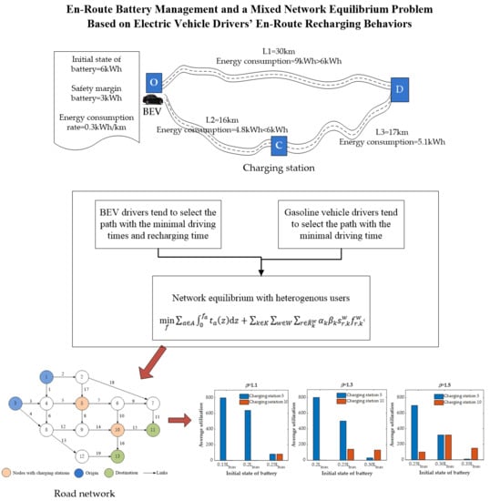
En-Route Battery Management and a Mixed Network Equilibrium Problem Based on Electric Vehicle Drivers’ En-Route Recharging Behaviors

Abstract

With the rapidly increasing number of electric vehicle users, in many urbans transport networks, there are mixed traffic flows (i.e., electric vehicles and gasoline vehicles). However, limited by driving ranges and long battery recharging, the battery electric vehicle (BEV) drivers’ route choice behaviors are inevitably affected. This paper assumes that in a transportation network, when BEV drivers are traveling between their original location and destinations, they tend to select the path with the minimal driving times and recharging time, and ensure that the remaining charge is not less than their battery safety margin. In contrast, gasoline vehicle drivers tend to select the path with the minimal driving time. Thus, by considering BEV drivers’ battery management strategies, e.g., battery safety margins and en-route recharging behaviors, this paper developed a mixed user equilibrium model to describe the resulting network equilibrium flow distributions. Finally, a numerical example is presented to demonstrate the mixed user equilibrium model. The results show that BEV drivers’ en-route recharging choice behaviors are significantly influenced by their battery safety margins, and under the equilibrium, the travel routes selected by some BEV drivers may not be optimal, but the total travel time may be more optimal.

1. Introduction

Thanks to the rapid development of battery technologies and increasing price of crude oil [1,2,3,4], in recently years, the number of battery electric vehicles (BEVs) is increasing rapidly in many cities in the world. However, for many BEV users, although the number of charging stations is increasing in the urban area, they still fear that their vehicle may run out of power when driving between their original location and destination. This fear, known as range anxiety [5,6,7], is not only experienced by BEV drivers, but also by alternative-fuel vehicles drivers [8,9]. Nevertheless, for alternative-fuel vehicle drivers, range anxiety can be easily eliminated by taking onboard spare fuel cans. However, for BEV drivers, it seems unrealistic to take onboard spare batteries for replacing. Furthermore, to ease range anxiety, many BEV drivers are likely to set a battery safety margin to ensure the remaining battery can finish the trip [10,11,12]. Moreover, range anxiety also makes some BEV drivers prefer the path on which they can easily access charging stations. In a word, range anxiety will inevitably affect BEV drivers’ travel choice behaviors. Thus, in the future, with BEVs widely participating in urban transportation, the equilibrium distribution of the urban traffic flow will be influenced.

However, in the research of traffic assignment, the assumptions of travelers’ choice behaviors play an important role in solving network equilibrium problems [13,14,15,16,17]. Thus, in order to understand how BEVs influence the equilibrium distribution of the urban traffic flow, the assumptions of BEV drivers’ travel choice behaviors and the assumptions of BEVs’ structure and characteristics will be important. For example, by considering electric vehicles’ limited driving range and drivers’ recharging behaviors, He et al. [18] proposed a network equilibrium model. In their research, they assumed that there are only BEVs in the network and these BEVs are homogeneous with the same battery size and same initial state of battery, and that BEV drivers are rational. These assumptions are restrictive and may lead a discrepancy between the research results and reality. Then, by considering stochastic range anxiety, Xie et al. [19] developed a network equilibrium with electric vehicles. In their research, they assumed that the variation of driving distance limits BEV drivers’ perception and causes battery depletion of BEV drivers with heterogeneous perception errors and risk-taking behaviors. In addition, Jiang and Xie [20] and Xu et al. [21] considered a mixed network equilibrium problem with two vehicle types, i.e., gasoline vehicles and electric vehicles. In the former, a path-constrained traffic assignment is formulated; in the latter, a nonlinear minimization model in terms of path flows is formulated. The above studies lack of consideration on BEV drivers’ recharging psychological barriers.

Becker [22] suggested that the utility of time spent at a meaningful activity is larger than the utility of time spent at a non-meaningful activity. Since recharging activity is an additional activity and makes BEV drivers’ total travel time become longer, for BEV drivers who need to rechange their BEVs at en-route charging stations, their perception of disutility of unit driving time may be different from their perception of disutility of unit recharging time. Thus, to be more in line with reality, in this paper, we assume that there are two kinds of vehicles in the network, i.e., gasoline vehicles and electric vehicles; moreover, BEV energy consumption is not influenced by traffic congestion and is independent of traffic flows [5,23,24]. Then, for battery electric vehicles, assuming that these BEVs have the same battery size but different initial state of battery, and for BEV drivers who need recharging en-route, it is assumed that they are heterogenous with different risk attitudes (this can be reflected by different battery safety margins) and that their perceptions of disutility of unit recharging time is smaller than the perception of disutility of unit travel time. That is, if the value of the travel time coefficient is equal to the value of the recharging time coefficient, there must be an error in some BEV drivers’ minimal recharging time perception that makes their actual minimal recharging time longer. Based on the above assumptions and considering BEV drivers’ range anxiety and recharging behavior, we formulate a mixed network equilibrium model to deal with the traffic assignment of gasoline vehicles and electric vehicles.

In summary, the contribution of this paper is that by considering different types of drivers with different risk attitudes, different perception errors, and different initial states of battery, we developed a mixed user equilibrium model to describe gasoline vehicle drivers’ route choice behavior, BEV drivers’ en-route recharging behaviors, the utilization of charge stations, and the distribution of traffic flow in the network under a long-term equilibrium. The results of this paper can help to understand how BEV drivers’ battery management strategies (e.g., battery safety margin setting and en-route recharging behavior) influence urban transport systems.

The remainder of this paper is organized as follows: Section 2 formulates a base model that describes a mixed network equilibrium, and then a solution procedure is proposed. In Section 3, a numerical example is presented, and the numerical example results and some conclusions are also presented. Finally, Section 4 concludes the paper.

2. Base Model

2.1. The Characterization of a Traffic Network

Let $G=\left(N,A\right)$ denote a traffic network where $N$ is set of nodes and $A$ is set of links. Let $W$ be the set of origin–destination pairs (hereinafter referred to as “OD pairs”) and $w\in W$ be the OD pair index. Let $R_w$ and $D_w$ be the set of paths and the travel demand between OD pair $w$, and $r\in R_w$ the path index. We denote a link as $a\in A$, and $f_a$ is the corresponding link flow. Let ${\delta }_{a,r}^w$ be the path-link incidence. If path $r$ traverses link $\mathrm{a}$, then ${\delta }_{a,r}^w=1$, otherwise ${\delta }_{a,r}^w=0$. Let $f_a$ be the traffic flow on link $a$ and $z_a$be the travel distance of link $a$. The travel time of link $a$ is a strictly increasing function of the flow in the link, for example, in this study, we used the following Bureau of Public Roads (BPR) function:

$$t_a=t_a^0\left[1+0.15{\left(\frac{f_a}{c_a}\right)}^4\right]$$

(1)

where $t_a^0$ is link $a$’s free-flow travel time, and $c_a$ is link $a$’s capacity.

2.2. Definition and Formulation of a Mixed User Equilibrium

In this paper, it is assumed that there are two kinds of vehicle drivers in the network, i.e., BEV drivers and gasoline vehicle drivers. For BEV drivers, they many need rechange their BEVs at one en-route charging station to avoid running out of charge before reaching their destinations. It is worth mentioning that this paper assumes that in order to reach the destination as quickly as possible, the BEVs will not be fully charged at the en-route charging station; BEV drivers will recharge a small amount of electricity (this also suggests that the values of travel time are higher for these BEV drivers). In addition, due to the uncertainty of fuel consumption, BEV drivers may avoid using all of the power supplied by their batteries when they arrive at the destinations. Instead, they prefer to set a battery safety margin that they keep the remaining battery higher than [10]. Thus, we assumed that when BEV drivers arrive their destinations, the remaining battery is no less than the battery safety margin. This battery safety margin will ensure that they can find the next charging station to keep the BEV going. Note that in this paper, the minimal recharging amount of electricity depends on the remaining distance traveled and BEV drivers’ battery safety margins. Figure 1 is an example used to illustrate the en-route recharging behavior. As shown in Figure 1, the BEV’s initial state of battery is 6 kWh, the energy consumption rate is 0.3 kWh/km [18], and the BEV driver’s battery safety margin is 3 kWh. Then, under this setting, this BEV driver will choose path 2 and the amount of recharging electricity will be 6.9 kWh. On the other hand, for gasoline vehicle drivers, it is assumed that they have enough fuel.

When traveling between their original location and destination, for each driver, it is assumed that they select the route with minimal travel costs, which includes the cost of travel time and electricity. It is worth mentioning that the cost of travel time is much higher than the cost of electricity [25]. Thus, we only consider travel time cost when drivers select paths. Notably, for BEV drivers who need recharging en-route, their total travel time includes driving time and recharging time. Moreover, different from others’ research, in our based model, we consider heterogenous BEV drivers with different risk attitudes and different levels of perception errors regarding the values of recharging time, and the BEVs have the same battery size but a different initial state of battery. Moreover, we further assumed that in the transport network, there is only a finite number of charging stations, and these charging stations are located at certain nodes of the network. Note that a vehicle traveling along a path may not pass by a charging station. Thus, based on the above assumptions and considerations, we can obtain the following network equilibrium:

Definition 1.

In a long-term equilibrium, for the same type of drivers, all the utilized paths are usable and the total travel time costs of all the utilized paths of one OD pair are the same, that is, they are less than or equal to those of any unutilized usable paths of the same OD pair.

Here, a mathematic model will be proposed to describe the above long-term equilibrium. For convenience, it is assumed that there are $K$ types of vehicle drivers in the network where $K-1$ types belong to BEV drivers and they have different risk attitudes and different levels of perception of rechanging time. The remaining type belongs to gasoline vehicle drivers. Moreover, because BEV energy consumption is independent of traffic flow, let ${\widehat{R}}_w$ denote the set of all usable paths between OD pair $w$, thus, we can obtain following network equilibrium with heterogenous users (NE-HU):

$$\mathrm{NE}-\mathrm{HU}: \underset{f}{\min }{{\displaystyle \sum }}_{a\in A}{{\displaystyle \int }}_0^{f_a}{t}_a\left(z\right)\mathrm{d}z+{{\displaystyle \sum }}_{k\in K}{{\displaystyle \sum }}_{w\in W}{{\displaystyle \sum }}_{r\in {\widehat{R}}_k^w}{\alpha }_k{\beta }_k{s}_{r,k}^w{f}_{r,k}^w$$

(2)

$$\mathrm{s}.\mathrm{t}. {{\displaystyle \sum }}_{r\in R_w}{f}_r^w=D_w \forall w\in W$$

(3)

$${{\displaystyle \sum }}_{k\in K}{\displaystyle \sum }_{r\in {\widehat{R}}_k^w}{f}_{r,k}^w=g_k^w \forall w\in W,k\in K$$

(4)

$$f_{r,k}^w\ge 0 \forall r\in {\widehat{R}}_k^w,w\in W,k\in K$$

(5)

$$f_a={{\displaystyle \sum }}_{k\in K}{{\displaystyle \sum }}_{w\in W}{{\displaystyle \sum }}_{r\in {\widehat{R}}_k^w}{f}_{r,k}^w{\delta }_{a,r}^w \forall a\in A,k\in K$$

(6)

where, $s_{r,k}^w$ is the minimal actual time (minutes) that drivers need to spend on recharging activity. Moreover, for gasoline vehicle drivers, there is $s_{r,k}^w$ = 0. ${\beta }_k\left(\ge 1\right)$ is a coefficient and relates to the drivers’ risk attitudes. ${\alpha }_k\left(\ge 1\right)$is a coefficient and relates to BEV drivers’ perception errors of the values of recharging time. Note that limited by cognitive ability, drivers may not be able to accurately estimate their recharging times, thus, the “perception error” in this study is defined as the difference between a BEV driver’s perceived value of recharging time and the actual value of recharging time. Moreover, ${\alpha }_k$ = 1 indicates that a driver’s perception of disutility of unit travel time is equal to their perception of disutility of unit recharging time, and the greater the value of ${\alpha }_k$, the smaller the perception of disutility of unit recharging time. $g_k^w$ is travel demand (i.e., total vehicles) of type $k$ between OD pair $w$, and $f_{r,k}^w$ (veh/h) is the traffic flow of type $k\in K$ on path $r$ between OD pair $w$.

Then, the above NE-HU model’s Karush-Kuhn-Tucker (KKT) conditions can be written as:

$${\displaystyle \sum }_a{t}_a\left(f_a\right)\frac{\partial f_a}{\partial f_{a,k}^w}+{\alpha }_k{\beta }_k{s}_r^w-{\lambda }_k^w-{\mu }_{k,r}^w=0$$

(7)

$${\displaystyle \sum }_{r\in {\widehat{R}}_k^w}{f}_{r,k}^w=g_k^w$$

(8)

$$f_{r,k}^w\ge 0$$

(9)

$${\mathsf{\mu }}_{\mathrm{k},\mathrm{r}}^{\mathrm{w}}\ge 0$$

(10)

$$f_{r,k}^w·{\mu }_{k,r}^w=0$$

(11)

where $\frac{\partial f_a}{\partial f_{a,k}^w}={\delta }_{a,r}^w$ and ${\displaystyle \sum }_a{t}_a\left(f_a\right){\delta }_{a,r}^w=t_r^w$. Moreover, $t_r^w$ is the travel time (minutes) of path $r$. Thus, Equation (7) can be further written as:

$${\mu }_{k,r}^w=t_r^w+{\alpha }_k{\beta }_k{s}_r^w-{\lambda }_k^w$$

(12)

Finally, based on the Equations (10)–(12), we can obtain the following conditions:

$$t_r^w+{\alpha }_k{\beta }_k{s}_r^w-{\lambda }_k^w\ge 0$$

(13)

$$f_{r,k}^w·\left(t_r^w+{\alpha }_k{\beta }_k{s}_r^w-{\lambda }_k^w\right)=0$$

(14)

Here, Equation (14) is a complementary condition. When $r\in {\widehat{R}}_k^w$, if $f_{r,k}^w=0$, then $t_r^w+{\alpha }_k{\beta }_k{s}_r^w\ge {\lambda }_k^w$; if $f_{r,k}^w\ge 0$, then $t_r^w+{\alpha }_k{\beta }_k{s}_r^w-{\lambda }_k^w=0$. However, when $r\notin {\widehat{R}}_k^w$, $f_{r,k}^w=0$. This complementary condition guarantees that the traffic flow is only distributed on the usable paths.

2.3. Solution Procedure

The above NE-HU model is a convex program with linear constraints. We can solve it by the enumeration method. However, the work of enumerating all the usable paths will be tremendous. Thus, in this paper, we adopt an iterative solution procedure which was proposed by He et al. [18]. However, different from He’s work, in this paper, we consider the perception recharging time instead of actual recharging time and heterogenous BEV drivers with the different risk attitudes and different levels of perception of recharging time. Thus, the sub-problem, finding the shortest usable path by considering BEV drivers’ perception of recharging time (SP-PT), can be formulated as follows:

$$\mathrm{SP}-\mathrm{PT}: \underset{x,r,l}{\min }{{\displaystyle \sum }}_{k\in K}{{\displaystyle \sum }}_{a\in A}{t}_a\left({\tilde{f}}_a\right)x_{a,k}^w+{{\displaystyle \sum }}_{k\in K}{{\displaystyle \sum }}_{i\in N}{\alpha }_k\left(c_i^1{y}_{i,k}^w+c_i^2{\beta }_k{l}_{i,k}^w\right)$$

(15)

$$\mathrm{s}.\mathrm{t}. ∆{\mathit{x}}_k^w=E_k^w$$

(16)

$$L_{j,k}^w-L_{i,k}^w+z_a\varpi -{\beta }_k{l}_{j,k}^w={\rho }_{a,k}^w \forall \left(i,j\right)=a\in A$$

(17)

$$L_{i,k}^w-z_a\varpi \ge -M\left(1-x_{a,k}^w\right)+{\beta }_{k}m \forall \left(i,j\right)=a\in A$$

(18)

$$-H\left(1-x_{a,k}^w\right)\le {\rho }_{a,k}^w\le H\left(1-x_{a,k}^w\right) \forall \left(i,j\right)=a\in A$$

(19)

$$0\le L_{i,k}^w\le L_{max} \forall i\in N$$

(20)

$$L_{o\left(w\right),k}^w=L_{0,k} \forall i\in N$$

(21)

$$x_{a,k}^w\in \left\{0,1\right\} \forall \left(i,j\right)\in A$$

(22)

$$y_{i,k}^w\in \left\{0,1\right\} \forall i\in N$$

(23)

where, $l_{i,k}^w$ (kWh) is the recharging amount of electricity in theory at charging stations $i$ for type $k$ drivers, and ${\beta }_k{l}_{i,k}^w$ (kWh) is the actual recharging amount of electricity for type $k$ drivers when considering their different risk attitudes. Let $c_i\left({\beta }_k{l}_{i,k}^w\right)$ represent the recharging time (minutes) that at node $i\in N$, type $k$ drivers spend recharging ${\beta }_k{l}_{i,k}^w$ amount of electricity. Then, ${\alpha }_k{c}_i\left({\beta }_k{l}_{i,k}^w\right)$ is the perception of time for type $k$ drivers to recharge ${\beta }_k{l}_{i,k}^w$ amount of electricity. In this paper, the following perception of charging time function is used, i.e., ${\alpha }_k{c}_i\left({\beta }_k{l}_{i,k}^w\right)={\alpha }_k{c}_i^1+{\alpha }_k{c}_i^2{\beta }_k{l}_{i,k}^w$, and here $c_i^1$ (minutes) represents the fixed recharging time; $c_i^2$ ($\min /\mathrm{kWh}$) is a variable of recharging time and relies on the class of chargers, for example, direct current charging (fast charging) and alternating current charging (slow charging). However, in this study, it is assumed that the en-route charging stations only supply direct current charging facilities and the charging facilities are adequate. Note that if there is no charging station on node $i$, the value of ${\alpha }_k{c}_i\left({\beta }_k{l}_{i,k}^w\right)$ will be zero, and for gasoline vehicle drivers, the value of ${\alpha }_k{c}_i\left({\beta }_k{l}_{i,k}^w\right)$ will also be zero.

Moreover, $L_{j,k}^w$ (kWh) is the battery charge after recharging, $L_{max}$ (kWh) is the battery size, and $L_{0,k}$ (kWh) is the initial state of battery charge. $∆$ is the node-link incidence matrix, $E_k^w$ is a vector with a length of $\left|N\right|$ and consists of two nonzero components: one has a value of 1, which corresponds to the original location; the other has a value of −1 which corresponds to the destination. $x_{a,k}^w$ is a binary variable, and if link $a$ is used, then $x_{a,k}^w=1$, otherwise $x_{a,k}^w=0$; $y_{i,k}^w$ is also a binary variable, and if charging station $i$ is selected, then $y_{i,k}^w=1$, otherwise, $y_{i,k}^w=0$. ${\rho }_{a,k}^w=0$ if link $a$ is used by driver $k$ and unrestriced otherwise. $\varpi$ is the BEV’s energy consumption, $m$ is the minimum comfortable range, and $H$ and $M$ are sufficiently large constants.

In the above SP-PT model, the objective function is to minimize the total trip time, including driving time (i.e., ${\displaystyle \sum }_{k\in K}{\displaystyle \sum }_{a\in A}{t}_a\left({\tilde{f}}_a\right)x_{a,k}^w$) and BEV drivers’ perceived recharging time (i.e., ${\displaystyle \sum }_{k\in K}{\displaystyle \sum }_{i\in N}{\alpha }_k\left(c_i^1{y}_{i,k}^w+c_i^2{\beta }_k{l}_{i,k}^w\right)$. Constraint (16) ensures flow balance. Constraints (17) and (19) specify the relationship between the states of charge of BEV batteries at the starting and ending nodes of any utilized link. Constraint (18) ensures that the BEV driver will not fully deplete their battery on any utilized link, and the BEV driver prefers to keep the remaining battery range no less than a comfortable range.

Let $\left(\dots ,{\tilde{x}}_{a,k}^w,\dots ,{\tilde{y}}_{i,k}^w,\dots ,{\tilde{l}}_{i,k}^w,\dots \right)$ be the optimal solution to SP-PT for OD pair $w\in W$ for each type of $k\in K$. By solving ${\tilde{x}}_{a,k}^w$, we can obtain the shortest usable path, i.e., ${\tilde{r}}_k^w$. Moreover, through solving ${\tilde{y}}_{i,k}^w$ and ${\tilde{l}}_{i,k}^w$, we can obtain the shortest perception recharging time, i.e., ${\displaystyle \sum }_{k\in K}{\displaystyle \sum }_{i\in N}{\alpha }_k\left(c_i^1{y}_{i,k}^w+c_i^2{\beta }_k{l}_{i,k}^w\right)$. Then, to solve NE-HU, we can use the following iterative procedures:

Step 1: For each type of $k\in K$ between OD pair $w\in W$ solve SP-PT, i.e., $\left(\dots , {\tilde{f}}_a, \dots \right)=\left(\dots , 0, \dots \right)$. Obtain the initial usable path set ${\tilde{R}}_k^w=\left\{{\tilde{r}}_k^w\right\}$ and calculate the minimal actual recharging time $s_{\tilde{r},k}^w=c_i^1{y}_{i,k}^w+c_i^2{\beta }_k{l}_{i,k}^w$.

Step 2: Based on the initial usable path set ${\tilde{R}}_k^w=\left\{{\tilde{r}}_k^w\right\}$, solve the NE-HU model and obtain the optimal traffic flow distribution, i.e., $\left(\dots , {\tilde{f}}_{a,\mathrm{k}}, \dots \right)$ and the Lagrange multiplier, i.e., $\left(\dots , {\lambda }_k^w, \dots \right)$.

Step 3: Solve the SP-PT model. For each type of $k\in K$ and each OD pair $w\in W$, if ${\lambda }_k^w\le {\displaystyle \sum }_{k\in K}{\displaystyle \sum }_{a\in A}{t}_a\left({\tilde{f}}_a\right)x_{a,k}^w+{\displaystyle \sum }_{k\in K}{\displaystyle \sum }_{i\in N}{\alpha }_k\left(c_i^1{y}_{i,k}^w+c_i^2{\beta }_k{l}_{i,k}^w\right)$, then stop and $\left(\dots , {\tilde{f}}_{a,\mathrm{k}}, \dots \right)$ is the optimal equilibrium link flow distribution; otherwise, go to Step 1.

3. Numerical Example

To demonstrate the above mixed user equilibrium model, a numerical example will be shown in this section. We considered the following Nguyen–Dupius network [26] (see Figure 2). There are 13 nodes, 19 links, and four OD pairs in the Nguyen–Dupius network. We assume that the link distances are two times the link’s free-flow travel times, and the link characteristics are shown in

Table 1. Link capacity (veh/h), distance (km) and free-flow travel time (min).

Link	Distance	Free-Flow Travel Time	Capacity	Link	Distance	Free-Flow Travel Time	Capacity
1	14	7	3000	11	18	9	5000
2	18	9	2000	12	20	10	5500
3	18	9	2000	13	18	9	2000
4	24	12	2000	14	12	6	4000
5	6	3	3500	15	18	9	3000
6	18	9	4000	16	16	8	3000
7	10	7	5000	17	14	7	2000
8	26	13	2500	18	20	10	5000
9	10	5	2500	19	18	9	2000
10	18	9	2000

. According to the Nissan Leaf 2020 [27], in the numerical example, we set the battery capacity as $L_{max}=40 \mathrm{kWh}$ and the energy consumption rate as $\varpi =0.167 \mathrm{kWh}/\mathrm{km}$. Since in this paper we assume the en-route charging stations only supply direct current charging facilities (fast charging facilities), then the fixed time $c_i^1=5 \min \mathrm{the}$ variable time $c_i^2=0.6 \min /\mathrm{kWh}$ if the current battery level is less than 70%, and $c_i^2=10 \min /\mathrm{kWh}$ if the current battery level is higher than 70%. Note that in this paper, it is assumed that in order to reach the destination as quickly as possible, BEV drivers do not fully charge their electric car at the en-route charging station.

As shown in Figure 2, in the network, the charge stations are located in the nodes 5 and 10. It is assumed that in the network, 30% of vehicle drivers are BEV drivers, and the rest are gasoline vehicle drivers. Because of the different risk attitudes towards en-route recharging, BEV drivers are further divided into three different types and the proportion of each type is 10%. The OD demands, the number of each type of driver, and the parameter setting of risk attitude ${\beta }_k$ and perception error ${\alpha }_k$ are shown in

Table 2. The setting of parameters ${\beta }_k$ and ${\alpha }_k$.

Origin-Destination (OD) Pair	Total Demands	Driver’s Type	$\mathbf{Risk} \mathbf{Attitude} {\mathit{\beta }}_{\mathit{k}}$	$\mathbf{Perception} \mathbf{Error} \mathbf{and} \mathbf{Corresponding} \mathbf{Proportion} ({\mathit{\alpha }}_{\mathit{k}}, \mathit{\%})$	Proportion
(1,11)	5000	BEV	1.1	(1.2, 50%; 1.5, 40%; 2, 10%)	10%
			1.3		10%
			1.5		10%
(1,13)	3000	BEV	1.1	(1.2, 50%; 1.5, 40%; 2, 10%)	10%
			1.3		10%
			1.5		10%
(3,11)	5000	BEV	1.1	(1.2, 50%; 1.5, 40%; 2, 10%)	10%
			1.3		10%
			1.5		10%
(3,13)	3000	BEV	1.1	(1.2, 50%; 1.5, 40%; 2, 10%)	10%
			1.3		10%
			1.5		10%

. Moreover, the setting of the battery safety margin and the initial state of the battery are shown in

Table 3. Battery safety margin and the initial state of battery.

$\mathbf{Risk} \mathbf{Attitude} {\mathit{\beta }}_{\mathit{k}}$	Battery Safety Margin	$\mathbf{Initial} \mathbf{State} \mathbf{of} \mathbf{Battery} ({\mathit{L}}_{\mathit{m}\mathit{a}\mathit{x}}, \mathbf{Proportion})$
${\beta }_k=1.1$	$0.10 L_{max}$	($0.15 L_{max}$, 60%; $0.20 L_{max}$, 30%; $0.25 L_{max}$, 10%)
${\beta }_k=1.3$	$0.15 L_{max}$	($0.20 L_{max}$, 60%; $0.25 L_{max}$, 30%; $0.30 L_{max}$, 10%)
${\beta }_k=1.5$	$0.20 L_{max}$	($0.25 L_{max}$, 60%; $0.30 L_{max}$, 30%; $0.35 L_{max}$, 10%)

. It is worth mentioning that when the battery safety margin is set to $0.10 L_{max}$, then according to the setting in this paper, if the initial state of the battery is equal to the battery safety margin, i.e., $0.10 L_{max}$, then the battery electric vehicle can have a range of about 24km in theory. In general, there are 27 classes of BEV drivers (3 × 3 × 3 = 27) with different risk attitudes, different perception errors, and different initial states of the battery used in the numerical example. The above settings ensure that all BEV drivers can reach their destinations.

Table 4. Path flow and path travel time under the equilibrium.

OD	Path ID	Node Sequence	Path Flow (the Number of Vehicles on Each Path)			Path Travel Time (Actual Time)
			Electric Vehicle (Energy Consumption)	Gasoline Vehicle	Total
(1,11)	1	1–2–7–11	0 (9.35 kWh)	3330	3330	49.63 min
	2	1–4–5–6–7–11	1500 (9.67 kWh)	0	1500	51.09 min
	3	1–4–8–9–10–11	0 (13.69 kWh)	170	170	49.63 min
(1,13)	4	1–4–5–6–10–13	900 (10.69 kWh)	900	900	50.53 min
	5	1–4–8–9–10–13	0 (13.36 kWh)	1295	1295	49.07 min
	6	1–4–8–12–13	0 (11.36 kWh)	805	805	49.07 min
(3,11)	7	3–4–5–6–7–11	860 (10.35 kWh)	1286	2166	63.90 min
	8	3–4–5–6–10–11	640 (11.69 kWh)	0	640	63.90 min
	9	3–4–5–9–10–11	0 (13.36 kWh)	390	390	63.80 min
	10	3–8–9–10–11	0 (12.36 kWh)	1804	1804	63.90 min
(3,13)	11	3–4–5–6–10–13	960 (11.36 kWh)	60	60	63.33 min
	12	3–8–9–10–13	0 (12.02 kWh)	161	161	63.33 min
	13	3–8–12–13	0 (10.02 kWh)	1879	1879	63.33 min

lists the detailed path information under the long-term equilibrium, including path flows and actual path travel times. It is worth noting that according to the above setting, all BEV drivers need to rechange their BEVs at one en-route charging station to keep the remaining battery no less than their battery safety margin. From Table 4, we can see that under the equilibrium, there are 13 available paths in total. However, due to the fact that path 1, path 6, and path 13 do not have en-route charging stations, these paths are only available for gasoline vehicles. Moreover, limited by travel distance and the location of charging stations, path 3, path 5, path 9, path 10, and path 12 are not available for battery electric vehicles whose initial state of batteries are low. Therefore, under the equilibrium, for OD pair (1,11), path 2’s travel time is higher than the other two paths’ travel times, and for OD pair (1,13), path 4’s travel time is higher than the other two paths’ travel times.

Figure 3 shows the average utilization of charging station 5 and charging station 10 under the long-term equilibrium. It can be observed from Figure 3 that with increased risk aversion and the initial state of battery, charging station 10 is chosen by more BEV drivers. This is because as the level of risk aversion increases, so do the battery safety margins and initial states of batteries of such BEV drivers, as shown in Table 3. Figure 4 shows the recharging time information of charging station 5 and charging station 10. It can be observed from Figure 4 that the average recharging time of charging station 5 is longer than the average recharging time of charging station 10. This is because compared with charging station 5, charging station 10 is closer to the destination, and to ensure the remaining battery is higher than the battery safety margin, BEV drivers need to take more time to recharge their electric vehicles if they choose charging station 5. In addition, as the level of risk aversion increases, so does the recharging time of such BEV drivers, and this will also add to the feeling of more time spent recharging.

To further characterize the impact of the battery safety margin (i.e., a BEV driver’s risk attitude) on the mixed user equilibrium, we gradually reduce the values of BEV drivers’ battery safety margins from the initial values of the state to zero. The corresponding results of the average utilization of charging station 5 and charging station 10 are shown in Figure 5.

It can be observed from Figure 5 that when $\beta =1.1$ (i.e., when there is a lower risk aversion), as the battery safety margins decrease, there are only a few BEV drivers switching from charging station 5 to charging station 10, and when the value of the battery safety margin equals zero, there are very few BEV drivers choosing not to recharge their electric vehicles. Notably, these BEV drivers change their en-route recharging behaviors because their initial state of batteries are higher than others. When $\beta =1.3$ (i.e., when there is a medium risk aversion), as the battery safety margins decrease, a growing number of BEV drivers switch to recharging station 10, and there are close to 350 BEV drivers who choose not to recharge their electric vehicles. When $\beta =1.5$ (i.e., when there is a higher risk aversion), as the battery safety margins decrease, a lot of BEV drivers opt for not recharging their electric vehicles. Moreover, according to the Table 4, we can find that when some BEV drivers choose not to recharge their electric vehicles en-route, path 2 and path 4 are not the best choice. Thus,

Table 5. Path flow and path travel time under the equilibrium (without the battery safety margin).

OD	Path ID	Node Sequence	Total Flow	Path Travel Time (Actual Time)
(1,11)	1	1–2–7–11	3388	50.26 min
	2	1–4–5–6–7–11	1155	50.25 min
	3	1–4–8–9–10–11	457	50.25 min
(1,13)	4	1–4–5–6–10–13	722	49.35 min
	5	1–4–8–9–10–13	1431	49.35 min
	6	1–4–8–12–13	847	49.35 min
(3,11)	7	3–4–5–6–7–11	2319	63.92 min
	8	3–4–5–6–10–11	538	63.92 min
	9	3–4–5–9–10–11	388	63.92 min
	10	3–8–9–10–11	1755	63.92 min
(3,13)	11	3–4–5–6–10–13	940	63.02 min
	12	3–8–9–10–13	190	63.02 min
	13	3–8–12–13	1870	63.02 min

lists the detailed path information under the equilibrium without the battery safety margin. Compared with Table 4, it can be observed that in Table 5, some paths’ travel times are increased and some paths’ travel times are decreased. However, the total travel time is 851,318 min in Table 4, and 907,994 min in Table 5. Figure 6 shows the recharging time information of charging station 5 and charging station 10 without the battery safety margin. Compared with Figure 4, it can be observed that the recharging times become smaller for charging station 5 and charging station 10 when $\beta =1.1$, but the recharging times become larger for charging station 10 when $\beta =1.3$ and $\beta =1.5$. This is because more and more BEV drivers choose to recharge their electric vehicles at charging station 10 when they do not consider their battery safety margin.

4. Conclusions and Future Work

By considering electric vehicle drivers’ battery management strategies, this paper investigated mixed user equilibrium problems with battery electric vehicle drivers’ en-route recharging behaviors. Considering two kinds of vehicle drivers (i.e., BEV drivers and gasoline vehicle drivers) in the network, we assume that BEV drivers select paths with the shortest driving time and shortest perceived recharging time, and gasoline vehicle drivers select paths with the shortest driving travel time. Moreover, we also assume that the BEVs will not be fully charged at the en-route charging station, and in order to reach the destination as quickly as possible, BEV drivers will recharge a small amount of electricity and keep the remaining battery no less than the battery safety margin when they reach their destinations. We proposed a mixed user equilibrium model to describe the resulting network equilibrium flow distributions. A numerical example was used to demonstrate the proposed mixed user equilibrium model. It was observed that affected by the battery safety margin, under the equilibrium, for some OD pairs, some paths’ travel times were higher than other available paths. Additionally, with increased risk aversion, charging station 10 was chosen by more BEV drivers, which may add to the feeling of more time spent recharging. Furthermore, in the numerical example, we further characterized the impact of the battery safety margin on the mixed user equilibrium, and provided the mixed user equilibrium information without considering the battery safety margin. It was observed that BEV drivers’ en-route recharging choice behaviors are influenced by their battery safety margins, and the total travel time was 907,994 min when not considering BEV drivers’ battery safety margins, and 851,318 min when considering BEV drivers’ battery safety margins at the outset.

Note that the scale of BEV drivers and BEV drivers’ risk attitudes, battery safety margins, perception errors, and the initial states of batteries are imaginary. Thus, our future study will attempt to investigate BEV drivers’ risk attitudes, battery safety margins, and en-route recharging choice behaviors. Moreover, in this paper, although we considered BEV drivers’ perception errors of the recharging time, the drivers’ route choice behavior was still following the assumption that all drivers will choose the paths with the shortest travel time. In reality, drivers often face uncertain driving time. Thus, developing a mixed stochastic user equilibrium model seems very meaningful. Finally, future research can also relax the supposed condition that charging facilities are adequate at any charging station and assumes that BEV drivers can find all the charging facilities’ service information through mobile APPs.

References

1. He, F.; Yin, Y.; Wang, J.; Yang, Y. Sustainability SI: Optimal Prices of Electricity at Public Charging Stations for Plug-in Electric Vehicles. Netw. Spat. Econ. 2013, 16, 131–154. [Google Scholar] [CrossRef]
2. Gardner, L.M.; Duell, M.; Waller, S.T. A framework for evaluating the role of electric vehicles in transportation network infrastructure under travel demand variability. Transp. Res. Part A 2013, 49, 76–90. [Google Scholar] [CrossRef]
3. Efthymiou, D.; Chrysostomou, K.; Morfoulaki, M.; Aifantopoulou, G. Electric vehicles charging infrastructure location: A genetic algorithm approach. Eur. Transp. Res. Rev. 2017, 9, 27. [Google Scholar] [CrossRef] [Green Version]
4. Liu, Z.; Song, Z. Network user equilibrium of battery electric vehicles considering flow-dependent electricity consumption. Transp. Res. Part C Emerg. Technol. 2018, 95, 516–544. [Google Scholar] [CrossRef]
5. Pearre, N.S.; Kempton, W.; Guensler, R.L.; Elango, V.V. Electric vehicles: How much range is required for a day’s driving? Transp. Res. Part C Emerg. Technol. 2011, 19, 1171–1184. [Google Scholar] [CrossRef]
6. Guo, F.; Yang, J.; Lu, J. The battery charging station location problem: Impact of users’ range anxiety and distance convenience. Transp. Res. Part E Logist. Transp. Rev. 2018, 114, 1–18. [Google Scholar] [CrossRef]
7. Bi, J.; Wang, Y.; Sun, S.; Guan, W. Predicting Charging Time of Battery Electric Vehicles Based on Regression and Time-Series Methods: A Case Study of Beijing. Energies 2018, 11, 1040. [Google Scholar] [CrossRef] [Green Version]
8. Kuby, M.; Lim, S. The flow-refueling location problem for alternative-fuel vehicles. Socio-Econ. Plan. Sci. 2005, 39, 125–145. [Google Scholar] [CrossRef]
9. Wang, Y.-W.; Lin, C.-C. Locating road-vehicle refueling stations. Transp. Res. Part E Logist. Transp. Rev. 2009, 45, 821–829. [Google Scholar] [CrossRef]
10. Franke, T.; Neumann, I.; Bühler, F.; Cocron, P.; Krems, J.F. Experiencing Range in an Electric Vehicle: Understanding Psychological Barriers. Appl. Psychol. 2011, 61, 368–391. [Google Scholar] [CrossRef]
11. Franke, T.; Krems, J.F. Understanding charging behaviour of electric vehicle users. Transp. Res. Part F Traffic Psychol. Behav. 2013, 21, 75–89. [Google Scholar] [CrossRef]
12. Nadine, R.; Thomas, F.; Josef, F.K. Understanding the impact of electric vehicle driving experience on range anxiety. Hum. Factors 2014, 57, 177–187. [Google Scholar]
13. Bagloee, S.A.; Sarvi, M.; Patriksson, M.; Rajabifard, A. A Mixed User-Equilibrium and System-Optimal Traffic Flow for Connected Vehicles Stated as a Complementarity Problem. Comput.-Aided Civ. Infrastruct. Eng. 2017, 2, 213–580. [Google Scholar] [CrossRef]
14. Xie, C.; Liu, Z. On the stochastic network equilibrium with heterogeneous choice inertia. Transp. Res. Part B Methodol. 2014, 66, 90–109. [Google Scholar] [CrossRef]
15. Lou, Y.; Yin, Y.; Lawphongpanich, S. Robust congestion pricing under boundedly rational user equilibrium. Transp. Res. Part B Methodol. 2010, 44, 15–28. [Google Scholar] [CrossRef]
16. Zhao, C.-L.; Huang, H.-J. Experiment of boundedly rational route choice behavior and the model under satisficing rule. Transp. Res. Part C Emerg. Technol. 2016, 68, 22–37. [Google Scholar] [CrossRef]
17. Zhang, J.; Yang, H. Modeling route choice inertia in network equilibrium with heterogeneous prevailing choice sets. Transp. Res. Part C Emerg. Technol. 2015, 57, 42–54. [Google Scholar] [CrossRef]
18. He, F.; Yin, Y.; Lawphongpanich, S. Network equilibrium models with battery electric vehicles. Transp. Res. Part B Methodol. 2014, 67, 306–319. [Google Scholar] [CrossRef]
19. Xie, C.; Wu, X.; Boyles, S. Network equilibrium of electric vehicles with stochastic range anxiety. In Proceedings of the 17th International IEEE Conference on Intelligent Transportation Systems (ITSC), Qingdao, China, 8–11 October 2014; pp. 2505–2510. [Google Scholar]
20. Jiang, N.; Xie, C. Computing and Analyzing Mixed Equilibrium Network Flows with Gasoline and Electric Vehicles. Comput.-Aided Civ. Infrastruct. Eng. 2014, 29, 626–641. [Google Scholar] [CrossRef]
21. Xu, M.; Meng, Q.; Liu, K. Network user equilibrium problems for the mixed battery electric vehicles and gasoline vehicles subject to battery swapping stations and road grade constraints. Transp. Res. Part B Methodol. 2017, 99, 138–166. [Google Scholar] [CrossRef]
22. Becker, G.S. A Theory of the Allocation of Time. Econ. J. 1965, 75, 493–517. [Google Scholar] [CrossRef] [Green Version]
23. Jafari, E.; Boyles, S.D. Multicriteria Stochastic Shortest Path Problem for Electric Vehicles. Netw. Spat. Econ. 2017, 17, 1043–1070. [Google Scholar] [CrossRef]
24. Agrawal, S.; Zheng, H.; Peeta, S.; Kumar, A. Routing aspects of electric vehicle drivers and their effects on network performance. Transp. Res. Part D Transp. Environ. 2016, 46, 246–266. [Google Scholar] [CrossRef]
25. US Department of Energy, 2020. Available online: http://www.fueleconomy.gov/feg/evtech.shtml (accessed on 10 April 2020).
26. Nguyen, S.; Dupuis, C. An Efficient Method for Computing Traffic Equilibria in Networks with Asymmetric Transportation Costs. Transp. Sci. 1984, 18, 185–202. [Google Scholar] [CrossRef]
27. Nissan, 2020. Available online: https://www.nissanusa.com/vehicles/electric-cars/leaf/features/range-charging-battery.html (accessed on 10 April 2020).
Figure 1. An example of en-route recharging choice behavior.
Energies 13 04061 g001
Figure 2. Nguyen–Dupius network.
Energies 13 04061 g002
Figure 3. Charging station utilizations.
Energies 13 04061 g003
Figure 4. Recharging time information.
Energies 13 04061 g004
Figure 5. The average utilization of charging station 5 and charging station 10.
Energies 13 04061 g005aEnergies 13 04061 g005b
Figure 6. Recharging time information (without the battery safety margin).
Energies 13 04061 g006