Article

Multi-Step Solar Irradiance Forecasting and Domain Adaptation of Deep Neural Networks

by
Giorgio Guariso
1,
Giuseppe Nunnari
2 and
Matteo Sangiorgio
1,*
1
Dipartimento di Elettronica, Informazione e Bioingegneria, Politecnico di Milano, 20133 Milan, Italy
2
Dipartimento di Ingegneria Elettrica, Elettronica e Informatica, Università degli Studi di Catania, 95125 Catania, Italy
*
Author to whom correspondence should be addressed.
Energies 2020, 13(15), 3987; https://doi.org/10.3390/en13153987
Submission received: 2 June 2020 / Revised: 13 July 2020 / Accepted: 27 July 2020 / Published: 2 August 2020

Abstract

:
The problem of forecasting hourly solar irradiance over a multi-step horizon is dealt with by using three kinds of predictor structures. Two approaches are introduced: Multi-Model (MM) and Multi-Output (MO). Model parameters are identified for two kinds of neural networks, namely the traditional feed-forward (FF) and a class of recurrent networks, those with long short-term memory (LSTM) hidden neurons, which is relatively new for solar radiation forecasting. The performances of the considered approaches are rigorously assessed by appropriate indices and compared with standard benchmarks: the clear sky irradiance and two persistent predictors. Experimental results on a relatively long time series of global solar irradiance show that all the networks architectures perform in a similar way, guaranteeing a slower decrease of forecasting ability on horizons up to several hours, in comparison to the benchmark predictors. The domain adaptation of the neural predictors is investigated evaluating their accuracy on other irradiance time series, with different geographical conditions. The performances of FF and LSTM models are still good and similar between them, suggesting the possibility of adopting a unique predictor at the regional level. Some conceptual and computational differences between the network architectures are also discussed.

Graphical Abstract

1. Introduction

As is well known, the key challenge with integrating renewable energies, such as solar power, into the electric grid is that their generation fluctuates. A reliable prediction of the power that can be produced using a few hours of horizon is instrumental in helping grid managers in balancing electricity production and consumption [1,2,3]. Other useful applications could benefit from solar radiation forecasting, such as the management of charging stations [4,5]. Indeed, such a kind of micro-grid is developing in several urban areas to provide energy for electric vehicles by using Photo Voltaic (PV) systems [6]. To optimize all these applications, a classical single-step-ahead forecast is normally insufficient and a prediction over multiple steps is necessary, even if with decreasing precision.
Reviews concerning machine learning approaches to forecasting solar radiation were provided, for instance, in [7,8,9,10], but the recent scientific literature has seen a continuous growth of papers presenting different approaches to the problem of forecasting solar energy. According to Google Scholar, the papers dealing with solar irradiance forecast were about 5000 in 2009 and became more than 15,000 in 2019, with a yearly increase of more than 15% in the last period. The growth of papers utilizing neural networks as a forecasting tool has been quite more rapid since they grew up at a pace of almost 30% a year in the last decade and they constituted about half of those cataloged in 2019.
The short-term prediction of solar radiation and/or photovoltaic power output has expanded from traditional ARMA (Auto-Regressive Moving Average) models and their evolution such as ARMA-GARCH (Generalized Autoregressive with Conditional Heteroscedasticity) models [11], to Bayesian statistical models [12], and Naïve Bayes Classifiers [13], and to Neuro-Fuzzy Systems [14,15,16], and Fuzzy with Genetic Algorithms models [17]. More recently, other approaches such as Markov Switching Models [18], Support Vector Machines [19,20,21], wavelets transformation [22], kernel density estimation [23], and tree-based algorithms [24] have been suggested. Traditional Feed Forward (FF) neural network for ultra-short-time horizon (one-minute resolution) was proposed in [25]. Specific classes of neural networks have also been used, such as TDNN (Time Delay Neural networks) [26], Recurrent [27,28,29], Convolutional Neural Networks [30] and other configurations [31,32,33,34,35]. Other works specifically concentrate on the use of Long Short-Term Memory (LSTM) networks [36,37,38]. Specifically, Abdel-Nasser and Mahmoud’s (2017) [36] use of the Long Short-Term Memory Recurrent Neural Network (LSTM-RNN) to accurately forecast the output power of PV systems was proposed, based on the idea that such a network can model the temporal changes in PV output power due of their recurrent architecture and memory units. The proposed method was evaluated using hourly datasets of different sites for a year. The authors have implemented five different model structures in order to predict the average hourly time series one-step ahead. The accuracy of the models was assessed comparing the RMSE error in comparison with other techniques, namely Multiple Linear Regression (MLR) models, Bagged Regression Trees (BRT) and classical Feed-Forward (FF) Neural Networks (NN), showing that one of the five studied models outperforms the others. One of the limitations of this attempt seems to be the very short time horizon considered (1 h). On the contrary, several regression-based trees, were considered by Fouilloy et al. (2018) [39] for prediction horizons from 1 to 6 hours ahead. They compared the performance of these ML approaches with the more traditional ARMA and Multi-layer Perceptrons (MLP), over three different data sets recorded in France and Greece. The performances, in terms of nRMSE and MAE, seem to point out that among the methods considered there is no prevalent one and their ranking depends on the variability of the data set. The recent paper [40] provides a large bibliography on neural network applications to solar power forecast. The paper by Husein et al. [41] also analyses several preceding studies and compares the results of LSTM-RNN and FF networks for hourly ahead solar irradiance forecasting using only indirect weather measures (namely, dry-bulb temperature, dew-point temperature, and relative humidity), even if irradiance data are still needed for network training. Various deep learning approaches, namely Gated Recurrent Units (GRUs), LSTM, RNN and FF neural networks were considered by Aslam et al. [42] to represent the statistical relations of solar radiation data over a very long horizon (one year ahead).
What clearly emerges is that the very large majority of these studies concentrate on a single (very short to very long) forecast step. However, the implementation of advanced control methods, such as model predictive control requires the availability of forecasted values for some steps ahead. This paper thus contributes to the field by clearly defining the possible model structures for a multi-step prediction and comparing the performances of feed-forward and LSTM recurrent networks in the problem of multi-step ahead forecasting of the solar irradiance at a station in Northern Italy, which is characterized by a relatively high annual and daily variability. The forecasting approaches are rigorously evaluated using appropriate indices and compared with standard benchmarks: the clear sky irradiance and two persistent predictors.
Furthermore, the adaptation capability of the neural predictors is investigated evaluating their accuracy on three locations with different geographical conditions with respect to that used for the training.
The paper is organized as follows: In Section 2, the basic characteristics of the multi-step feed-forward and LSTM forecasting model are presented together with the different ways of formulating and approaching the prediction task. Some features of solar irradiance time series are pointed out through statistical and spectral analysis. In addition, the benchmark predictors and the evaluation metrics are presented. Section 3 shows the results of solar irradiance forecasting performed by autoregressive neural models, along with the domain adaptation capability of such predictors. Section 4 reports a discussion on the intrinsic differences in the identification phase of feed-forward and LSTM neural predictors. In Section 5, some concluding remarks are drawn.

2. Materials and Methods

2.1. Structure of the Multi-Step Neural Predictors

The time-series forecasting task is inherently dynamic because the variable to be predicted can be seen as the output of a dynamical system. Recurrent neural networks, which are themselves dynamical systems due to the presence of one or more internal states, are a natural choice. On the other hand, the more traditional feed-forward (FF) nets are static and can reproduce any arbitrarily complex mapping from the input to the output space. Static models can be adapted to deal with dynamic tasks in different ways.
Thinking for instance to an hourly autoregressive forecast, we can consider three different ways to predict the h step-ahead hourly sequence [ I ^ ( t + h 1 ) ,   , I ^ ( t + 1 ) , I ^ ( t ) ] basing on the observations of the last d steps (i.e., [ I ( t 1 ) ,   I ( t 2 ) ,   ,   I ( t d ) ] ) with a FF network. Here, the symbols I ^ ( t ) and I ( t ) indicate the forecasted and observed solar irradiance, respectively.

2.1.1. The Recursive (Rec) Approach

Rec approach repeatedly uses the same one-step-ahead model, assuming as input for the second step the forecast obtained one step before [43]. Only one model, f R e c , is needed in this approach, whatever the length of the forecasting horizon and this explains the large diffusion of this approach.
I ^ ( t ) = f R e c ( I ( t 1 ) ,   I ( t 2 ) ,   ,   I ( t d ) )
I ^ ( t + 1 ) = f R e c ( I ^ ( t ) ,   I ( t 1 ) ,   ,   I ( t d + 1 ) )
Equations (1) and (2) show the first two steps of the procedure, which has to be repeated h times.

2.1.2. The Multi-Model (MM ) Approach

Although the Rec model structure is the most natural one also for h-steps ahead prediction, other alternatives are possible and in this work, we have explored two new structures, here respectively referred as multi-model (MM) and multi-output (MO), which are illustrated below. The peculiarity of the MM model is that, unlike the f R e c , its parameters are optimized for each prediction time horizon, following the framework expressed by Equations (3)–(5). MM thus requires h different models to cover the prediction horizon.
It is trivial to note that for h = 1 the model works exactly as a Rec model, but it represents a generalization when h > 1 .
I ^ ( t ) = f M M , 1 ( I ( t 1 ) ,   I ( t 2 ) ,   ,   I ( t d ) )
I ^ ( t + 1 ) = f M M , 2 ( I ( t 1 ) ,   I ( t 2 ) ,   ,   I ( t d ) )
I ^ ( t + h 1 ) = f M M , h ( I ( t 1 ) ,   I ( t 2 ) ,   ,   I ( t d ) )

2.1.3. The Multi-Output (MO) Approach

The MO model [44] expressed by Equation (6) can be considered a trade-off between the Rec and the MM since it proposes to develop a single model with a vector output composed by the h values predicted for each time step.
[ I ^ ( t + h 1 ) ,   , I ^ ( t + 1 ) , I ^ ( t ) ] = f M O ( I ( t 1 ) ,   I ( t 2 ) ,   ,   I ( t d ) )
The number of parameters of the MO, is a bit higher than the Rec (a richer output layer has to be trained), but much lower than the MO. However, with respect to the Rec it could appear, at least in principle, more accurate, since it allows its performance to be optimized over a higher dimensional space. A MO in comparison to the Rec offers the user a synoptic representation of the various prediction scenarios and therefore can be more attractive from the application point of view. Furthermore, in case the Rec model has some exogenous inputs, one must limit the forecasting horizon h to the maximum delay between the external input and the output. Nothing changes, on the contrary, for the other two approaches.

2.2. Model Identification Strategies

Neural networks are among the most popular approaches for identifying nonlinear models starting from time series. Probably this popularity is due to the reliability and efficiency of the optimization algorithms, capable of operating in the presence of many parameters (many hundreds or even thousands, as in our case). Two different kinds of neural networks have been used in this work. One of the purposes behind this work was in fact to explore, on rigorous experimental bases, if more complex but more promising neural network architectures, such as the LSTM neural networks, could offer greater accuracy for predicting solar radiation, compared to simpler and more consolidated architectures such as feed-forward (FF) neural networks.
LSTM cells were originally proposed by Hochreiter and Schmidhuber in 1997 [45] as a tool to retain a memory of past errors without increasing the dimension of the network explosively. In practice, they introduced a dynamic within the neuron that can combine both long- and short-term memory. In classical FF neural networks, the long-term memory is stored in the values of parameters that are calibrated on past data. The short-term memory, on the other side, is stored in the autoregressive inputs, i.e., the most recent values. This means that the memory structure of the model is fixed. LSTM networks are different because they allow balancing the role of long and short-term in a continuous way to best adapt to the specific process.
Each LSTM cell has three gates (input, output, and forget gate) and a two-dimensional state vector s ( t ) whose elements are the so-called cell state and hidden state [46,47]. The cell state is responsible for keeping track of the long-term effects of the input. The hidden state synthesizes the information provided by the current input, the cell state, and the previous hidden state. The input and forget gates define how much a new input and the current state, respectively, affect the new state of the cell, balancing the long- and short-term effects. The output gate defines how much the output depends on the current state.
Recurrent nets with LSTM cells appear particularly suitable for solar radiation forecast since the underlying physical process is characterized by both slow (the annual cycle) and fast (the daily evolution) dynamics.
An LSTM network can be defined as in Equations (7)–(8), namely as a function computing an output and an updated state at each time step.
[ I ^ ( t ) , s ( t ) ] = f L S T M ( I ( t 1 ) ,   s ( t 1 ) )
[ I ^ ( t + 1 ) , s ( t + 1 ) ] = f L S T M ( I ^ ( t ) ,   s ( t ) )
The predictor iteratively makes use of f L S T M starting from an initial state s ( t d 1 ) of LSTM cell and processes the input sequence [ I ( t 1 ) ,   I ( t 2 ) ,   ,   I ( t d ) ] , updating the neurons internal states in order to store all the relevant information contained in the input. The LSTM net is thus able to consider iteratively all the inputs and can directly be used to forecast several steps ahead (h) at each time t. In a sense, these recurrent networks unify the advantages of the FF recursive and multi-output approaches mentioned above. They explicitly take into account the sequential nature of the time series as the FF recursive, and are optimized on the whole predicted sequence as the FF multi-output.
The four neural predictors presented above have been developed through an extensive trial-and-error procedure implemented on an Intel i5-7500 3.40 GHz processor with a GeForce GTX 1050 Ti GPU 768 CUDA Cores. FF nets have been coded using the Python library Keras with Tensorflow as backend [48]. For LSTM networks, we used Python library PyTorch [49]. The hyperparameters of the neural nets were tuned by systematic grid search together with the number of neurons per layer, the number of hidden layers, and all the other features defining the network architecture.

2.3. Preliminary Analysis of Solar Data

The primary dataset considered for this study was recorded from 2014 to 2019 by a Davis Vantage 2 weather station installed and managed by the Politecnico di Milano, Italy, at Como Campus. The station is continuously monitored and checked for consistence as part of the dense measurement network of the Centro Meteorologico Lombardo (www.centrometeolombardo.com). Its geographic coordinates are: Lat = 45.80079, Lon = 9.08065 and Elevation = 215 m a.s.l. Together with the solar irradiance I ( t ) , the following physical variables are recorded every 5 min: air temperature, relative humidity, wind speed and direction, atmospheric pressure, rain, and the UV index. However, as explained in Section 2.2, the current study only adopts purely autoregressive models; namely, the forecasted values of solar irradiance I ^ ( t ) are computed only based on preceding values.
A detail of the time series recorded at 00:00 each hour is shown in Figure 1a. We can interpret this time series as the sum of three different components: the astronomical condition (namely the position of the sun), that produces the evident annual cycle; the current meteorological situation (the attenuation due to atmosphere, including clouds); and the specific position of the receptor that may be shadowed by the passage of clouds in the direction of the sun. The first component is deterministically known, the second can be forecasted with a certain accuracy, while the third is much trickier and may easily vary within minutes without a clear dynamic.
The expected global solar radiation in average clear sky conditions I C l s k y ( t ) (see Figure 1b) was computed by using the Ineichen and Perez model, as presented in [50] and [51]. The Python code that implements this model is part of the SNL PVLib Toolbox, provided by the Sandia National Labs PV Modeling Collaborative (PVMC) platform [52].

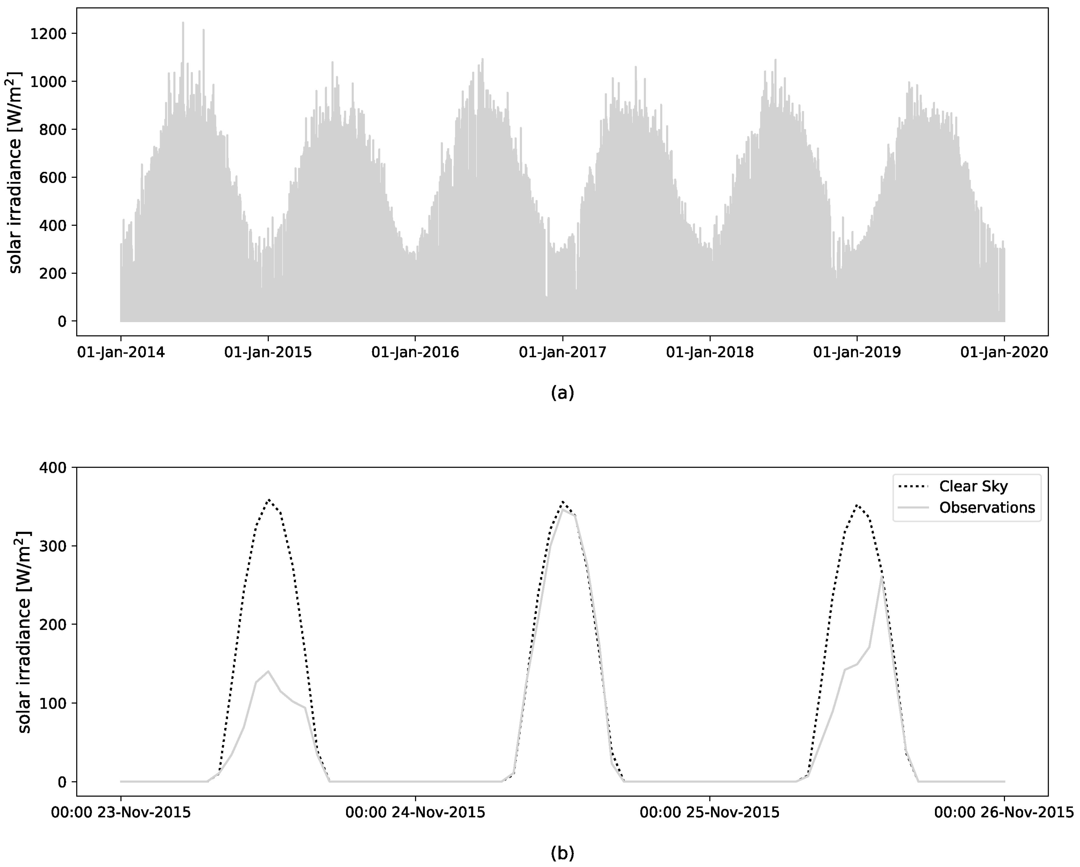
2.3.1. Fluctuation of Solar Radiation

Solar radiation time series, as well as other geophysical signals, belong to the class of the so-called 1/f noises (also known as pink noise), i.e., long-memory processes whose power density spectrum exhibit a slope, α, ranging in [0.5,1.5]. In other words, they are random processes lying between white noise processes, characterized by α = 0, and random walks, characterized by α = 2 (see, for instance [53]). Indeed, the slope of hourly solar irradiance recorded at Como is about α = 1.1 (Figure 2), while the daily average time series exhibits a slope of about α = 0.6, meaning that solar radiation at daily scale is more similar to a white process.
Figure 2 also shows that the power spectral density has some peaks corresponding to periodicity of 24 hours (1.16∙10−5 Hz) and its multiples.

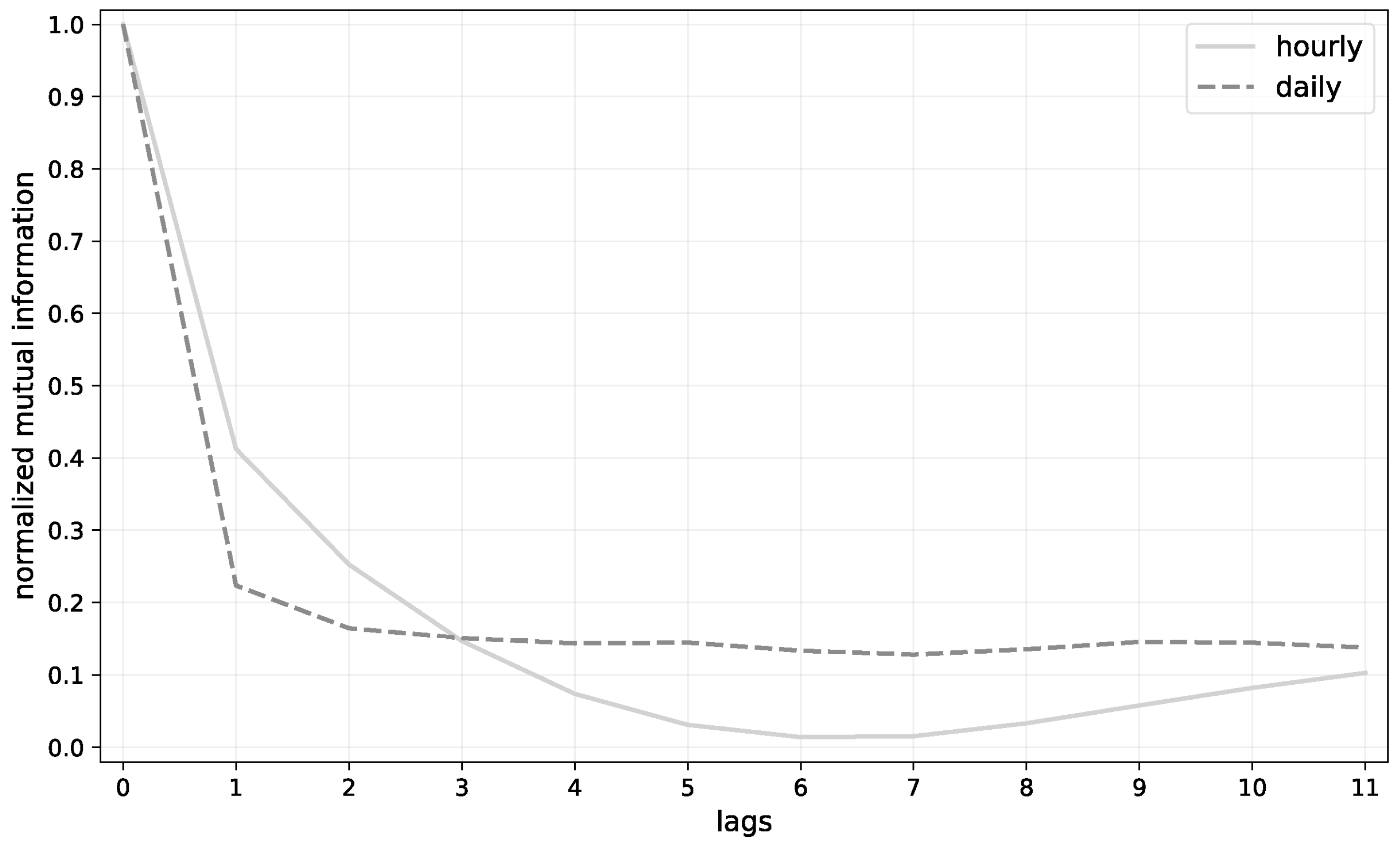
2.3.2. Mutual Information

To capture the nonlinear dependence of solar irradiance time series from its preceding values, we computed the so-called mutual information M(k), defined as in Equation (9) [54].
M ( k ) = i , j p i j ( k ) · l n p i j ( k ) p i p j
In this expression, for some partition of the time series values, pi is the probability to find a time series value in the i-th interval, and pij(k) is the joint probability that an observation falls in the i-th interval, and the observation k time steps later falls into the j-th interval. The partition of the time series can be made with different criteria, for instance by dividing the range of values between the minimum and maximum in a predetermined number of intervals or by taking intervals with equal probability distribution [55]. In our case, we chose to divide the whole range of values into 16 intervals. The normalized mutual information of solar irradiance time series at Como is shown in Figure 3. In the case of Como hourly time series, it gradually decays reaching zero after about six lags. Moreover, it can be observed that the mutual information for the daily values decays more rapidly, thus confirming the greatest difficulty in forecasting solar radiation at a daily scale.

2.4. Benchmark Predictors of Hourly Solar Irradiance

Multi-step ahead forecasting of the global solar irradiance I ( t ) at hourly scale was performed by using models of the form (1–8) defined above.
The performance of such a predictor has been compared with that of some standard baseline models. More specifically, we computed:
  • The “clear sky” model, Clsky in the following, computed as explained in Section 2.2, which represents the average long-term cycle;
  • The so-called Pers24 model expressed as I ^ ( t ) = I ( t 24 ) , which represents the memory linked to the daily cycle;
  • A classical persistent model, Pers in what follows, where I ^ ( t + k ) = I ( t ) ,   k = 1 , 2 , h , representing the component due to a very short-term memory.

2.5. Performance Assessment Metrics

The performances of the various predictors were assessed by computing the following error indices [56]: Bias (10), Mean Absolute Error—MAE (11), Root Mean Square Error—RMSE (12), and R2, also known as Nash-Sutcliffe Efficiency—NSE (13).
B i a s = 1 T t = 1 T ( I ( t ) I ^ ( t ) )
M A E = 1 T t = 1 T | I ( t ) I ^ ( t ) |
R M S E = 1 T t = 1 T ( I ( t ) I ^ ( t ) ) 2
N S E = 1 t = 1 T ( I ( t ) I ^ ( t ) ) 2 t = 1 T ( I ( t ) I ¯ ) 2
where T is the length of the time series, while I ¯ is the average of the observed data.
As concerning to the NSE, an index originally developed for evaluating hydrological models [57], it is worth bearing in mind that it can range from −∞ to 1. An efficiency of 1 (NSE = 1) means that the model perfectly interprets the observed data, while an efficiency of 0 (NSE = 0) indicates that the model predictions are as accurate as the mean of the observed data. It is worth stressing here that, in general, a model is considered sufficiently accurate if NSE > 0.6.
Regardless of what performance index is considered, it is worth noticing that the above classical indicators may overestimate the actual performances of models when applied to the complete time series. When dealing with solar radiation, there is always a strong bias due to the presence of many zero values. In the case at hand, they are about 57% of the sample due to some additional shadowing of the nearby mountains and to the sensitivity of the sensors. When the recorded value is zero, also the forecast is zero (or very close) and all these small errors substantially reduce the average errors and increase the NSE. Additionally, forecasting the solar radiation during the night is useless, and the power network dispatcher may well turn the forecasting model off. In order to overcome this deficiency, which unfortunately is present in many works in the current literature, and allow the models’ performances to be compared when they may indeed be useful, we have also computed the same indicators considering only values above 25 Wm−2 (daytime in what follows), a small value normally reached before dawn and after the sunset. These are indeed the conditions when an accurate energy forecast may turn out to be useful.
Since the Clsky represents what can be forecasted even without using any information about the current situation, it can be assumed as a reference, and the skill index Sf (14) can be computed to measure the improvement gained using the fLSTM and the fFF models:
S f = 1 R M S E f R M S E C l s k y

3. Results

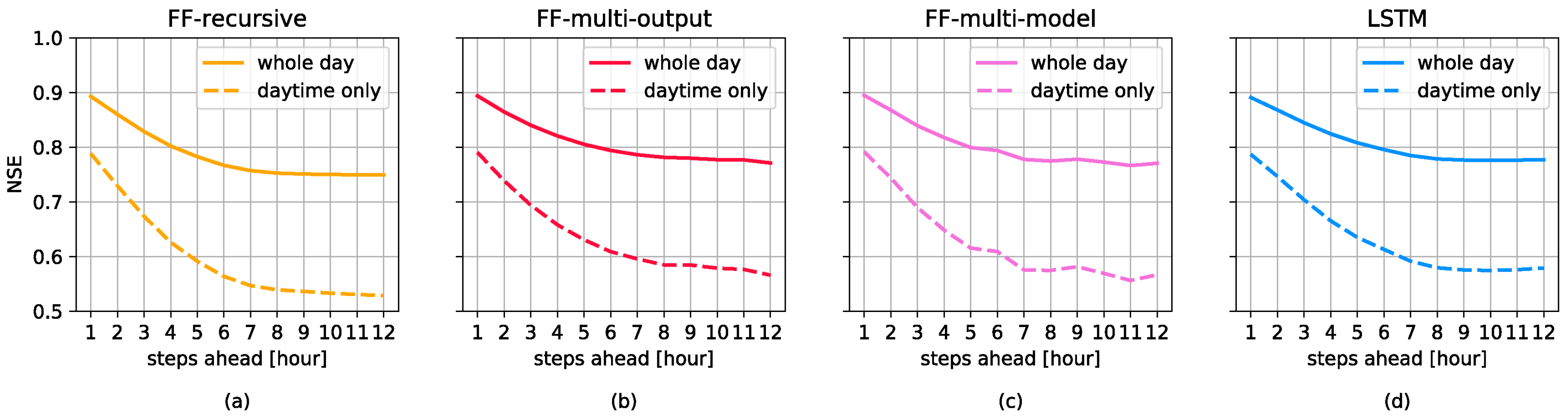
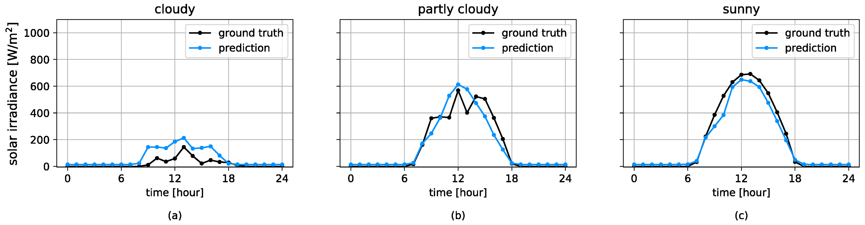
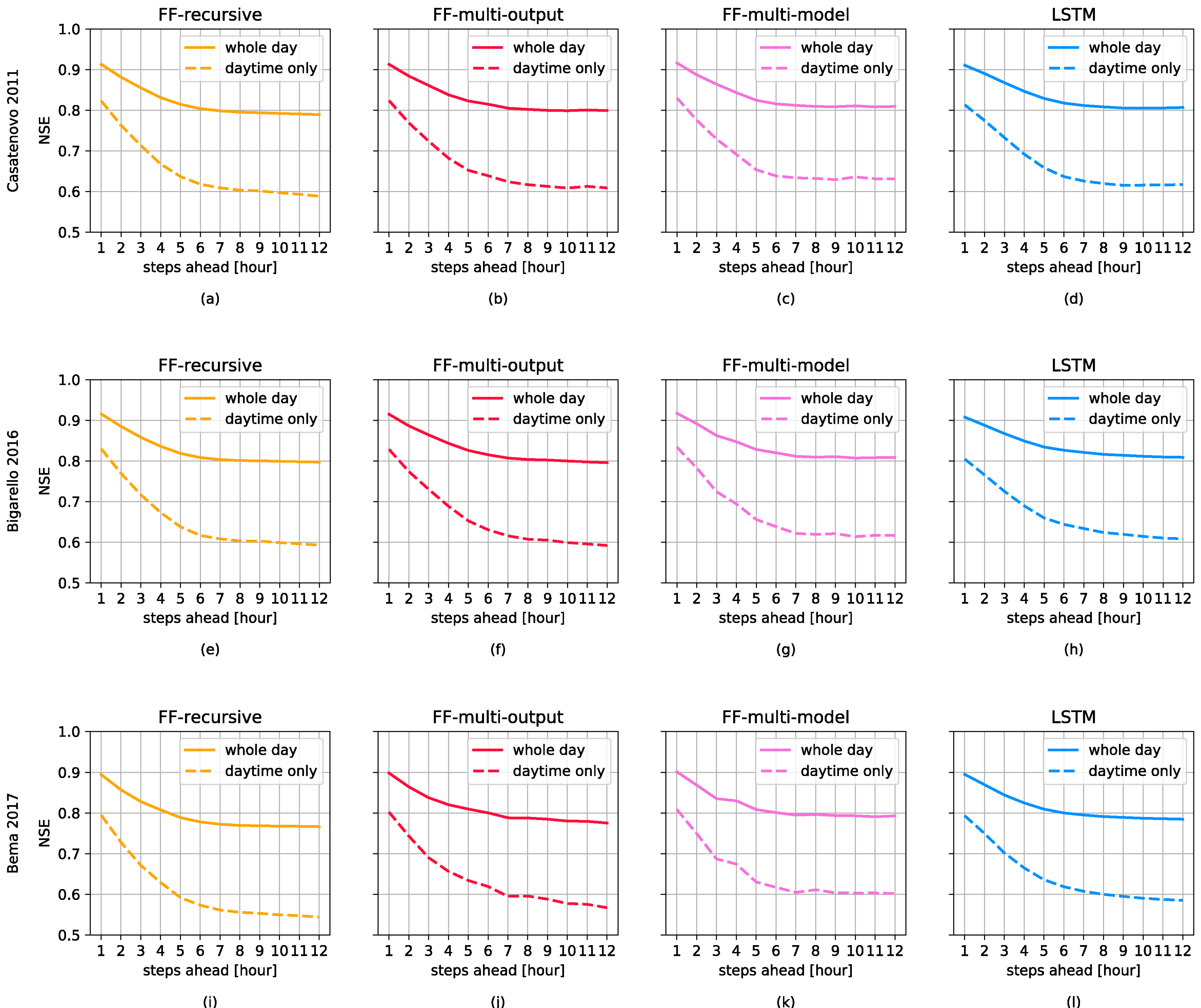
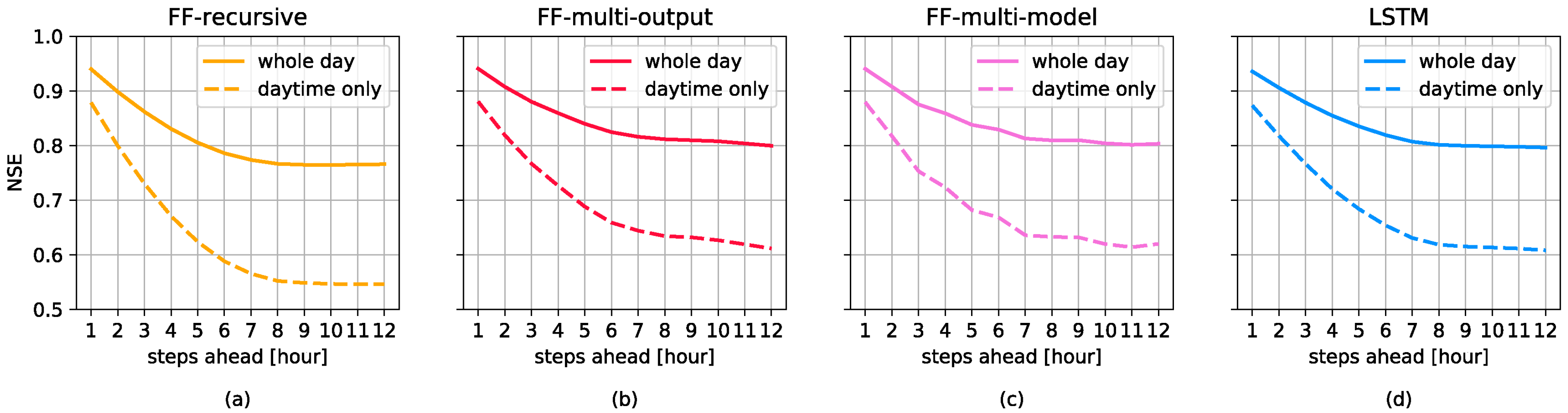
3.1. Forecasting Perfomances

The comparison of the multi-step forecast of solar irradiance with LSTM and FF networks was performed setting the delay parameter d to 24, despite the mutual information indicated that it would be enough to assume d = 6. This choice is motivated by the intrinsic periodicity of solar radiation at an hourly scale [54]. We have experimentally observed that this choice gives more accurate estimates for all the models considered. This probably helps the model in taking into account the natural persistence of solar radiation (see the comments about the performance of the Pers24 model, below). The length of the forecasting horizon h, representing the number of steps ahead we predict in the future, was varied from 1 to 12. Data from 2014 to 2017 were used for network training, 2018 for validating the architecture, and 2019 for testing.
The average performances computed on the first 3 hours of the forecasting horizon of the Pers, Pers24, and Clsky models for the test year 2019 are shown in Table 1 and Table 2. The Pers predictor performance rapidly deteriorate when increasing the horizon. They are acceptable only in the short term: after 1 h, the NSE is equal to 0.79 (considering whole day samples) and 0.59 (daytime samples only), but after two hours NSE decreases to 0.54 (whole day) and 0.14 (daytime only), and six steps ahead the NSE becomes −0.93 (whole day) and −1.64 (daytime). The Pers24 and Clsky preserve the same performances for each step ahead since they are independent on the horizon. Such models inherently take into account the presence of the daily pseudo-periodic component, which affects hourly global solar radiation.
The Pers24 predictor appears to be superior to the Clsky (lower error indicators, higher NSE) confirming that the information of the last 24 h is much more relevant for a correct prediction than the long-term annual cycle. Indeed, the sun position does not change much between one day and the following, and the meteorological conditions have a certain, statistically relevant tendency to persist. Additionally, the Pers24 predictor is the only one with practically zero bias, since the small difference that appears in the first column of Table 1 is simply due to the differences between 31/12/2018 (which is used to compute the predicted values of 1/1/2019) and 31/12/2019. The clear sky model that operates by definition in the absence of cloud cover, overestimates the values above the threshold by 89.86 Wm−2, on average.
From Table 2, it appears that Pers, Pers24 and Clsky, are not reliable models, on average, especially if the NSE is evaluated by using daytime samples only.
Figure 4 reports the results obtained with the three different FF approaches (Figure 4a–c) and the LSTM forecasting model (Figure 4d) in terms of NSE (both in the whole day and in daytime samples only).
Generally speaking, Figure 4 shows that all the considered neural predictors exhibit an NSE which reaches an asymptotic value around six steps ahead. This is coherent with the previous analysis about the mutual information (see Figure 3), which, at an hourly scale, is almost zero after six lags.
If the evaluation is carried out considering whole day samples, all the models would have to be considered reliable enough since NSE is only slightly below 0.8, even for prediction horizons of 12 h. On the contrary, if the evaluation is made considering daytime samples only, it clearly appears that models are reliable for a maximum of 5 h ahead, as for higher horizons the NSE value typically falls below 0.6. Therefore, removing the nighttime values of the time series is decisive for a realistic assessment of a solar radiation forecasting model, that would otherwise be strongly biased.
Going in deeper details, the following considerations can be made.
The FF recursive approach performs slightly worse, particularly as measured by NSE and specifically after a forecasting horizon of 5 h. The FF multi-output and multi-model approaches show performances similar to the LSTM. Additionally, one can note that the performance regularly decreases with the length of the horizon for the FF recursive approach and LSTM net, since they explicitly take into account the sequential nature of the task. Conversely, the FF multi-output and the multi-model ones have irregularities, particularly the latter being each predictor for each specific time horizon completely independent on those on a shorter horizon. If perfect training was possible, such irregularities might perhaps be reduced, but they cannot be completely avoided, particularly on the test dataset, because they are inherent to the approach that considers each predicted value as a separate task.
For all the considered benchmarks and neural predictors, the difference between the whole time series (average value 140.37 Wm−2) and the case with a threshold (daytime only), that excludes nighttime values (average 328.62 Wm−2), emerges clearly, given that during all nights the values are zero or close to it, and thus the corresponding errors are also low.
FF nets and LSTM perform similarly also considering the indices computed along the first 3 h of the forecasting horizon as shown in Table 3 and Table 4, for the whole day and daytime, respectively.
All the neural predictors provide a definite improvement in comparison to the Pers, Pers24, and Clsky models. Looking, for instance, at the NSE the best baseline predictor is the Pers24, scoring 0.63 (whole day) and 0.28 (daytime only). The corresponding values for the neural networks exceed 0.86 and 0.73, respectively.
An in-depth analysis should compare the neural predictors performance at each step with the best benchmark for that specific step. The latter can be considered as an ensemble of benchmarks composed by the the Pers model, the most performing one step ahead (NSE equal to 0.79), and the Pers24 on the following steps (NSE equal to 0.63 for h from 2 to 12). Under this perspective, the neural nets clearly outperform the considered baseline since their NSE score varies from 0.90 to 0.75 (see the solid lines in Figure 4 referring to the whole day). The same analysis performed excluding nighttime values leads to quite similar results, confirming that the neural networks always provide a performance much higher than the benchmarks considered here.
An additional way to examine the model performances is presented in Table 5. We report here the NSE of the predictions of the LSTM network on three horizons, namely 1, 3, and 6 hours ahead. The sunlight (i.e., above 25 W/m2) test series is partitioned into three classes: cloudy, partly cloudy and sunny days, which constitute about 30, 30, and 40% of the sample, respectively. More precisely, cloudy days are defined as those when the daily average irradiance is below 60% of the clear sky index and sunny days those that are above 90% (remember that the clear sky index already accounts for the average sky cloudiness).
It is quite apparent that the performance of the model decreases consistently from sunny, to partly cloudy, to cloudy days. This result is better illustrated in Figure 5 where the 3-hour-ahead predictions are shown for three typical days. In the sunny day, on the right, the process is almost deterministic (governed mainly by astronomical conditions), while the situation is completely different in a cloudy day. In the last case, the forecasting error is of the same order of the process (NSE close to zero) and it can be even larger at 6 hours ahead. This determines the negative NSE value shown in Table 5.

3.2. Domain Adaptation

Besides the accuracy of the forecasted values, another important characteristic of the forecasting models is their generalization capability, often mentioned as domain adaptation in the neural networks literature [58]. This means the possibility of storing knowledge gained while solving one problem and applying it to different, though similar, datasets [59].
To test this feature, the FF and LSTM networks developed for the Como station (source domain) have been used, without retraining, on other sites (target domains) spanning more than one degree of latitude and representing quite different geographical settings: from the low and open plain at 35 m a.s.l. to up the mountains at 800 m a.s.l. In addition, the test year has been changed because solar radiation is far from being truly periodical and some years (e.g., 2017) show significantly higher values than others (e.g., 2011). This means quite different solar radiation encompassing a difference of about 25% between yearly average values.
Figure 6 shows the NSE for the multi-output FF and LSTM networks for three additional stations. All the graphs reach somehow a plateau after six steps ahead, as suggested by the mutual information computed on Como station, and the differences between FF and LSTM networks appear very small or even negligible in almost all the other stations. Six hours ahead, the difference in NSE between Como, for which the networks have been trained, in the test year (2019) and Bema in 2017, which appears to be the most different dataset, is only about 3% for both FF models and LSTM.
As a further trial, both FF models and LSTM have been tested on a slightly different process, i.e., the hourly average solar radiation recorded at the Como station. While the process has the same average of the original dataset, the variability of the process is different since its standard deviation decreased of about 5%. The averaging process indeed filters the high frequencies. Forecasting results are shown in Figure 7. Additionally for this process, the neural models perform more or less as for the hourly values for which they have been trained. The accuracy of both LSTM and FF networks improves by about 0.02 (or 8%) in terms of standard MAE and slightly less in terms of NSE, in comparison to the original process. For a correct comparison with Figure 4, however, it is worth bearing in mind that the 1-hour-ahead prediction corresponds to ( t + 2 ) in the graph, since the average computed at hour ( t + 1 ) is that from ( t ) to ( t + 1 ) and, thus, includes values that are only 5 minutes ahead of the instant at which the prediction is formulated.
An ad-hoc training on each sequence would undoubtedly improve the performance, but the purpose of this section is exactly to show the potential of networks calibrated on different stations, to evaluate the possibility of adopting a predictor developed elsewhere when a sufficiently long series of values is missing. The forecasting models we developed for a specific site could be used with acceptable accuracy for sites were recording stations are not available or existing time series are not long enough. This suggest the possibility of developing a unique forecasting model for the entire region.

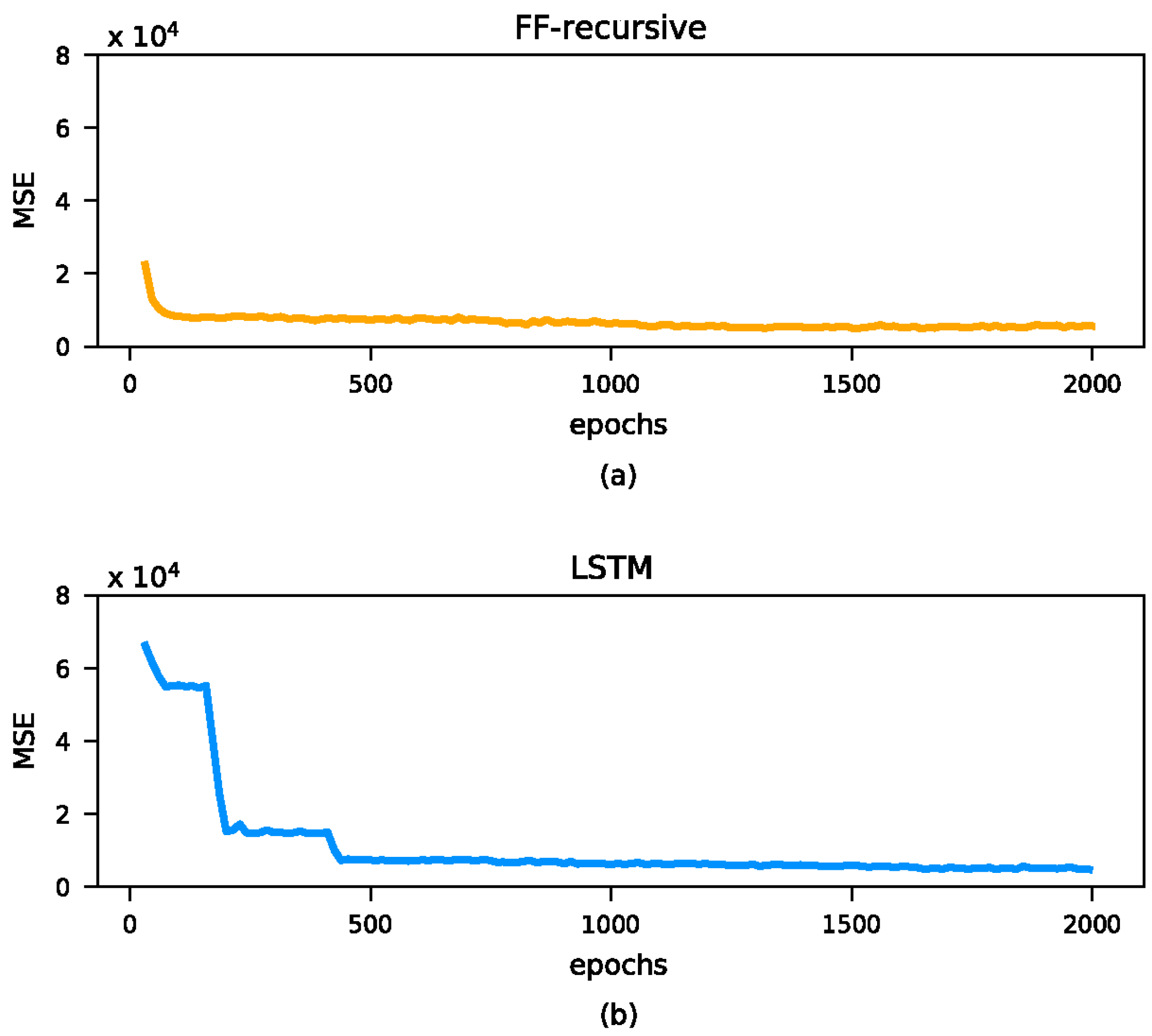
4. Some Remarks on Network Implementations

The development of many successful deep learning models in various applications has been made possible by three joint factors. First, the availability of big data, which are necessary to identify complex models characterized by thousands of parameters. Second, the intuition of making use of fast parallel processing units (GPUs) able to deal with the high computational effort required. Third, the availability of an efficient gradient-based method to train these kinds of neural networks.
This latter are the well-known backpropagation (BP) techniques, which allow efficient computing of the gradients of the loss function with respect to each model weight and bias. To apply the backpropagation of the gradient, it is necessary to have a feed-forward architecture (i.e., without self-loops). In this case, the optimization is extremely efficient since the process can be entirely parallelized, exploiting the GPU.
When the neural architecture presents some loops, as it happens in recurrent cells, the BP technique has to be slightly modified in order fit the new situation. This can be done by unfolding the neural networks through time, to remove self-loops. This extension of BP technique is known as backpropagation through time (BPTT) in the machine learning literature. The issue with BPTT is that the unfolding process should in principle lasts for an infinite number of steps, making the technique useless for practical purposes. For this reason, it is necessary to limit the number of unfolding, considering only the time steps that contain useful information for the prediction (in this case, we say that the BPTT is truncated). As it is easy to understand, BPTT is not as efficient as the traditional BP, because it is not possible to fully parallelize the computation. As a consequence, we are not able to fully exploit the GPU’s computing power, resulting in a slower training. The presence of recurrent units also produces much complex optimization problems due to the presence of a significant number of local optima [60].
Figure 8 shows the substantial difference in the evolution of the training process. As usual, the mean of the quadratic errors of the FF network slowly decreases toward a minimum while this function shows sudden jumps followed by several epochs of stationarity in the case of LSTM. The training algorithm of LSTM can avoid being trapped for too many epochs into local minima, but on the other side, these local minima are more frequent.
For the sake of comparison, we trained the four neural architectures using the same hyperparameters grid, considering the ranges reported in Table 6. As training algorithm, we used the Adam optimizer. Each training procedure has been repeated three times to avoid the problems of an unlucky weights initialization.
While performing similarly under many viewpoints, the FF and LSTM architectures show significant differences if we consider the sensitivity to the hyperparameters values. Figure 9 shows the sensitivity bands obtained for each architecture. The upper bound represents, for each step ahead, the best NSE score achieved across the hyperparameters combinations. The cases in which the optimization process fails due to a strongly inefficient initialization of the weights have been excluded.
The variability of performances of LSTM across the hyperparameter space is quite limited if compared with that of FF architectures. This is probably because the LSTM presents a sequential structure and is optimized on the whole 12-step-forecasting horizon. The recursive FF model is identified as the optimal one-step ahead predictor, and thus there are some cases characterized by poor performances in the rest of the horizon. The multi-output and multi-model FF seem to suffer of the same problem because, as already pointed out, they predict the values at each time step as independent variables.

5. Conclusions

The availability of accurate multi-step ahead forecast of solar irradiance (and, hence, power) is of extreme importance for the efficient balancing and management of power networks since they allow the implementation of accurate and efficient control procedures, such as model predictive control.
The results reported in this study further confirm the well-known accuracy of FF and LSTM networks for the above purpose and, more in general, in predicting time series related to environmental variables. Another interesting conclusion is that among the Rec, MM and MO models, the Rec is the one that exhibits the lowest performances. A rough explanation probably lies in the fact that its parameters are optimized over a time horizon of 1 step, but then artificially used for a longer horizon, thus propagating the error. Therefore one of the merits of this study is to clarify that a common practice, namely to identify a model of the type x ( t + 1 ) = f ( x ( t ) ) , to then predict x ( t + h ) is not the best choice. To this end, the proposed MM and MO may represent alternatives that are more appropriate.
However, such good performances are obtained at a cost in terms of data and time required to train the network. In actual applications, one has to trade these costs versus the improvement in the precision of the forecasting. In this respect, the solution which appears to be a trade-off between accuracy and complexity seems to be the MO. Indeed, it can reach a very good performance with a minimum increment of the number of parameters compared to the recursive approach. The MM approach performs slightly better than the MO one but requires a different training (and possibly, a different architecture) for each forecasting horizon, which, in the present study, means training over a million parameters.
In more general terms, the selection of the forecasting model should be made by looking at the comparative advantages that a better precision provides versus the effort to obtain such a precision. Though the economic cost and the computation time required to synthesize even a very complex LSTM network are already rather low and still decreasing, one may also consider adopting a classical FF neural network model, which outperforms the traditional Pers24 model and is much easier to train with respect to the corresponding LSTM.
Another of the peculiarities of this work has been showing how performance indices are strongly affected by the presence of null values and, in this respect, nighttime samples should be removed for a correct assessment of model performances.
Both FF and LSTM networks developed in this study have proved to be able to forecast solar radiation in other stations of a relatively wide domain with a minimal loss of precision and without the need to retrain them. This opens the way to the development of county or regional predictors, valid for ungauged locations with different geographical settings. Such precision may perhaps be further improved by using other meteorological data as input to the model, thus extending the purely autoregressive approach adopted in this study.

Author Contributions

Conceptualization, G.G., G.N. and M.S.; methodology, G.G., G.N. and M.S.; software, M.S.; validation, G.G., G.N. and M.S.; data curation, G.G., G.N. and M.S.; writing—original draft preparation, G.G., G.N. and M.S.; writing—review and editing, G.G., G.N. and M.S.; visualization, M.S.; supervision, G.G. and G.N. All authors have read and agreed to the published version of the manuscript.

Funding

This research received no external funding.

Conflicts of Interest

The authors declare no conflict of interest.

References

  1. Shah, A.S.B.M.; Yokoyama, H.; Kakimoto, N. High-precision forecasting model of solar irradiance based on grid point value data analysis for an efficient photovoltaic system. IEEE Trans. Sustain. Energy 2015, 6, 474–481. [Google Scholar] [CrossRef]
  2. Urrego-Ortiz, J.; Martínez, J.A.; Arias, P.A.; Jaramillo-Duque, Á. Assessment and Day-Ahead Forecasting of Hourly Solar Radiation in Medellín, Colombia. Energies 2019, 12, 4402. [Google Scholar] [CrossRef] [Green Version]
  3. Mpfumali, P.; Sigauke, C.; Bere, A.; Mulaudzi, S. Day Ahead Hourly Global Horizontal Irradiance Forecasting—Application to South African Data. Energies 2019, 12, 3569. [Google Scholar] [CrossRef] [Green Version]
  4. Mohamed, A.; Salehi, V.; Ma, T.; Mohammed, O. Real-time energy management algorithm for plug-in hybrid electric vehicle charging parks involving sustainable energy. IEEE Trans. Sustain. Energy 2014, 5, 577–586. [Google Scholar] [CrossRef]
  5. Bhatti, A.R.; Salam, Z.; Aziz, M.J.B.A.; Yee, K.P.; Ashique, R.H. Electric vehicles charging using photovoltaic: Status and technological review. Renew. Sustain. Energy Rev. 2016, 54, 34–47. [Google Scholar] [CrossRef]
  6. Sáez, D.; Ávila, F.; Olivares, D.; Cañizares, C.; Marín, L. Fuzzy prediction interval models for forecasting renewable resources and loads in microgrids. IEEE Trans. Smart Grid 2015, 6, 548–556. [Google Scholar]
  7. Yadav, A.K.; Chandel, S.S. Solar radiation prediction using Artificial Neural Network techniques: A review. Renew. Sustain. Energy Rev. 2014, 772–781. [Google Scholar] [CrossRef]
  8. Wan, C.; Zhao, J.; Song, Y.; Xu, Z.; Lin, J.; Hu, Z. Photovoltaic and solar power forecasting for smart grid energy management. CSEE J. Power Energy Syst. 2015, 1, 38–46. [Google Scholar] [CrossRef]
  9. Voyant, C.; Notton, G.; Kalogirou, S.; Nivet, M.; Paoli, C.; Motte, F.; Fouilloy, A. Machine learning methods for solar radiation forecasting: A review. Renew. Energy 2017, 105, 569–582. [Google Scholar] [CrossRef]
  10. Sobri, S.; Koohi-Kamali, S.; Rahim, N.A. Solar photovoltaic generation forecasting methods: A review. Energy Convers. Manag. 2018, 156, 459–497. [Google Scholar] [CrossRef]
  11. Sun, H.; Yan, D.; Zhao, N.; Zhou, J. Empirical investigation on modeling solar radiation series with ARMA–GARCH models. Energy Convers. Manag. 2015, 92, 385–395. [Google Scholar] [CrossRef]
  12. Lauret, P.; Boland, J.; Ridley, B. Bayesian statistical analysis applied to solar radiation modelling. Renew. Energy 2013, 49, 124–127. [Google Scholar] [CrossRef]
  13. Kwon, Y.; Kwasinski, A.; Kwasinski, A. Solar Irradiance Forecast Using Naïve Bayes Classifier Based on Publicly Available Weather Forecasting Variables. Energies 2019, 12, 1529. [Google Scholar] [CrossRef] [Green Version]
  14. Piri, J.; Kisi, O. Modelling solar radiation reached to the earth using ANFIS, NN-ARX, and empirical models (case studies: Zahedan and Bojnurd stations). J. Atmos. Solar Terr. Phys. 2015, 123, 39–47. [Google Scholar] [CrossRef]
  15. Gholipour, A.; Lucas, C.; Araabi, B.N.; Mirmomeni, M.; Shafiee, M. Extracting the main patterns of natural time series for long-term neurofuzzy prediction. Neural Comput. Appl. 2007, 16, 383–393. [Google Scholar] [CrossRef]
  16. Dawan, P.; Sriprapha, K.; Kittisontirak, S.; Boonraksa, T.; Junhuathon, N.; Titiroongruang, W.; Niemcharoen, S. Comparison of Power Output Forecasting on the Photovoltaic System Using Adaptive Neuro-Fuzzy Inference Systems and Particle Swarm Optimization-Artificial Neural Network Model. Energies 2020, 13, 351. [Google Scholar] [CrossRef] [Green Version]
  17. Kisi, O. Modeling solar radiation of Mediterranean region in Turkey by using fuzzy genetic approach. Energy 2014, 64, 429–436. [Google Scholar] [CrossRef]
  18. Shakya, A.; Michael, S.; Saunders, C.; Armstrong, D.; Pandey, P.; Chalise, S.; Tonkoski, R. Solar irradiance forecasting in remote microgrids using Markov switching model. IEEE Trans. Sustain. Energy 2017, 8, 895–905. [Google Scholar] [CrossRef]
  19. Sharma, N.; Sharma, P.; Irwin, D.; Shenoy, P. Predicting solar generation from weather forecasts using machine learning. In Proceedings of the IEEE International Conference on Smart Grid Communications (SmartGridComm), Brussels, Belgium, 17–20 October 2011; pp. 528–533. [Google Scholar]
  20. Hassan, M.Z.; Ali, M.E.K.; Ali, A.S.; Kumar, J. Forecasting Day-Ahead Solar Radiation Using Machine Learning Approach. In Proceedings of the 4th Asia-Pacific World Congress on Computer Science and Engineering (APWC on CSE), Mana Island, Fiji, 11–13 December 2017; pp. 252–258. [Google Scholar]
  21. Bae, K.Y.; Jang, H.S.; Sung, D.K. Hourly solar irradiance prediction based on support vector machine and its error analysis. IEEE Trans. Power Syst. 2017, 32, 935–945. [Google Scholar] [CrossRef]
  22. Capizzi, G.; Napoli, C.; Bonanno, F. Innovative second-generation wavelets construction with recurrent neural networks for solar radiation forecasting. IEEE Trans. Neural Netw. Learn. Syst. 2012, 23, 1805–1815. [Google Scholar] [CrossRef] [Green Version]
  23. Lotfi, M.; Javadi, M.; Osório, G.J.; Monteiro, C.; Catalão, J.P.S. A Novel Ensemble Algorithm for Solar Power Forecasting Based on Kernel Density Estimation. Energies 2020, 13, 216. [Google Scholar] [CrossRef] [Green Version]
  24. McCandless, T.; Dettling, S.; Haupt, S.E. Comparison of Implicit vs. Explicit Regime Identification in Machine Learning Methods for Solar Irradiance Prediction. Energies 2020, 13, 689. [Google Scholar] [CrossRef] [Green Version]
  25. Crisosto, C.; Hofmann, M.; Mubarak, R.; Seckmeyer, G. One-Hour Prediction of the Global Solar Irradiance from All-Sky Images Using Artificial Neural Networks. Energies 2018, 11, 2906. [Google Scholar] [CrossRef] [Green Version]
  26. Ji, W.; Chee, K.C. Prediction of hourly solar radiation using a novel hybrid model of ARMA and TDNN. Solar Energy 2011, 85, 808–817. [Google Scholar] [CrossRef]
  27. Zhang, N.; Behera, P.K. Solar radiation prediction based on recurrent neural networks trained by Levenberg-Marquardt backpropagation learning algorithm. In Proceedings of the 2012 IEEE PES Innovative Smart Grid Technologies (ISGT), Washington, DC, USA, 16–20 January 2012; pp. 1–7. [Google Scholar]
  28. Zhang, N.; Behera, P.K.; Williams, C. Solar radiation prediction based on particle swarm optimization and evolutionary algorithm using recurrent neural networks. In Proceedings of the IEEE International Systems Conference (SysCon), Orlando, FL, USA, 15–18 April 2013; pp. 280–286. [Google Scholar]
  29. Jaihuni, M.; Basak, J.K.; Khan, F.; Okyere, F.G.; Arulmozhi, E.; Bhujel, A.; Park, J.; Hyun, L.D.; Kim, H.T. A Partially Amended Hybrid Bi-GRU—ARIMA Model (PAHM) for Predicting Solar Irradiance in Short and Very-Short Terms. Energies 2020, 13, 435. [Google Scholar] [CrossRef] [Green Version]
  30. Zang, H.; Cheng, L.; Ding, T.; Cheung, K.W.; Liang, Z.; Wei, Z.; Sun, G. Hybrid method for short-term photovoltaic power forecasting based on deep convolutional neural network. IET Generation Transm. Distrib. 2018, 12, 4557–4567. [Google Scholar] [CrossRef]
  31. Yona, A.; Senjyu, T.; Funabashi, T.; Kim, C. Determination method of insolation prediction with fuzzy and applying neural network for long-term ahead PV power output correction. IEEE Trans. Sustain. Energy 2013, 4, 527–533. [Google Scholar] [CrossRef]
  32. Yang, H.; Huang, C.; Huang, Y.; Pai, Y. A weather-based hybrid method for 1-day ahead hourly forecasting of PV power output. IEEE Trans. Sustain. Energy 2014, 5, 917–926. [Google Scholar] [CrossRef]
  33. Liu, J.; Fang, W.; Zhang, X.; Yang, C. An improved photovoltaic power forecasting model with the assistance of aerosol index data. IEEE Trans. Sustain. Energy 2015, 6, 434–442. [Google Scholar] [CrossRef]
  34. Ehsan, R.M.; Simon, S.P.; Venkateswaran, P.R. Day-ahead forecasting of solar photovoltaic output power using multilayer perceptron. Neural Comput. Appl. 2017, 28.12, 3981–3992. [Google Scholar] [CrossRef]
  35. Wojtkiewicz, J.; Hosseini, M.; Gottumukkala, R.; Chambers, T.L. Hour-Ahead Solar Irradiance Forecasting Using Multivariate Gated Recurrent Units. Energies 2019, 12, 4055. [Google Scholar] [CrossRef] [Green Version]
  36. Abdel-Nasser, M.; Mahmoud, K. Accurate photovoltaic power forecasting models using deep LSTM-RNN. Neural Comput. Appl. 2019, 31, 2727–2740. [Google Scholar] [CrossRef]
  37. Lai, G.; Chang, W.; Yang, Y.; Liu, H. Modeling long-and short-term temporal patterns with deep neural networks. In Proceedings of the 41st International Conference on Research and Development in Information Retrieval, Ann Arbor, MI, USA, 8–12 July 2018; pp. 95–104. [Google Scholar]
  38. Maitanova, N.; Telle, J.-S.; Hanke, B.; Grottke, M.; Schmidt, T.; Maydell, K.; Agert, C. A Machine Learning Approach to Low-Cost Photovoltaic Power Prediction Based on Publicly Available Weather Reports. Energies 2020, 13, 735. [Google Scholar] [CrossRef] [Green Version]
  39. Fouilloy, A.; Voyant, C.; Notton, G.; Motte, F.; Paoli, C.; Nivet, M.L.; Guillot, E.; Duchaud, J.L. Solar irradiation prediction with machine learning: Forecasting models selection method depending on weather variability. Energy 2020, 165, 620–629. [Google Scholar] [CrossRef]
  40. Notton, G.; Voyant, C.; Fouilloy, A.; Duchaud, J.L.; Nivet, M.L. Some applications of ANN to solar radiation estimation and forecasting for energy applications. Appl. Sci. 2019, 9, 209. [Google Scholar] [CrossRef] [Green Version]
  41. Husein, M.; Chung, I.-Y. Day-Ahead Solar Irradiance Forecasting for Microgrids Using a Long Short-Term Memory Recurrent Neural Network: A Deep Learning Approach. Energies 2019, 12, 1856. [Google Scholar] [CrossRef] [Green Version]
  42. Aslam, M.; Lee, J.-M.; Kim, H.-S.; Lee, S.-J.; Hong, S. Deep Learning Models for Long-Term Solar Radiation Forecasting Considering Microgrid Installation: A Comparative Study. Energies 2020, 13, 147. [Google Scholar] [CrossRef] [Green Version]
  43. Dercole, F.; Sangiorgio, M.; Schmirander, Y. An empirical assessment of the universality of ANNs to predict oscillatory time series. IFAC-PapersOnLine 2020, in press. [Google Scholar]
  44. Sangiorgio, M.; Dercole, F. Robustness of LSTM Neural Networks for Multi-step Forecasting of Chaotic Time Series. Chaos Solitons Fractals 2020, 139, 110045. [Google Scholar] [CrossRef]
  45. Hochreiter, S.; Schmidhuber, J. Long short-term memory. Neural Comput. 1997, 9, 1735–1780. [Google Scholar] [CrossRef]
  46. Schmidhuber, J. Deep learning in neural networks: An overview. Neural Netw. 2015, 61, 85–117. [Google Scholar] [CrossRef] [PubMed] [Green Version]
  47. Goodfellow, I.; Bengio, Y.; Courville, A. Deep Learning; MIT Press: Cambridge, MA, USA, 2016. [Google Scholar]
  48. Chollet, F. Keras: The python deep learning library. Astrophysics Source Code Library. Available online: https://keras.io (accessed on 25 June 2020).
  49. Paszke, A.; Gross, S.; Massa, F.; Lerer, A.; Bradbury, J.; Chanan, G.; Killeen, T.; Lin, Z.; Gimelshein, N.; Antiga, L.; et al. PyTorch: An imperative style, high-performance deep learning library. Adv. Neural Inf. Process. Syst. 2019, 8024–8035. [Google Scholar]
  50. Ineichen, P.; Perez, R. A new airmass independent formulation for the Linke turbidity coefficient. Solar Energy 2012, 73, 151–157. [Google Scholar] [CrossRef] [Green Version]
  51. Perez, R.; Ineichen, P.; Moore, K.; Kmiecik, M.; Chain, C.; George, R.; Vignola, F. A new operational model for satellite-derived irradiances: Description and validation. Solar Energy 2002, 73, 307–317. [Google Scholar] [CrossRef] [Green Version]
  52. PV Performance Modeling Collaborative. Available online: https://pvpmc.sandia.gov (accessed on 2 May 2020).
  53. Miramontes, O.; Rohani, P. Estimating 1/fα scaling exponents from short time-series. Phys. D Nonlinear Phenom. 2002, 166, 147–154. [Google Scholar] [CrossRef]
  54. Fortuna, L.; Nunnari, G.; Nunnari, S. Nonlinear Modeling of Solar Radiation and Wind Speed Time Series; Springer International Publishing: Cham, Switzerland, 2016. [Google Scholar]
  55. Jiang, A.H.; Huang, X.C.; Zhang, Z.H.; Li, J.; Zhang, Z.Y.; Hua, H.X. Mutual information algorithms. Mech. Syst. Signal Process. 2010, 24, 2947–2960. [Google Scholar] [CrossRef]
  56. Zhang, J.; Florita, A.; Hodge, B.M.; Lu, S.; Hamann, H.F.; Banunarayanan, V.; Brockway, A.M. A suite of metrics for assessing the performance of solar power forecasting. Solar Energy 2015, 111, 157–175. [Google Scholar] [CrossRef] [Green Version]
  57. Nash, J.E.; Sutcliffe, J.V. River flow forecasting through conceptual models part I—A discussion of principles. J. Hydrol. 1970, 10, 282–290. [Google Scholar] [CrossRef]
  58. Glorot, X.; Bordes, A.; Bengio, Y. Domain adaptation for large-scale sentiment classification: A deep learning approach. In Proceedings of the 28th international conference on machine learning (ICML), Bellevue, DC, USA, 28 June–2 July 2011; pp. 513–520. [Google Scholar]
  59. Yosinski, J.; Clune, J.; Bengio, Y.; Lipson, H. How transferable are features in deep neural networks? Adv. Neural Inf. Process. Syst. 2014, 3320–3328. [Google Scholar]
  60. Cuéllar, M.P.; Delgado, M.; Pegalajar, M.C. An application of non-linear programming to train recurrent neural networks in time series prediction problems. In Proceedings of the 7th International Conference on Enterprise Information Systems (ICEIS), Miami, FL, USA, 24–28 May 2005; pp. 95–102. [Google Scholar]
Figure 1. Hourly solar irradiance time series (a), compared with clear sky values for a few specific days (b).
Energies 13 03987 g001
Figure 2. Power spectral density of the hourly solar irradiance (grey) and trend 1/fα characterized by α = 1.1 (black).
Energies 13 03987 g002
Figure 3. Normalized mutual information of hourly and daily solar irradiance at Como.
Energies 13 03987 g003
Figure 4. NSE of hourly solar irradiance at Como obtained with recursive FF (a), multi-output FF (b), multi-model FF (c), and LSTM (d). Solid line represents the performance in the whole day, dashed line in daytime only. Values refer to the test year 2019.
Energies 13 03987 g004
Figure 5. Three-hour-ahead LSTM predictions versus observations in three typical days with different cloudiness: a cloudy day (a), a partly cloudy day (b), and a sunny day (c). Values refer to the test year (2019).
Energies 13 03987 g005
Figure 6. NSE of hourly solar irradiance forecast at Casatenovo (ad) in 2011, Bigarello (eh) in 2016, and Bema (il) in 2017. Each column is relative to a different neural predictor. Solid line represents the performance in the whole day, dashed line in daytime only.
Energies 13 03987 g006
Figure 7. NSE of hourly average solar irradiance at Como obtained with recursive FF (a), multi-output FF (b), multi-model FF (c), and LSTM (d). Solid line represents the performance in the whole day, dashed line in daytime only. Values refer to the test year (2019).
Energies 13 03987 g007
Figure 8. Evolution of the MSE across the training epochs for recursive FF (a) and LSTM (b) predictors.
Energies 13 03987 g008
Figure 9. Sensitivity bands obtained with FF-recursive (a), FF-multi-output (b), FF-multi-model (c), and LSTM (d) on the 12-step-ahead prediction. Values refer to the test year (2019).
Energies 13 03987 g009
Table 1. Average performances of the Pers, Pers24, and Clsky predictors on the first 3 hours (whole day).
IndexPersPers24Clsky
Bias0.070.01−46.20
MAE87.7859.2474.07
RMSE158.40136.63146.39
NSE0.510.630.58
Table 2. Average performances of the Pers, Pers24, and Clsky predictors on the first 3 hours (daytime samples only).
IndexPersPers24Clsky
Bias28.827.08−89.91
MAE175.89131.71154.35
RMSE228.24204.91212.97
NSE0.110.280.22
Table 3. Average performances of FF and LSTM predictors on the first 3 hours (whole day).
IndexFF-RecursiveFF-Multi-OutputFF-Multi-ModelLSTM
Bias−1.49−0.280.17−4.19
MAE40.2640.3939.2645.91
RMSE84.3382.6082.2982.09
NSE0.860.870.870.87
S0.420.440.440.44
Table 4. Average performances of FF and LSTM predictors on the first 3 hours (daytime samples only).
IndexFF-RecursiveFF-Multi-OutputFF-Multi-ModelLSTM
Bias3.796.596.4612.11
MAE86.3184.6384.7586.01
RMSE125.35122.87122.74121.78
NSE0.730.740.740.75
S0.410.420.420.43
Table 5. LSTM performances in terms of NSE for cloudy, partly cloudy and sunny days (daytime samples only).
Index1 Hour Ahead3 Hours Ahead6 Hours Ahead
Cloudy0.440.06−0.45
Partly cloudy0.650.590.59
Sunny0.890.830.73
Table 6. Hyperparameters values considered in the grid-search tuning process for FF and LSTM predictors.
HyperparameterSearch RangeOptimal Values
FF-RecursiveFF-Multi-OutputFF-Multi-ModelLSTM
Hidden layers3–53553
Neurons per layer5–10510105
Learning rate10−2–10−310−310−210−210−3
Decay rate0–10−4010−410−410−4
Batch size128–512512128512512

