Synergies between e-Mobility and Photovoltaic Potentials—A Case Study on an Urban Medium Voltage Grid

Abstract

To reduce CO₂ emissions, it is necessary to cover the increasing energy demand of e-mobility with renewable energy sources. Therefore, the influence of increasing e-mobility and synergy effects between e-mobility and renewable energy sources need to be investigated. The case study presented here shows results from the analysis of grid-side and energetic synergy effects between e-mobility charged only at work and photovoltaic (PV) potentials. The basis of the grid study is a simplified cell-based grid model. Following the determination of synthetic charging profiles for e-mobility, PV potential profiles, load and production profiles, we perform load flow calculations for different scenarios and a simulation period of one year using the grid model. After the grid study, the energy analyses are carried out using four key performance indicators. The grid study shows that line overloads caused by PV production are only reduced and not avoided by increasing e-mobility and vice versa. The increase in the power peak of e-mobility, by shifting the charging processes into the peak of PV potentials, leads to a reduction of the production surplus in summer, while in winter the line utilisation increases. By modelling PV potentials on real irradiation and temperature data, the investigation of key performance indicators can identify not only seasonal fluctuations but also daily fluctuations.

1. Introduction

To contribute to the reduction of CO₂ emissions, it is necessary to change over to alternative drive systems such as electric vehicles (EV) in the transport sector. The change to e-mobility leads to an increasing electricity demand, which can lead to a reduction of grid stability and security of supply [1,2,3,4,5]. The additional electricity demand of electric vehicles must be provided by renewable energy sources (RES) to achieve decarbonisation targets. The impact of the EVs electricity demand together with the fluctuating RES production can lead to additional challenges compared to a single consideration of e-mobility [6,7,8,9]. Munkhammar et al. [6] focused on home charging and investigated the interaction between the household power consumption, the electric vehicle home charging and the photovoltaic (PV) power production using a probability model. The investigation shows on the one hand the increasing peak load caused by EV charging and on the other hand, the time-shift between EV charging and PV power production. This time-shift is based on the fact that the PV power production and the resulting peak is available during the day, while the peak caused by charging at home occurs in the evening. To reduce this shift and thereby increase power self-consumption, a change in the user behaviour of EV drivers or the application of demand side measures becomes necessary. For a better use of the PV power production, stays during the day should be used for charging the EVs, such as charging at work and charging commercially. [10] Since the load profiles of e-mobility and thus the required charging infrastructure are strongly dependent on respective user behaviour of EV drivers [1,11], load shift potentials of electric vehicles for different available charging infrastructures (e.g., for charging at home vs. for charging at work) are determined in the references [10,12]. Even with an uncontrolled charging, the PV power production can be better utilised when charging at work compared to charging at home. This is caused by the fact that charging at work is usually performed during the day, while charging at home is generally performed in the evening-hours and at night. [10] Babrowski et al. [12] conclude that the greatest potential for controlled charging is in the area of workplace charging using PV power production.

Despite the large number of presented approaches and results on the interaction between PV power production and uncontrolled and controlled EV charging, to the best of our knowledge, the impact of this interaction on the distribution grids have not yet been sufficiently studied. Therefore, the case study presented in this paper will focus on charging at work and the impact of different penetrations of work-charged EVs and PV potentials on an urban medium-voltage grid. For this purpose, we have developed a grid model for the medium-voltage grid of a medium-sized city based on a cellular approach, using the example of Leoben in Austria. The application of the cellular approach simplifies the complex grid structure and allows reduced calculation times. The approach is therefore suitable for usually time-consuming time resolved load flow calculations, e.g., with annual load profiles. [11] Besides the modelling of existing consumer and producer profiles, we determine production profiles of PV potentials and synthetic charging load profiles of e-mobility. While Su et. al. [13], for example, characterise PV production profiles by averages of “rainy days”, “cloudy days” and “sunny days”, the case study presented here determines the time-resolved production profiles of PV potentials (15-minute mean value) for each calendar day on the basis of irradiation and temperature data [14] and a solar roof register depicting the actual roof areas [15]. The determination of synthetic charging load profiles for e-mobility is based on traffic analysis, mobility pattern and statistical data. [11] The method for this determination, we have already shown in [11], has been extended in this work, among others, by the function of taking controlled charging into account. In comparison to Gnann et al. [10], where summer charging is shifted to midday and in winter the focus is on peak-shaving by charging at night, here a combination of the summer and winter strategy for controlled charging is applied, regardless of the season. The method distinguishes between shifting the charging process into the peak of the PV production profile or, distributing the charging processes over a defined period of time. For each charging process, it is decided separately if it can be shifted under the defined parameters (for example duration of stay and distance travelled) into the intended period of controlled charging. By comparing the scenarios for uncontrolled charging with those of controlled charging, we investigate in addition to the energetic benefits for the direct use of PV production, whether controlled charging can prevent the negative effects of uncontrolled charging on the power grid. The focus of this analysis is therefore to determine the benefits of controlled charging on the existing infrastructure considering today’s mobility behaviour, while Zhang and Chen [16] discuss smart charging management based on mobility behaviour and regional energy prices. Using the cell-based grid model and the determined annual load and production profiles, we perform time resolved load flow calculations for different scenarios. The scenarios differ between the penetrations of e-mobility and PV potentials, the charging power as well as controlled and uncontrolled charging. Based on the results of the load flow calculations, we present grid-side synergy effects and energy-related key performance indicators between e-mobility and PV potentials for the different scenarios.

2. Data Description

In this section, all data required for the case study and its preparation is presented. Starting with the description of the medium-voltage grid of the city of Leoben, the data required to model the synthetic charging load profiles for e-mobility are presented. This includes traffic analyses, mobility patterns and vehicle-related specifications. Finally, the fundamental data for modelling the PV potential profiles are described.

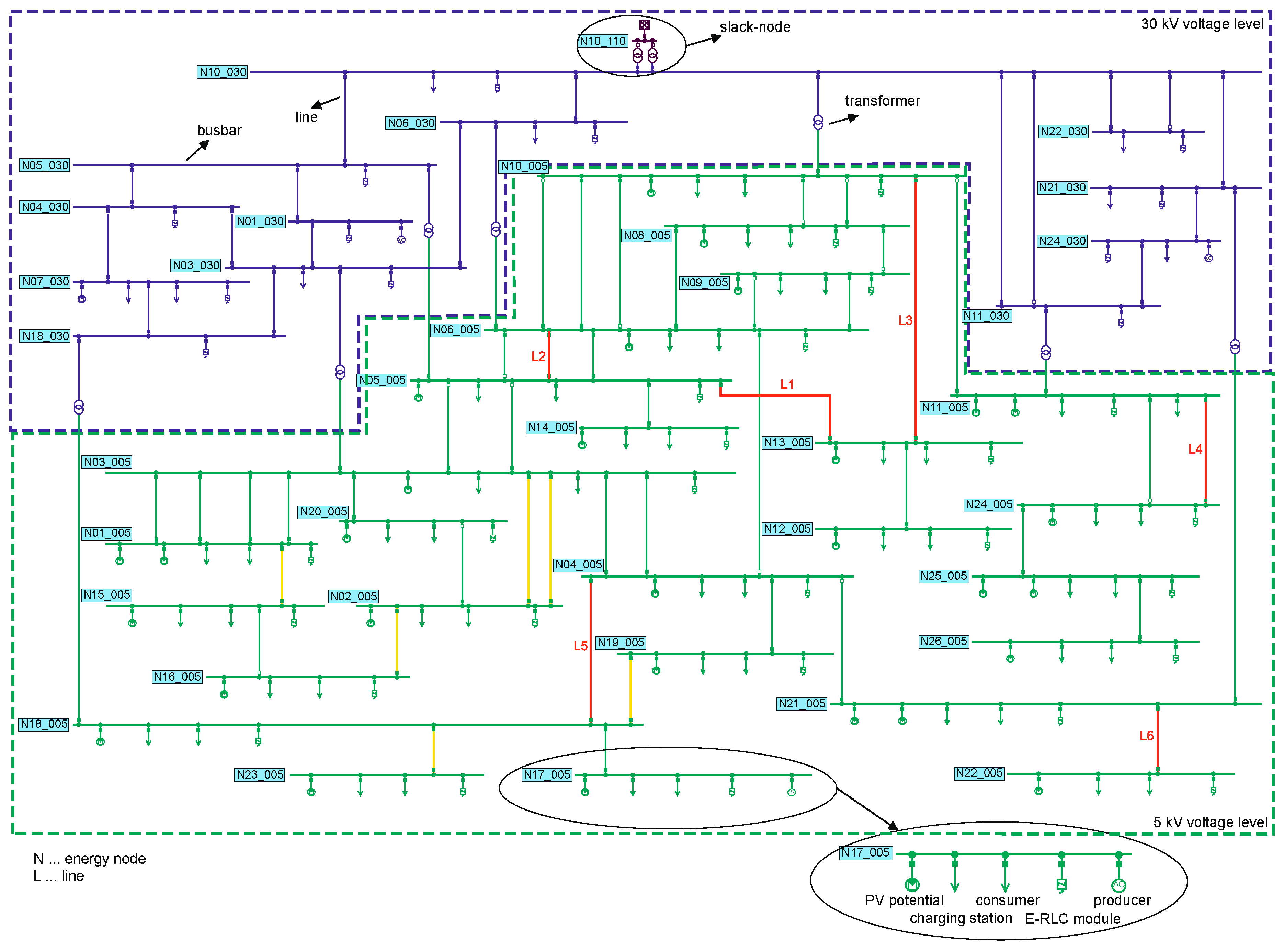
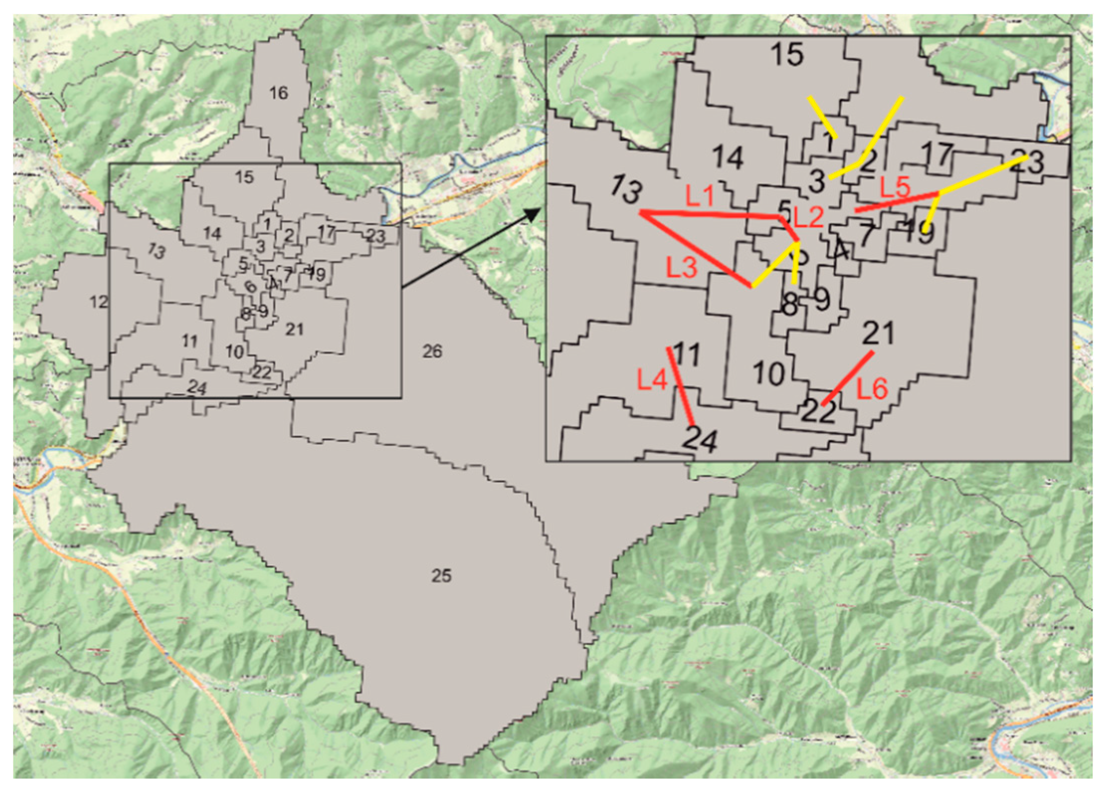
2.1. Medium-Voltage Grid

The original medium-voltage grid for the city of Leoben within the framework of the Austrian research funding agency (FFG) projects “Smart Exergy Leoben” [17] and “Move2Grid” [18] has been anonymised and made available by the local grid operator Energienetze Steiermark GmbH, in compliance with the data protection regulations. The data was provided in the form of a detailed database of the electrical equipment for the year 2014 and a power grid plan in the commercially available software NEPLAN 5.5.6 [19]. The software NEPLAN is a high-end power system analysis tool for electricity, gas, water, and district heating networks. It is used in transmission, distribution, generation, industry, renewable energy systems and smart grid applications. The medium-voltage grid of the city of Leoben consists of a 5 kV and a 30 kV voltage level. While the 30 kV voltage level is designed as a ring topology, the 5 kV voltage level is split into a mesh topology in the inner-city area and into stub lines in rural areas. The database contains, for example, the annual energy consumption of the 194 grid stations, which represent about 16000 customers with an annual energy consumption of ~181 GWh, in an anonymous form. Each grid station contains the number of customers and the corresponding annual energy consumption or production for all standard load profiles according to the „Federal Association of the German Energy and Water Industry” (BDEW) [20] and the synthetic load profiles from the Austrian regulation agency (e-control) [21]. These profiles are normalised to a consumption/production of 1000 kWh per year and are given as 15-minute average power values over a day. Based on these annual energy consumptions, annual load and production profiles are modelled as described in Section 3.2. A hydroelectric power plant (10 MW), a biomass cogeneration plant (0.5 MW) and eight small PV plants feed into the medium-voltage grid. In addition, the database provides all technical data and the geographical location of the local grid transformers and the electrical equipment (transformers, lines, grid nodes, busbars, etc.). To ensure the allocation of the equipment to the energy cells in the context of the development of the simplified cell-based grid model, the geographic coordinates are visualised using a geographic information software system (GIS), QGIS [22]. Due to data protection guidelines, we cannot provide this original data. However, this has no negative influence on the general statement of this work.

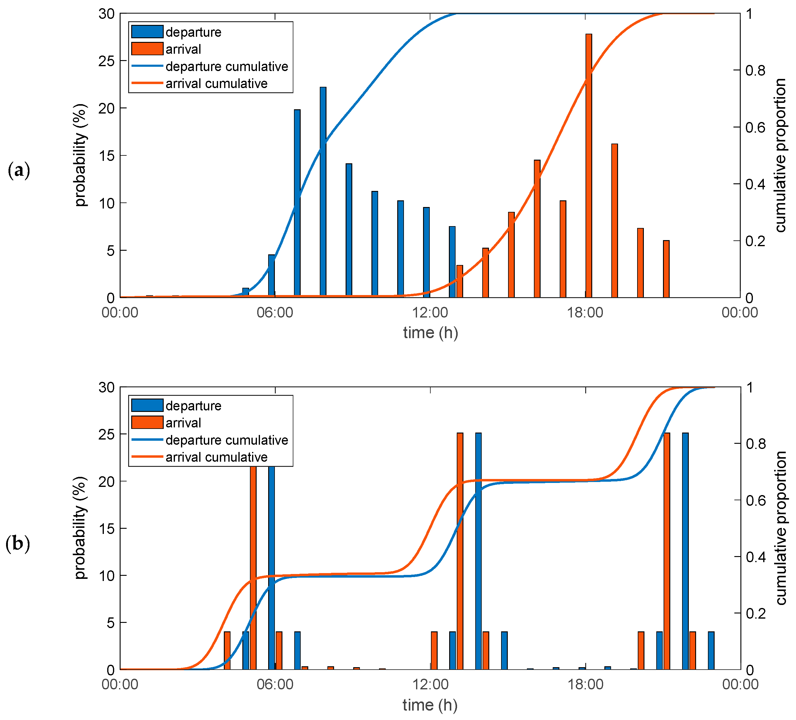
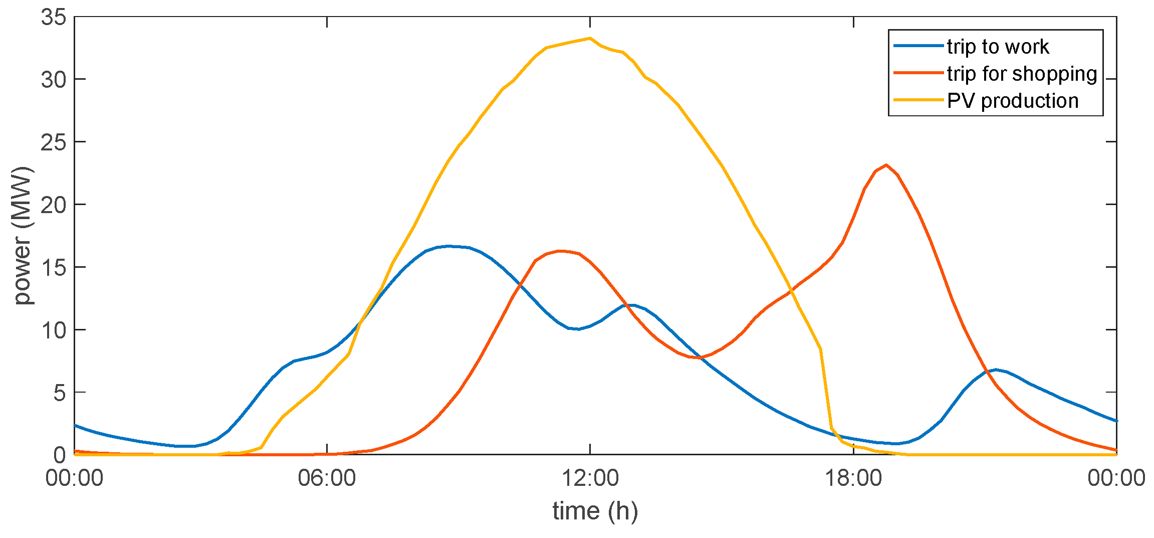
2.2. Traffic Analysis, Mobility Pattern and Traffic Model

Traffic analysis enables firstly the identification of potential locations and their respective connection points to the power grid of charging stations. They provide secondly information for the energy demand at these charging stations, which can be derived based on vehicles driving distances. In addition, they provide the necessary data for modelling synthetic charging load profiles for e-mobility.

The identification of potential locations for charging stations is based on the so-called traffic demand. To support the identification of potential locations, two basic parameters are defined: the number of motor vehicles at one location and the duration of stay at the location. In addition to the analysis of the mobility behaviour of people (individual person-related consideration), the field of traffic planning also deals with the location-related calculation of traffic volumes.

Traffic is caused by the fact that people travel to different locations in order to pursue certain activities. These activities can be summed up for the “purpose of the stay” of the people on site. The required change of location is assigned to the “purpose of stay”, also called user group. Therefore, the traffic analysis differs between seven various user groups: a trip home, a trip to work with a private or company car, a trip for shopping, a trip for execution (e.g., visit to the doctor), a trip to leisure activities and a trip to education. [23,24,25]

The mobility pattern of each user group includes original destination matrices according to Bosserhoff [23]. These matrices describe the relative proportion of arriving and departing vehicles in each hour of the day in relation to the total amount of vehicles of one day (24 h). Finally, cumulative distribution functions of arriving and departing vehicles are generated for these daily distributions. Two examples of original daily distributions according to Bosserhoff for the purpose “trip home” and “trip to work-shift operation” as well as the respective cumulative distributions are shown in Figure 1 [11]. Furthermore, by using the daily distributions of arrivals and departures, as step 1, relative distributions of the present vehicles can be derived for every hour: from the vehicles present at the beginning of an hour, the departing vehicles are added and the departing vehicles are subtracted. In step 2, the average duration of stay at the considered location will be calculated. From the daily distribution of the vehicles present, the sum of the duration of stay of all vehicles can be calculated. This sum divided by the number of arrived vehicles gives the average duration of stay per vehicle.

The distances travelled are needed for the charging station design (number of charging points, charging power) as well as for the determination of the energy demand. They are the result of the individual behaviour of persons (choice of destination) and the distance between the locations. This means that they cannot be derived directly from the location-related information. Therefore, surveys on mobility behaviour are carried out to obtain such average data like the distance travelled. Such surveys usually deal with the mobility behaviour of the inhabitants of a geographical unit (municipality, city, etc.). While the private sector is well represented in such surveys, commercial traffic is not treated so intensively. In addition, the commercial traffic differs very clearly between the various sectors. A determination of the distances travelled for commercial traffic is made possible by the evaluation of sector-specific “driving profiles” [24]. While the consideration of “driving profiles” is especially important for commercial traffic, as this is the only way to describe its characteristics and dimensions, this is of negligible interest in the private sector for an average working day. This is due to the fact that in the private sector there are usually fixed residences and thus trip purposes, for example “living - working - shopping – living”. Such trip chains are used in this paper to illustrate charging at workplaces.

In traffic modelling, the division of an area usually takes place in smaller geographical units, so-called traffic cells. The formation of traffic cells is geographically based on contiguous road network sections and administrative borders. Traffic cells combine several (postal) addresses into one larger unit. In a traffic model, the traffic between the cells (and not within the cells) is essentially calculated. Since the boundaries of the traffic cells do not necessarily match with those of the energy cells, which are created during the development of the simplified cell-based grid model, an approach had to be found to transfer the information from the traffic cells into the energy cells. For this approach, the “grid point’s method” is used in this work. Grid point data are available in Austria in the smallest unit in a 100 by 100 meter square. For the case study Leoben, the traffic model is therefore built based on this 100 by 100 meter grid unit. The cell boundaries of the energy cells can therefore be defined taking into account the grid topology and the guidelines described in [11] to achieve the best possible accuracy of the cell-based grid model. As shown in Figure 2, each grid unit has a grid point, in which the statistical data such as number of trips, average duration of stay and average distance travelled are stored for the seven various user groups. A more detailed breakdown of the data can be found in Appendix A. All data is created for each hour of the day in an average weekday. The grid units enable each energy cell to incorporate the specific grid points within its boundaries, with the result that the statistical data and the resulting traffic data can be clearly allocated to the energy cells. All grid points within an energy cell are finally aggregated to an energy node.

However, the statistics stored in the grid points do not fully cover the need for data to determine the energy demand for charging. The missing data is supplemented by comprehensive reports on mobility behaviour, such as “Österreich unterwegs 2013/2014” [25] and “Mobilität in Deutschland” [26].

In addition to the traffic analyses and mobility patterns, vehicle-related specifications such as battery capacity, average energy consumption and charging efficiency are required to model the synthetic charging load profiles for e-mobility. Therefore, based on the EV-models registered in Germany [27], 15 different EV models for passenger traffic are identified and a distribution function of the EV type is derived. An overview of the considered 15 different EV models is given in Appendix B,

Table A2. Overview of the 15 different considered EV types.

Brand of Car	Model	Battery Capacity [28] (kWh)	Average Energy Consumption [28] (kWh/100 km)
Audi	E-tron	95.0	23.7
BMW	i3	27.2	18.4
Hyundai	Ioniq Elektro	28.0	14.7
Hyundai	Kona	64.0	19.5
Nissan	e-NV 200	40.0	28.1
Nissan	Leaf	40.0	22.1
Renault	Zoe	41.0	20.3
VW	e-Golf	34.9	17.3
VW	e-up!	18.7	17.7
Jaguar	I-PACE	90.0	27.6
Kia	Soul EV	27.0	19.1
Smart	fortwo	17.6	18.3
Smart	forfour	17.6	18.3
Tesla	Model S	90.0	24.0
Tesla	Model 3	75.0	20.9

. Subsequently, the specific vehicle parameters mentioned above are assigned to each EV type based on the ADAC eco-test [28]. The specified average energy consumption is defined for an ambient temperature of 20 °C [29]. In order to take into account the seasonal variations in temperature and average energy consumption, the average energy consumption for the seasons are calculated based on average ambient temperatures for summer, winter and transition [30].

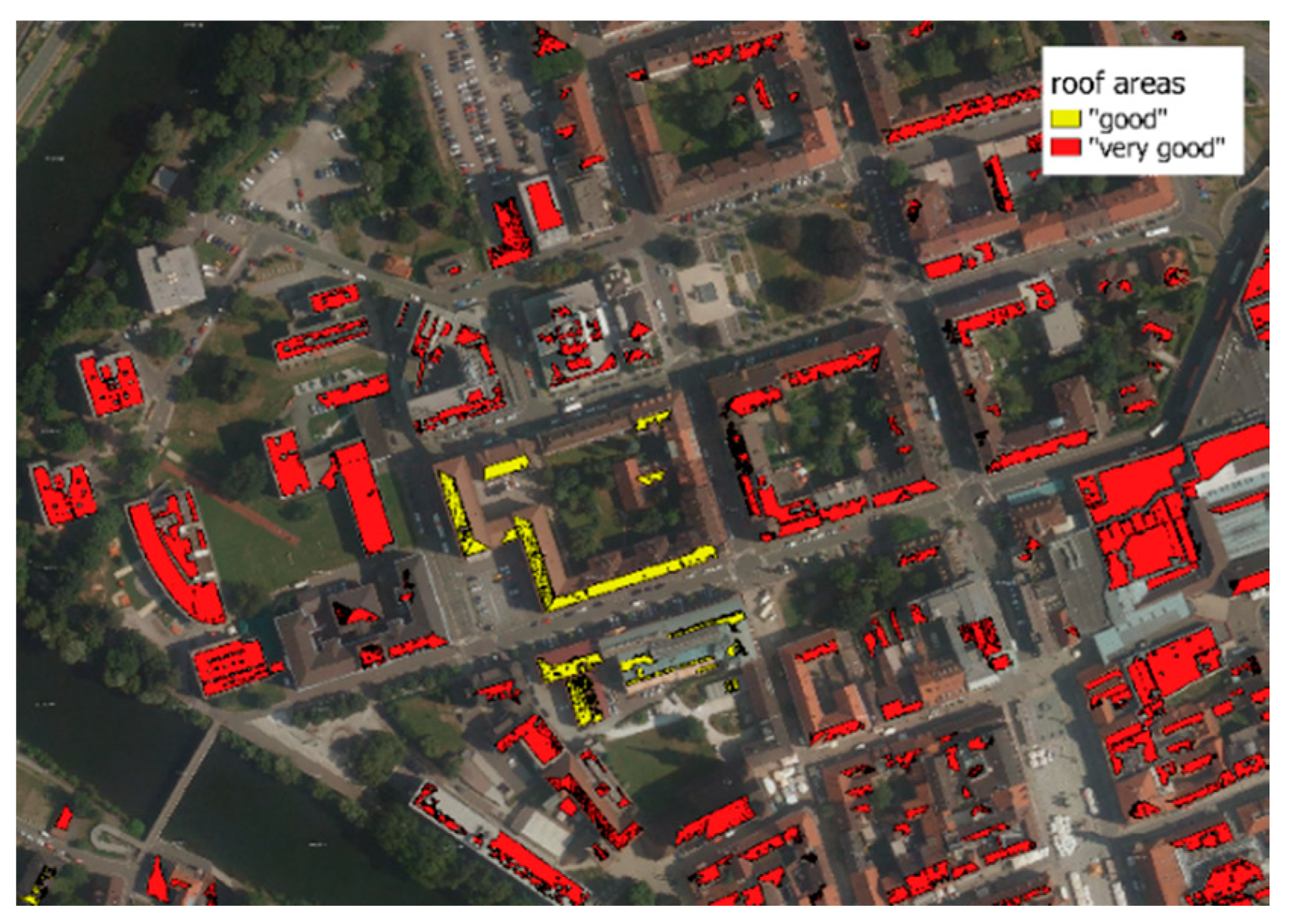
2.3. PV Potential Profiles

To determine the production profiles of the PV potentials, we use irradiation and temperature data from 2014 of the Austrian Central Institute for Meteorology and Geodynamics (ZAMG) [14] in combination with the area of suitable roofs we gained from the Styrian solar roof register from the regional government of Styria [15]. The Styrian solar roof register contains all roof areas that are suitable for the generation of solar energy and exceed a size of 20 m². Based on Airborne laser scanning (ALS) the suitable roof areas were identified and divided into “good” and “very good” areas as shown in Figure 3. The division into “good” and “very good” suitable roof areas is carried out during the data collection of the solar roof register and takes into account the size, azimuth, tilt and shading of the roof areas [31]. For each suitable roof area, detailed information such as the area in m² and the potential annual production in kWh is available in addition to the geographical location.

3. Methods

The basis of the presented case study is a simplified cell-based grid model. Therefore, the methodology used for model development is explained below. This is followed by a description of the determination and grid-implementation of time-resolved load profiles, e.g., for households, as well as for the production profiles of already existent plants (hydroelectric power, biomass cogeneration and PV, as already mentioned in Section 2.1). We also explain the determination of the synthetic charging load profiles for e-mobility and the profiles of the PV potentials in this section. Furthermore, the necessary steps for the evaluation of the grid-side effects and the energy analyses are presented. Finally, we describe the scenarios we investigate during the case study.

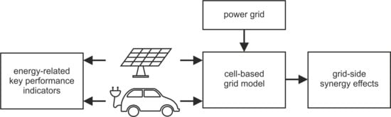
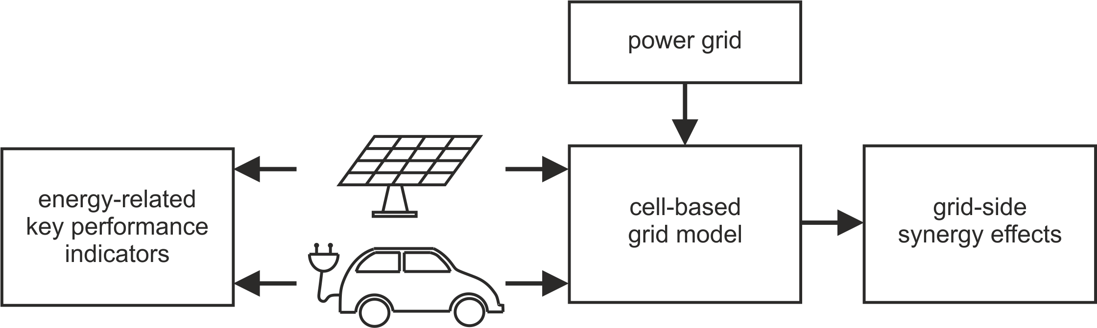
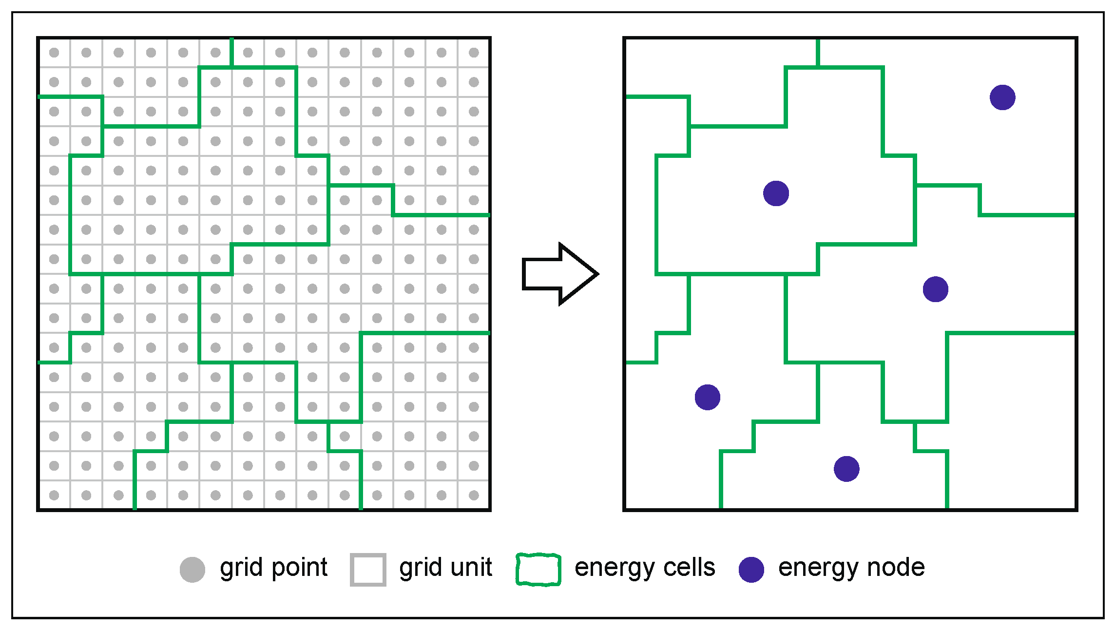
3.1. Cell-based Grid Model

The simplified cell-based grid model presented here is developed in five steps as shown in Figure 4: (i) cell classification, (ii) cell allocation, (iii) energy aggregation, (iv) development of the grid model and (v) accuracy check. If a grid model containing several voltage levels is to be developed, steps 2 to 4 must be repeated for each voltage level [11].

In step 1, the original medium-voltage grid is divided into energy cells, considering the grid topology and the topography of the depicted area. As already mentioned in Section 2.1, the cell boundaries of these cells are adapted to the grid units of the traffic analysis. In step 2, the electrical equipment (transformers, lines, grid nodes, busbars, etc.), the consumers and producers are allocated to the individual energy cells. In step 3, the assigned annual energy consumption of the consumers and annual energy production of the producers within an energy cell are aggregated into a fictitious energy node, representing virtual busbars. This aggregation is performed separately for the respective categories of standard load profiles from the BDEW [20] and the synthetic load profiles from the e-control [21]. In step 4, the simplified cell-based grid model is generated by using the software NEPLAN 5.5.6 [19]. For this, a busbar is inserted into the grid model for each energy node. After the implementation of the electrical equipment, it is connected to the energy node. Subsequently, the energy nodes are connected according to the grid topology of the original medium-voltage grid. This connects those cells with each other that enable energy export or import beyond their cell boundaries. Lines within a cell in the original medium-voltage grid structure are taken into account by implementing E-RLC modules in the grid model. In step 5, the accuracy is checked by comparison of the load flows of the simplified cell-based grid model with those of the original medium-voltage grid. We describe this approach of grid simplification in detail in [11].

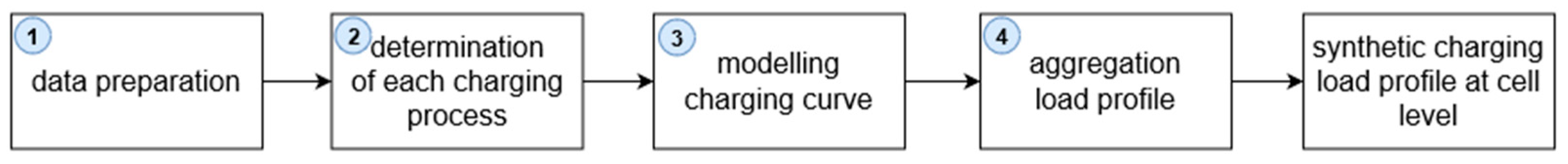
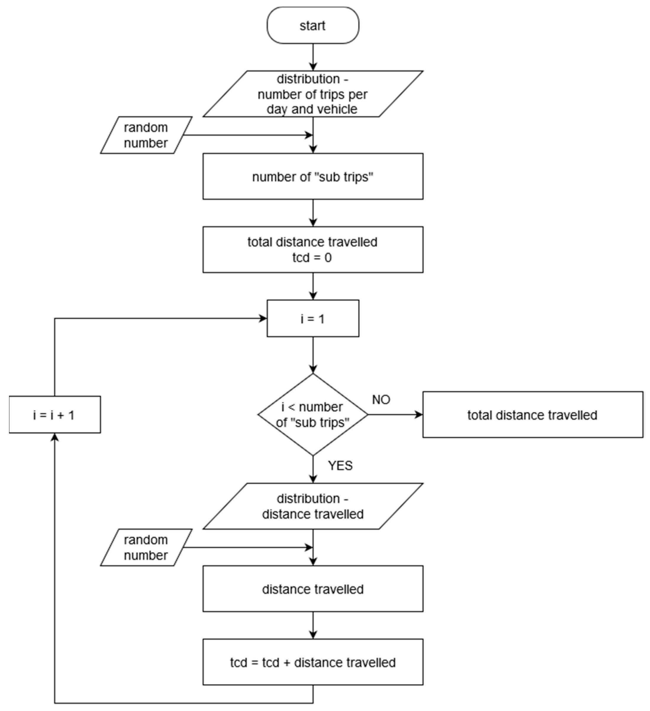
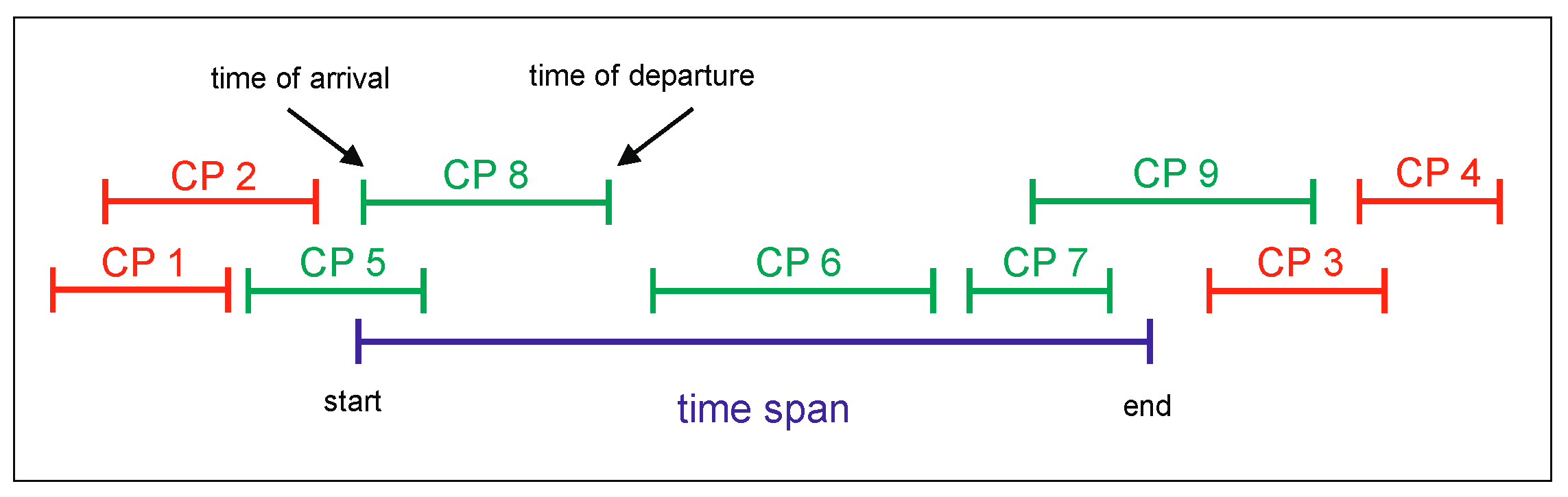
3.2. Determination Load and Production Profiles

Following the model development, annual time-resolved (15-min mean values) load and production profiles are modelled for the aggregated annual energy consumption and production. Therefore, we use the standard load profiles from the BDEW [20] and the synthetic load profiles from the e-control [21]. These profiles represent normalised load profiles for categories like household, commercial, agricultural, interruptible power supplies, and public lighting. Based on these normalised profiles (1000 kW/a), we calculate the time-resolved annual load profiles.

For the determination of the synthetic charging load profiles for the e-mobility we apply as shown in Figure 5, four steps: (i) data preparation, (ii) determination of each charging process, (iii) modelling charging curve and (iv) aggregation of the load profiles [11].

In step 1, the traffic grid points and the mobility behaviour presented in Section 2.2 are prepared for the further procedure. In addition to the aggregation of all grid points and the data contained therein (e.g., number of trips) within a cell, this includes the preparation of the distribution functions (arrival/departure/EV type), already mentioned in Section 2.2. Based on the average distances travelled at grid point level, a distribution function for the distance travelled per user group and cell is derived by aggregating all distances travelled within a cell. In step 2, each charging process (CP) within a user group and cell is determined based on the distribution functions by applying probabilistic approaches and the selected charging strategy (e.g., uncontrolled/controlled charging). Each charging process is described by time of arrival, time of departure, EV type and distance travelled. The number of charging processes per cell and user group on a weekday is derived from the aggregation of grid points performed in step 1. Based on the number of trips per weekday, empirical factors from statistical data are used to determine the number of trips for Saturday and Sunday for each user group and cell. The number of trips per day corresponds to today’s mobility behaviour. A change in mobility behaviour is difficult to estimate according to traffic planners, therefore it is not taken into account. Hence, we assume that in a scenario with an EV penetration of 100%, each distance travelled represents a trip with an electric vehicle. In step 3, the charging curve for each charging process is modelled according to the state-of-the-art constant current (CC) – constant voltage (CV) charging process. In step 4, all charging processes within a cell are aggregated to a synthetic charging load profile. We describe the general procedure of determining synthetic cell-based charging load profiles for electric vehicles in detail in [11].

For this work we have expanded the method we have described in [11]: Firstly to consider only selected user groups like “trip to work with a private car” for modelling the synthetic charging load profiles. Secondly to enable “intelligent controlled charging”, called charging strategy 2.

The extension regarding the selection of the considered user groups consists of creating a trip chain for the selected user groups, which takes place in step 2. The creation of such a trip chain is necessary because the selection of user groups means that there is no longer a charging process after each trip. Therefore, the trips of the non-selected user groups are cumulated into the selected ones, so that the distances travelled by the non-selected user groups can be considered. For this purpose, a trip of the selected user groups consists of several “sub trips”, e.g., the trip chain: “working - living - shopping - working” of the user group “trip to work with a private car” consists of three “sub-steps”. For each trip of the selected user groups resulting from step 1, the total distance travelled is determined as shown in Figure 6. For this, the number of “sub trips” is defined by applying the probabilistic approach to the statistical distribution of the number of trips made per day and vehicle. Subsequently, the distances travelled are determined for each “sub trip” and summed up, so that the charging curve is modelled, based on the total distance travelled.

The introduction of charging strategy 2, “intelligent controlled charging”, also takes place in step 2.

Table 1. Comparison of charging strategy 1 and charging strategy 2.

Charging Strategy	Type of Charging	Start of the Charging Process (CP)	Further Information
1	Uncontrolled	Time of arrival	Basis for charging strategy 2
2	Intelligent controlled	Depending on the time span in which the CP can be shifted	Two approaches: Shifting CPs into PV Peak or sequencing of CPs

shows the comparison of charging strategy 1 and 2: As shown, in charging strategy 1 the arrival of the EV starts the charging process, while in charging strategy 2, a time shift of the start of the charging process is considered.

The charging strategy 2 takes into account two different approaches, which depend on the mobility behaviour. For each peak in the synthetic charging load profile, a time span is defined in which the charging processes can be shifted depending on the occurrence (morning, midday, afternoon, evening) of the peak. Charging processes which occur during the morning and midday peak are shifted into the peak of the PV production. For the charging processes that take place during the afternoon and evening peaks, the aim is to reduce the charging load by sequencing the charging processes with the boundary condition that the EVs are fully charged in the morning. This does not involve a reduction of the charging power of the individual charging process.

The defined time span is used to decide for each charging process whether it can be shifted or not, see Figure 7. As a generic example, it is not possible to shift the charging processes CP 1 to CP 4 (red) into the time span, because their time of arrival and their time of departure are before or after the defined time span. This means that this charging process takes place at the original time as defined in charging strategy 1. In principle, the charging processes CP 5 to CP 9 can be shifted into or within the time span. During the shifting and sequencing of the charging process, it must be ensured that this is only possible within the duration of stay of the EV, with the boundary condition that the EV is fully charged at the time of departure. For example, if charging process CP5 is shifted to the start of the time span and the remaining time is not sufficient for a fully charged EV, the charging process will also take place at the original time as defined in charging strategy 1.

Following the identification of those charging processes that can be shifted into or within the time span, the shifting or sequencing of these charging processes is carried out according to defined criteria. These criteria represent the duration of stay, a priority factor, start of the charging process and the duration of the charging process. The priority factor describes the ratio between duration of stay and duration of the charging process. This means that the closer this ratio is to one, the shorter the period of time in which this charging process can be shifted within the duration of the vehicle’s stay. Such charging processes are assigned with new starts of the charging process as soon as possible. Within the framework of this charging strategy, only the start of the charging processes is changed. All other data (e.g., EV type, charging power, distance travelled) for modelling the charging curves remain unchanged. Therefore, after applying charging strategy 2, the methodology described above can be continued in step 3.

3.3. Determination of PV Potential Profiles

The modelling of the PV potential profiles is based on an irradiation model according to Perez et al. [32,33,34], which is described in more detail in Duffie et al. [35] and Pretschuh et al. [36]. Based on the irradiation and temperature data as well as data from the described solar roof register, the model calculates the direct and diffuse share of the radiation on the inclined surface and converts it into electricity. As a result, annual time resolved PV potential profiles are generated for each cell, which take into account seasonal conditions based on real irradiation and temperature data. A penetration of 100% PV potential requires that all potential roof areas classified as “good” and “very good” in the solar roof register are considered during the determination of the PV potential profiles.

3.4. Simulation, Calculation and Evaluation

To analyse the grid-side synergy effects between e-mobility and PV potentials, load flow calculations with annual load profiles (15-min mean values) are performed for different scenarios. These scenarios differ between the penetration of EV, the penetration of PV, charging power and charging strategy (controlled and uncontrolled charging). The results from the load flow calculations are analysed with regard to the utilisation of the equipment (e.g., transformer, lines). This is followed by the identification of overloaded equipment, the percentage value, the duration and time of occurrence of these overloads and thus the identification of worst-case weeks. In addition, the influence of PV and EV interactions on these overloads is investigated. Besides the grid-side synergy effects, energy-based analyses are carried out for the same scenarios. For this purpose, the following four key performance indicators are defined: (i) the residual load $P_{Res}$, (ii) the degree of self-generation (DSG), (iii) the degree of self-sufficiency (DSS) and (iv) the self-consumption ratio (SCR). The residual load describes the difference between the power of consumers and e-mobility $P_{Consumer+EV}$ and the power of the photovoltaic potential $P_{PV}$. If in a certain 15-min time step the PV production exceeds the total load, the residual load becomes negative and vice versa.

$$P_{Res}=P_{Consumer+EV}-P_{PV}$$

(1)

While the residual load is determined for each 15-min time step of the annual total load profile and the annual PV potential profile, the defined time frame for the determination of DSG, DSS and SCR is defined as one day (96 15-min time steps). The calculation of daily values, in comparison to the determination of an annual value, enables the seasonal consideration of the interaction between the e-mobility and PV potentials.

To explain the DSG, DSS and SCR, Figure 8 shows a generic load profile (consumer and EV) and a generic PV production profile as an example.

The degree of self-generation (DSG) describes the locally produced energy in relation to the locally consumed energy for a defined time frame:

$$DSG=\frac{E_{PV}}{E_{Consumer+EV}}=\frac{{{\displaystyle \int }}_{t_{start}}^{t_{end}}(P_{PV}\left(t\right)) dt}{{{\displaystyle \int }}_{t_{start}}^{t_{end}}(P_{Consumer+EV}\left(t\right)) dt}$$

(2)

where $E_{PV}$ is the total locally produced energy and $E_{Consumer+EV}$ is total energy demand for the defined time frame.

The degree of self-sufficiency (DSS) considers the ratio between the directly consumed part of the locally produced energy $E_{SC}$ and the total energy demand. This means that this criterion describes the proportion of the total load required that can be covered directly by the PV potential:

$$DSS=\frac{E_{SC}}{E_{Consumer+EV}}=\frac{{{\displaystyle \int }}_{t_{start}}^{t_{end}}(\min \{P_{Consumer+EV}\left(t\right), P_{PV}\left(t\right)\}) dt}{{{\displaystyle \int }}_{t_{start}}^{t_{end}}(P_{Consumer+EV}\left(t\right)) dt}$$

(3)

The self-consumption ratio (SCR) relates the directly consumed part of the locally produced energy to the total locally produced energy:

$$SCR=\frac{E_{SC}}{E_{PV}}=\frac{{{\displaystyle \int }}_{t_{start}}^{t_{end}}(\min \{P_{Consumer+EV}\left(t\right), P_{PV}\left(t\right)\}) dt}{{{\displaystyle \int }}_{t_{start}}^{t_{end}}(P_{PV}\left(t\right)) dt}$$

(4)

3.5. Scenario Definition

To identify which of the seven user groups from the traffic analyses are particularly relevant for the investigation of the synergy effects between e-mobility and PV potential, the potential for the direct use of PV production per user group is examined. For the case study presented here, the user groups “trip for shopping”, “trip for execution” and “trip to work” have the highest energy demand in relation to the total energy demand of e-mobility based on the traffic analysis. Since the user groups “trip for shopping” and “trip for execution” have the same characteristic load profile, only the user groups “trip for shopping” and “trip to work” are shown as examples in Figure 9. The figure is used to visualize the determination of the potential for the direct use of PV production for the user groups “trip for shopping” and “trip to work”. For the user group “trip to work”, the user groups “trip to work with a private car” and “trip to work with a company car” are aggregated due to their similar behaviour. The characteristic of the synthetic charging load profile for the user group “trip to work” is strongly dependent on the sector-specific jobs within the considered area. Therefore, the evening peak, which occurs due to an existing shift operation, can be omitted when looking at another area. The number of peaks for the user group “trip for shopping” is independent of the area under investigation. This means that as soon as there are shopping facilities in the area under consideration, and thus a shopping user group exists, a peak at noon and in the afternoon or evening occurs. In the example shown, around 80% of the energy demand of the user group “trip to work” can be directly covered by PV production, while only 60% can be directly supplied for the user group “trip for shopping”.

The analysis of all user groups indicates that with an increasing number of charging processes during the day, the direct use of the PV production increases and thus the potential. Based on the user behaviour and the share of PV use, the user group “trip to work” can be identified as the user group with the highest potential. Therefore, we have focused on the user groups “trip to work with a private car” and “trip to work with a company car” in combination with a trip chain model to investigate the synergy effects between e-mobility and PV potentials in the case study presented here. Using the trip chain model, the charging energy of the other five user groups is accumulated into these two user groups. Since the number of weekend trips for these user groups is decreasing significantly and it should be ensured that all distances travelled at the weekend are also taken into account, the user group “trip home” is also considered at the weekend.

As already mentioned, the scenarios differ among each other in the penetration of EV and PV. For this purpose, the penetration of EV and PV is varied by 0%, 20%, 40%, 60%, 80% and 100% respectively. In a scenario, all cells have always the same penetration of EV and PV, this means for example that all cells have a penetration of 20% PV and a penetration of 80% EV. This assumption was made, because there are no statistical distributions for urban areas that allow an individual penetration for each cell. Furthermore, two different charging powers (3.7 kW and 11 kW) are considered. For both charging powers, a distinction is made between charging strategy 1 (uncontrolled charging) and charging strategy 2 (controlled charging).

The reference scenario describes the status quo (without PV Potential and future e-mobility) of the medium-voltage grid to be examined. The overview of all simulated scenarios is given in Appendix B,

Table A1. Overview of all simulated scenarios during the presented case study.

Penetration (%)		CP (kW)	CS	Penetration (%)		CP (kW)	CS	Penetration (%)		CP (kW)	CS	Penetration (%)		CP (kW)	CS
PV	EV			PV	EV			PV	EV			PV	EV
0	0*	0	0
0	20	3.7	1	0	20	11	1	0	20	3.7	2	0	20	11	2
0	40	3.7	1	0	40	11	1	0	40	3.7	2	0	40	11	2
0	60	3.7	1	0	60	11	1	0	60	3.7	2	0	60	11	2
0	80	3.7	1	0	80	11	1	0	80	3.7	2	0	80	11	2
0	100	3.7	1	0	100	11	1	0	100	3.7	2	0	100	11	2
20	0*	0	0
20	20	3.7	1	20	20	11	1	20	20	3.7	2	20	20	11	2
20	40	3.7	1	20	40	11	1	20	40	3.7	2	20	40	11	2
20	60	3.7	1	20	60	11	1	20	60	3.7	2	20	60	11	2
20	80	3.7	1	20	80	11	1	20	80	3.7	2	20	80	11	2
20	100	3.7	1	20	100	11	1	20	100	3.7	2	20	100	11	2
40	0	3.7	1	40	0	11	1	40	0	3.7	2	40	0	11	2
40	20	3.7	1	40	20	11	1	40	20	3.7	2	40	20	11	2
40	40	3.7	1	40	40	11	1	40	40	3.7	2	40	40	11	2
40	60	3.7	1	40	60	11	1	40	60	3.7	2	40	60	11	2
40	80	3.7	1	40	80	11	1	40	80	3.7	2	40	80	11	2
40	100	3.7	1	40	100	11	1	40	100	3.7	2	40	100	11	2
60	0*	0	0
60	20	3.7	1	60	20	11	1	60	20	3.7	2	60	20	11	2
60	40	3.7	1	60	40	11	1	60	40	3.7	2	60	40	11	2
60	60	3.7	1	60	60	11	1	60	60	3.7	2	60	60	11	2
60	80	3.7	1	60	80	11	1	60	80	3.7	2	60	80	11	2
60	100	3.7	1	60	100	11	1	60	100	3.7	2	60	100	11	2
80	0	0	0
80	20	3.7	1	80	20	11	1	80	20	3.7	2	80	20	11	2
80	40	3.7	1	80	40	11	1	80	40	3.7	2	80	40	11	2
80	60	3.7	1	80	60	11	1	80	60	3.7	2	80	60	11	2
80	80	3.7	1	80	80	11	1	80	80	3.7	2	80	80	11	2
80	100	3.7	1	80	100	11	1	80	100	3.7	2	80	100	11	2
100	0*	0	0
100	20	3.7	1	100	20	11	1	100	20	3.7	2	100	20	11	2
100	40	3.7	1	100	40	11	1	100	40	3.7	2	100	40	11	2
100	60	3.7	1	100	60	11	1	100	60	3.7	2	100	60	11	2
100	80	3.7	1	100	80	11	1	100	80	3.7	2	100	80	11	2
100	100	3.7	1	100	100	11	1	100	100	3.7	2	100	100	11	2

CP… charging power/CS… charging strategy; 0*… Since a penetration of 0% EV only takes into account the demand for e-mobility that is already present in the status quo of the power grid, no charging power and charging strategy is assigned to these scenarios. Therefore, the simulation of scenarios with a penetration of 0% EV for different charging power and charging strategy is not necessary.

.

4. Results and Discussion

In this section the developed cell-based grid model, which forms the basis of the case study, is presented. Afterwards, the results of the load flow calculations are analysed with regard to grid-side synergy effects. Finally, the results from the energy analyses are discussed.

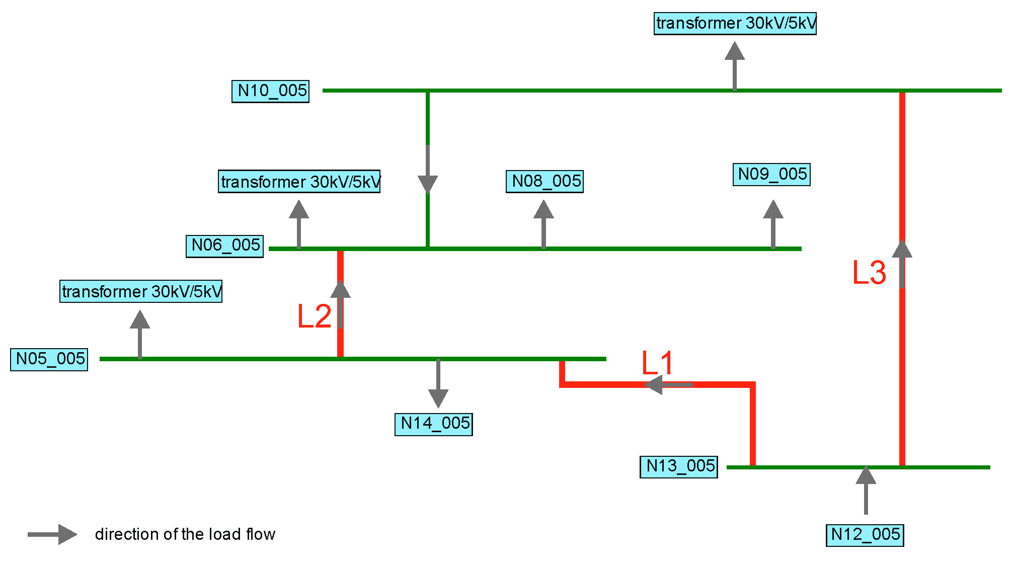
4.1. Cell-Based Grid Model

The original medium-voltage grid of the city of Leoben is divided into 26 energy cells. Figure 10 illustrates the developed simplified cell-based grid model, where the 30 kV voltage level is shown in blue and the 5 kV voltage level in green. To clearly distinguish the two voltage levels, the 30 kV level is marked with the ending _030 and the 5 kV level with the ending _005. Since the 30 kV voltage level is not designed to cover the complete area of Leoben, not every cell has a connection to the 30 kV voltage level. The 110 kV voltage level of the Leoben substation was chosen as the slack node, so that the load flows between the 30 kV and 110 kV voltage level can also be analysed. The slack node thus corresponds to the energy node N10_110. Since there are two 110 kV/30 kV transformers in the substation due to redundancy, both are also shown in the grid model.

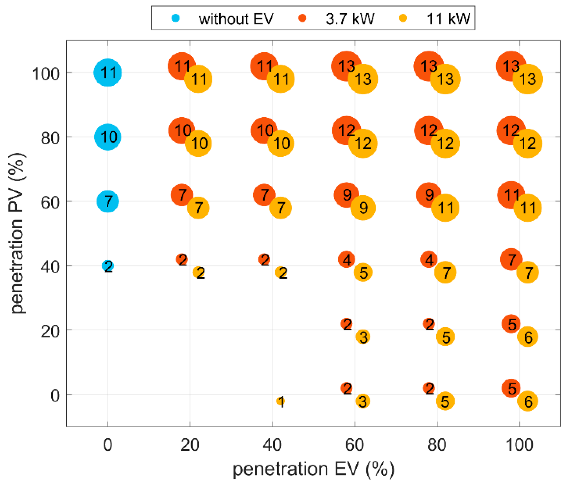
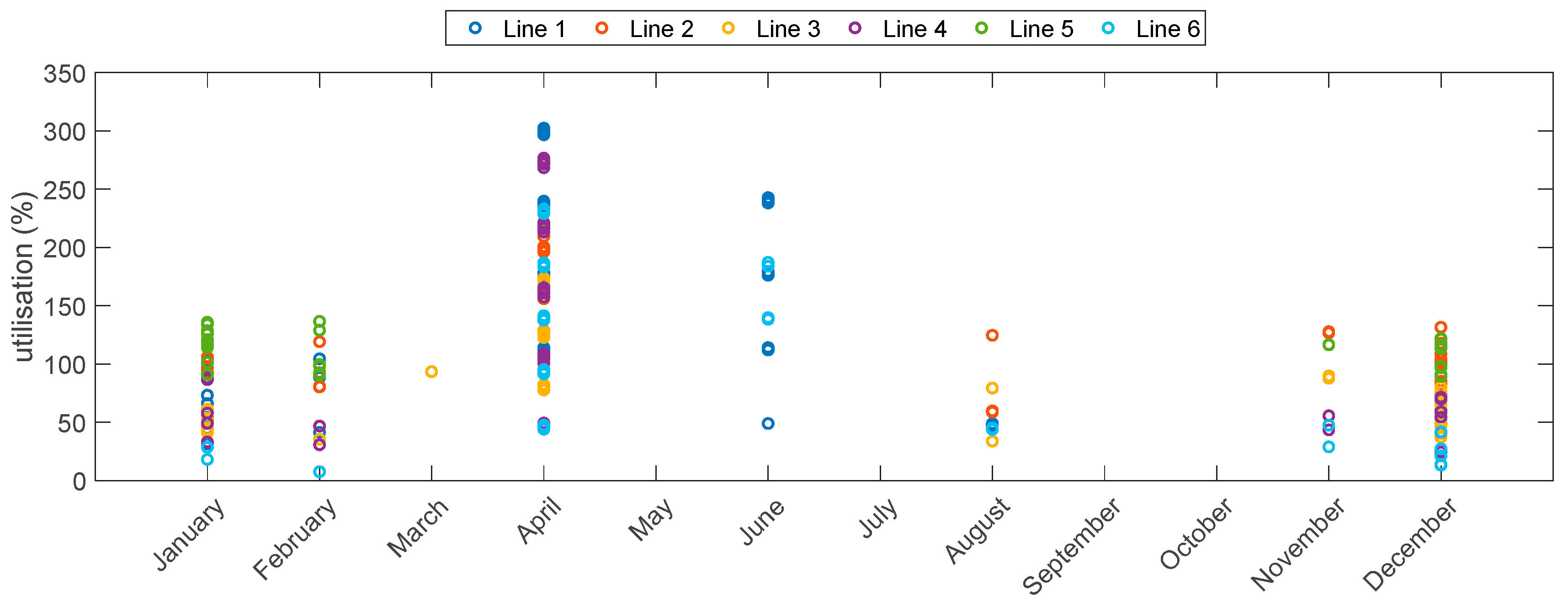
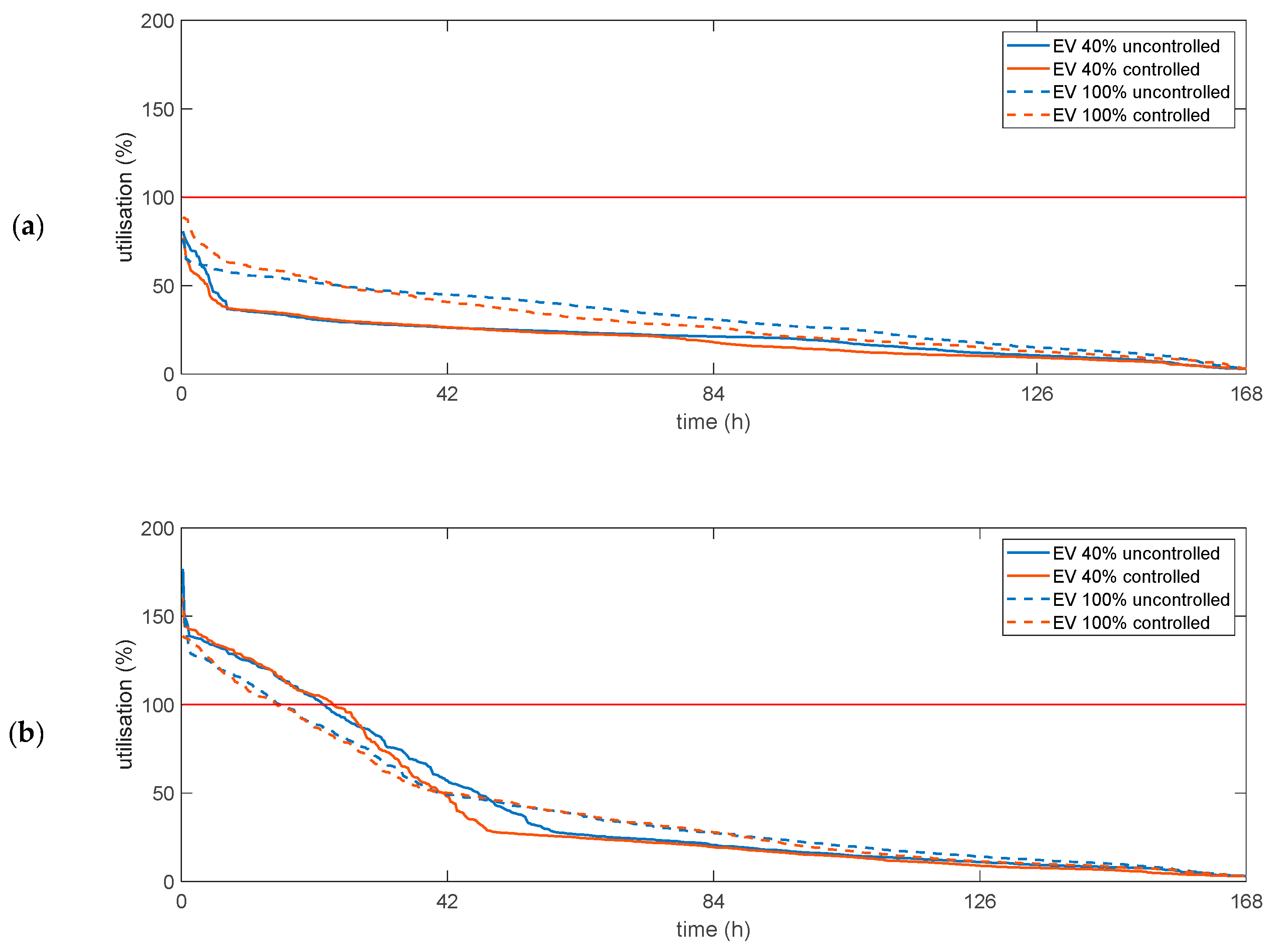
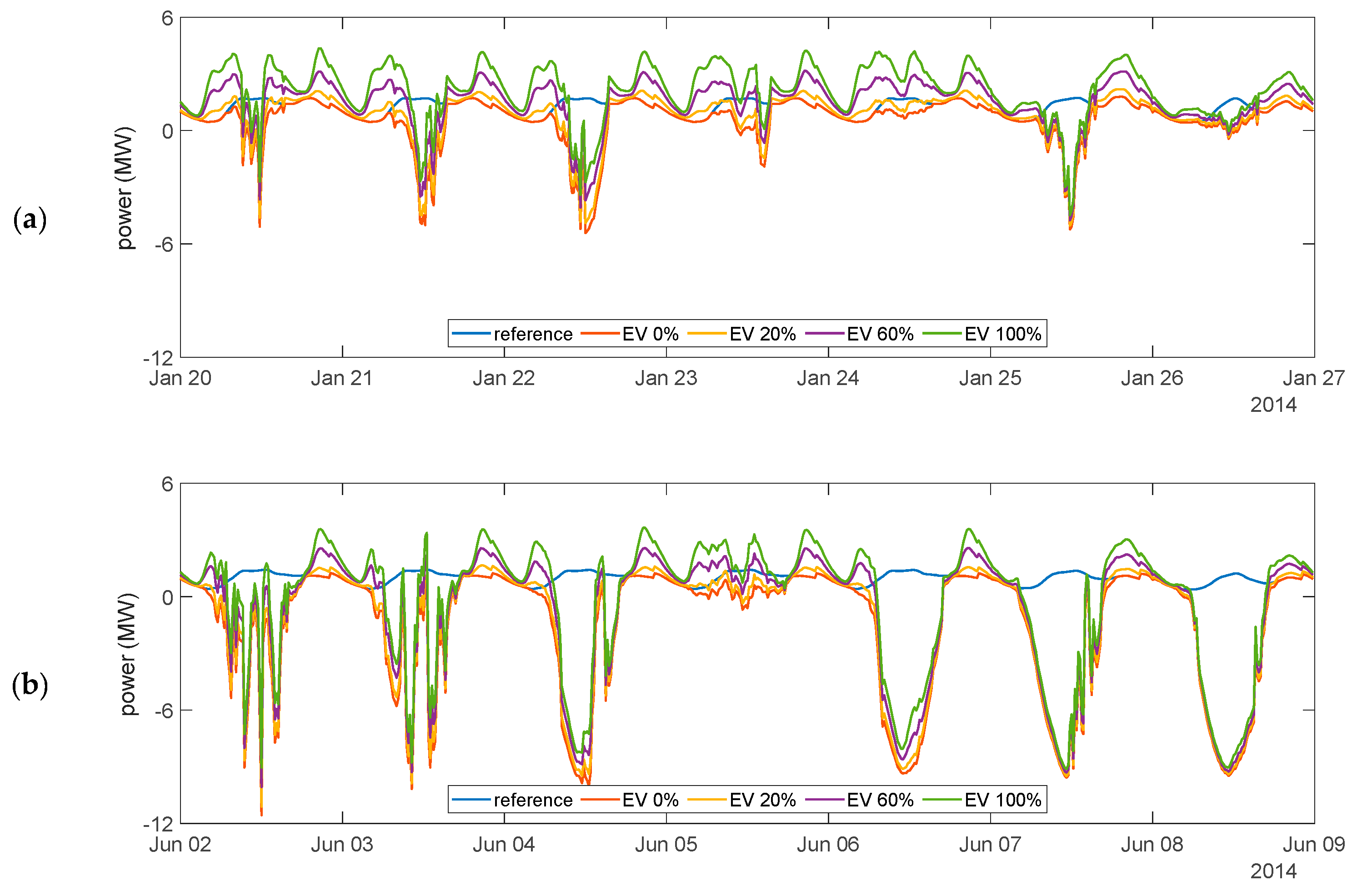
4.2. Grid-side Synergy Effects

Based on the simplified cell-based grid model and the annual load and production profiles, load flow calculations are performed for the different scenarios, described in Section 3.5. The results of the load flow calculations are analysed with regard to grid-side synergy effects between e-mobility and PV potential. The results presented here focus on the utilisation of the lines of the 5 kV voltage level.

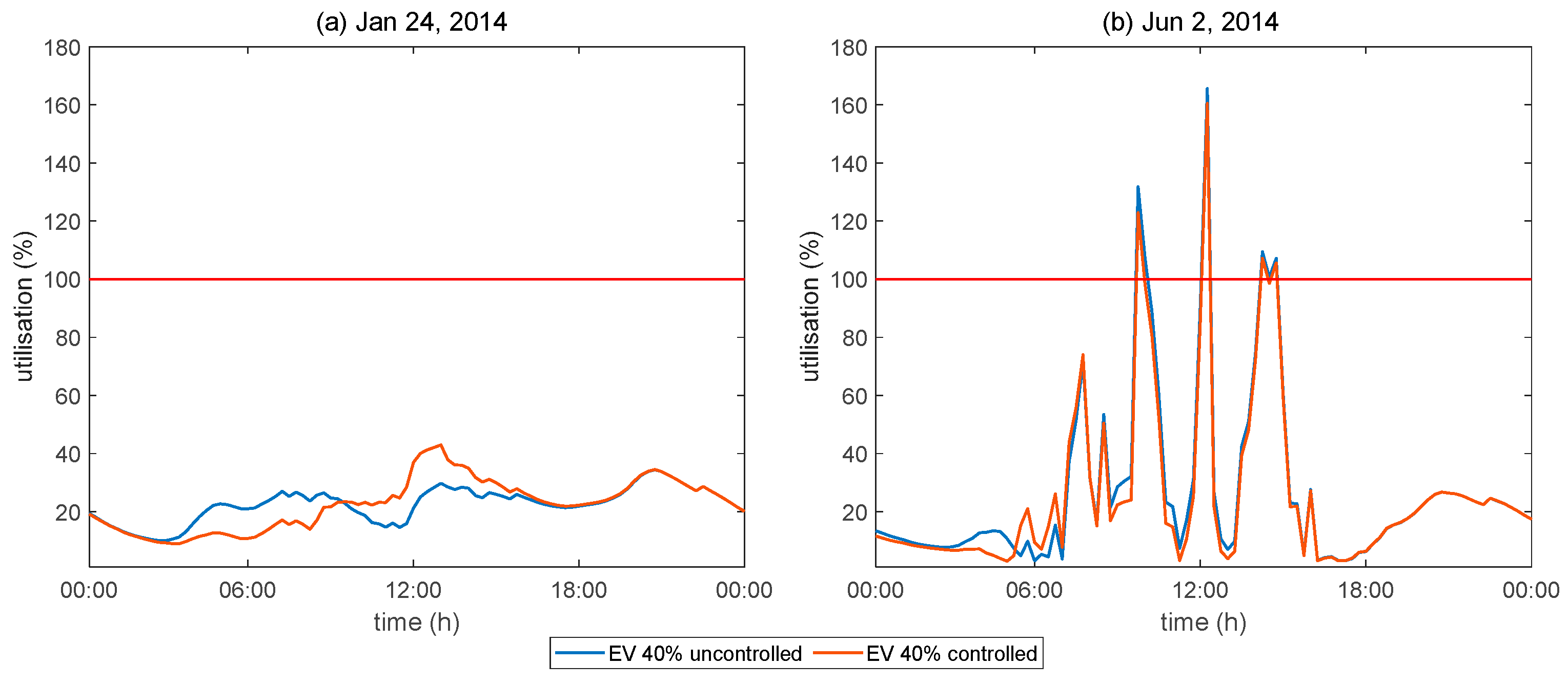
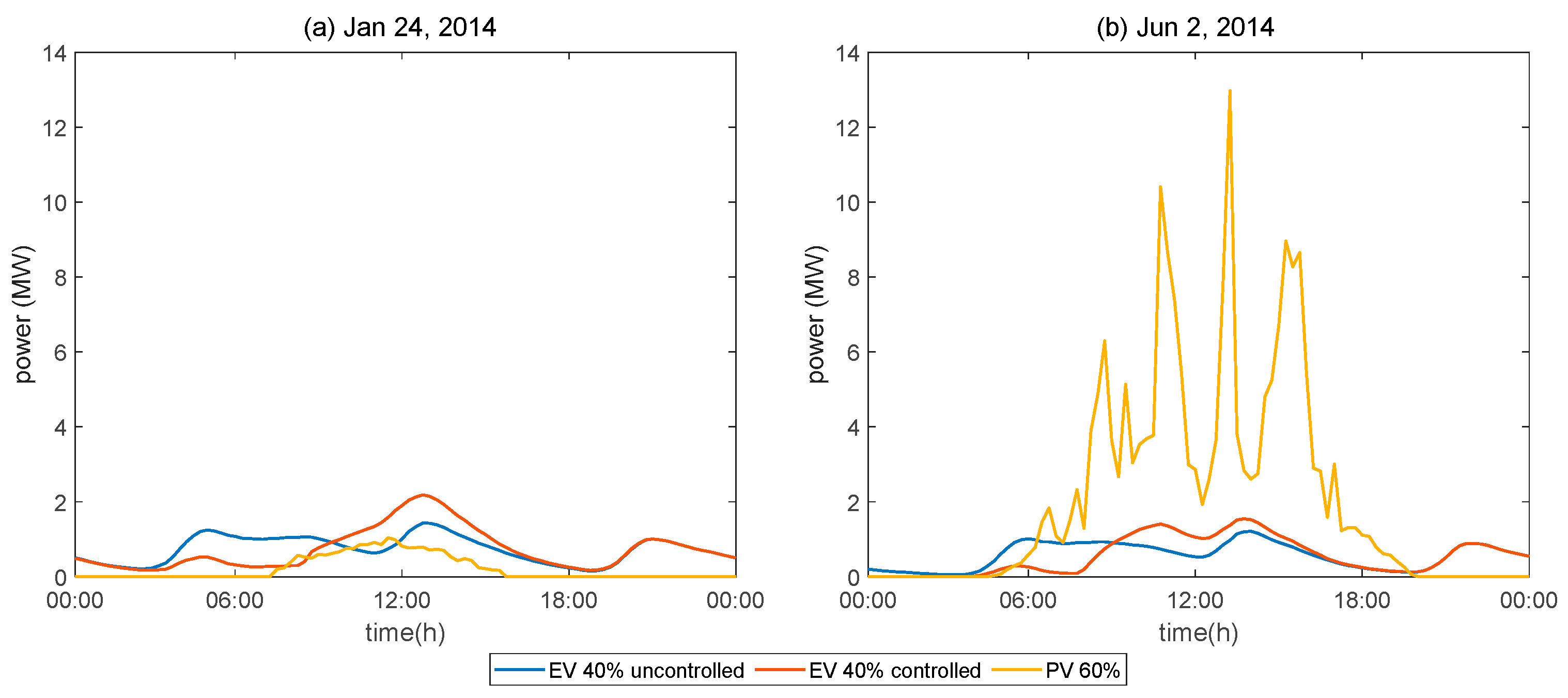
4.2.1. Charging Strategy 1 – Uncontrolled Charging

The number of overloaded lines of the 5 kV voltage level with corresponding penetration of EV and PV for the charging capacities 3.7 kW and 11 kW and charging strategy 1 is shown in Figure 11. Since a penetration of 0% EV only takes into account the demand for e-mobility that is already present in the status quo of the power grid, no additional charging power is assigned to these scenarios and they are therefore referred to as without EV. With increasing EV and PV penetration as well as charging power, the number of overloaded lines increases. The use of PV potentials without e-mobility leads to line overloads at penetration rates of 40% PV and higher. E-mobility without PV potential, too, only causes line overloads when the penetration rate is over 40% and the charging power is 11 kW. With a penetration of 20% PV, the line overload caused by a penetration of 40% EV and a charging power of 11 kW can be avoided.

In addition to the number of overloaded lines, the model also determines which lines are affected and where they are located in the power grid model and geographically. Figure 12 shows the cell division for the energy cells of the city of Leoben and the geographical location of the 13 overloaded lines, with the six most stressed lines in red. The identification of the most stressed lines is based on the maximum utilisation of the overloaded lines and the duration of the overload for all scenarios. These overloaded lines are also illustrated in Figure 10, which shows the grid plan of the cell-based grid model.

With the exception of the already mentioned avoidance of line overload at a penetration of 40% EV with a penetration of 20% PV, the different combinations of the penetrations of PV and EV do not lead to a reduction of the number of overloaded lines. Therefore, according to Figure 11 there are no obvious positive synergies between e-mobility and PV potential for charging strategy 1 for the number of overloaded lines. To investigate the interaction between e-mobility and PV potential in more detail, we determine the maximum line utilisation and the duration of overloads. For this purpose, we examine when the maximum utilisations of the lines occur and whether this is caused by the penetration of EV or PV. As illustrated for the most stressed lines in Figure 13, line overloads occur mainly in winter as well as in April and June. While the overloads in winter are due to load peaks of e-mobility, those in April and June are mainly due to production peaks of PV potentials. Furthermore, the worst-case weeks are identified based on the time of occurrence of the maximum load. Those worst-case weeks, for example, are used to compare scenarios with uncontrolled and controlled charging (charging strategy 1 vs. charging strategy 2).

Two of the six most stressed lines are selected to analyse the duration of the line overloads in detail. For this purpose, annual duration curves are modelled for each line and scenario based on the sorted utilisation of the line. While line 1 is overloaded for the first time at a penetration of 40% PV, the overload on line 5 occurs first at a penetration of 40% EV and a charging power of 11 kW. Since the duration of overload is less than 10 h for both lines, the next higher penetration of PV and EV is chosen for demonstration purposes of the interaction between e-mobility and PV potential.

Table 2. Duration of overloads (utilisation > 100%) for the lines 1 and 5 – charging power 3.7 kW and 11 kW, using charging strategy 1.

Penetration (%)		Duration of Overload (h) Line 1		Penetration (%)		Duration of Overload (h) Line 5
PV	EV	3.7 kW	11 kW	PV	EV	3.7 kW	11 kW
60	0	506.50	506.50	0	60	154.50	155.75
60	20	454.00	450.50	20	60	107.75	132.25
60	40	396.75	392.00	40	60	84.25	106.00
60	60	349.50	346.25	60	60	62.75	92.50
60	80	300.75	294.75	80	60	47.50	79.00
60	100	258.5	206.75	100	60	39.00	67.00

shows the comparison of the duration of the line overloads of lines 1 and 5 depending on the charging power. For line 1 we investigate the influence of an increasing e-mobility penetration at a fixed penetration of 60% PV. With a penetration of 60% PV and the current demand, the duration of overload is 506.5 h per year. By integrating a penetration of 100% EV, the duration of overload can be reduced to 258.5 h per year at a charging power of 3.7 kW and 206.75 h per year at a charging power of 11 kW respectively. The comparison of the duration of overloads for a penetration of 100% EV shows that at a charging power of 11 kW, the reduction in the duration of the overload is greater by around 50 h per year than at a charging capacity of 3.7 kW. This higher reduction is due to the increased power requirement of e-mobility at a charging power of 11 kW compared to 3.7 kW. As a result of this increase, the production surplus at the peak of the PV potential is reduced and thus the duration of the line overload.

However, an increased power requirement of e-mobility due to the higher charging power can also lead to an increasing grid load. This increase in grid load can be seen in Table 2 for line 5. While the duration of the line overload at a fixed penetration of 60% EV and a charging power of 3.7 kW is reduced from 154.50 h per year without PV potential to 39.00 h per year with a penetration of 100% PV, the duration of the overload at a charging power of 11 kW is reduced from 155.75 h per year only to 67.00 h per year.

The duration of the overload shown in Table 2 is graphically illustrated in Figure 14 using the sorted annual duration curves of the line utilisation for the lines 1 (a) and 5 (b) for the range 0 to 600 h at a charging power of 3.7 kW. In addition to the already described reduction of the duration of the line overload, the decrease of the utilisation can also be seen. For the shown range (0 to 600 h) of the sorted annual duration curves, the comparison of the utilisation of line 1 at a penetration of 0% EV with the utilisation at a penetration of 100% EV shows a reduction of the utilisation between 6% and 19%. For line 5, a decrease in line utilisation of up to 15% is achieved for the range of 0 to 600 h of the sorted annual duration curve with an increase in penetration from 0% PV to 100% PV.

As demonstrated by the example of the lines 1 and 5, the higher the penetration of EV with fixed penetration of PV, the lower the duration of the line overloads as well as the maximum utilisation and vice versa. The charging power also has a considerable influence on the line utilisation and thus on the overload of the lines. While a higher charging power in summer further reduces the power surplus caused by PV production and thus relieves the grid, in winter it can lead to higher and longer overloads.

In the scenarios presented here, the same penetration of EV and PV is considered for all cells, therefore in some cells large differences between PV production and the power requirements of e-mobility occur. For further reduction or possibly complete avoidance of overloads, it is necessary to find the optimal balance between PV production and the power requirements of e-mobility for each cell.

4.2.2. Charging Strategy 2—Controlled Charging

A comparison of the scenarios with charging strategy 1 and 2 based on two worst-case weeks is carried out to determine the influence of controlled charging on the grid utilisation compared to uncontrolled charging and the resulting synergy effects between e-mobility and PV potential. For this purpose, one week is in winter (20 January to 26 January) and one in summer (2 June to 8 June). The most stressed days of this week are 24 January and 2 June, respectively. The comparison of the line utilisation in Figure 15 shows for line 1 for a penetration of 40% EV and 60% PV and a charging power of 3.7 kW that controlled charging can lead to both, a reduction but also to an increase in the utilisation of the line. By applying charging strategy 2, the charging processes during the day are shifted into the peak of the PV production; thereby an increase of the power requirement of e-mobility can occur within the period of the peak of the PV potentials as shown in Figure 16.

This increase in power demand leads to an increased line utilisation if the PV potential is not sufficient, as demonstrated in Figure 15a for the 24 January. On 2 June the PV potential is significantly higher than the power demand from EV (see Figure 16b), which means that the line utilisation can be reduced at noon. As shown in Figure 15b, however, it is by far not possible to avoid the overloads. The difference of about 12 MW between the maximum peak value of the PV production on the 2 June and that on the 24 January, shown in Figure 16, does not allow any conclusions concerning other days and their maximum peak values due to the PV potentials modelled in dependence on irradiation and temperature data.

The utilisation of line 1 cannot be directly compared with the difference between the EV charging load and the PV potential of cell 13 (Figure 16). On the one hand, the utilisation of the line depends on the balance of the total demand (e-mobility and other consumption) as well as the PV potential and the resulting power requirement or power surplus of cell 13. On the other hand, this line is in a closed ring system and the line utilisation is therefore dependent on several other cell balances, see Figure 10 (cell-based grid model).

The described increase or reduction of the utilisation of line 1 by controlled charging can be transferred to other lines. The amount of this positive as well as negative effect is strongly dependent on the demand of e-mobility and the PV potential of the respective cell as well as the grid topology (mesh, ring, radial) in which the investigated line is located.

Figure 17 shows the sorted duration curves of the line utilisation of line 1 for different scenarios for both worst-case weeks. In addition to the charging strategy, the scenarios differ between the penetration of 40% and 100% EV. Furthermore, a fixed penetration of 60% PV and a charging power of 3.7 kW is specified. As shown in Figure 17a, in winter with a fixed penetration of 60% PV, the utilisation on line 1 for a penetration of 100% EV is higher than for 40% EV regardless of the charging strategy. The increase in line utilisation is caused by the lower PV potential in winter compared to summer (see Figure 16). The increase in the power requirement of e-mobility within the peak of the PV potential resulting from controlled charging leads to an increase in the line utilisation at a penetration of 100% EV compared to uncontrolled charging. Due to the higher PV potential in summer, a higher production surplus is produced in the worst-case week in summer with a penetration of 40% EV, compared to a penetration of 100% EV. This surplus leads to an increase in line utilisation, as shown in Figure 17b. The duration of the overload is increased by about one hour at a penetration of 40% EV by controlled charging, while controlled charging has no effect on the duration of the overload at a penetration of 100%.

Regardless of the charging strategy, the comparison of the line utilisation of a worst-case week in winter with one in summer clearly shows the need to consider seasonal effects. A fixed penetration of PV generates significantly more power in summer than in winter (Figure 16). The high penetrations of EV, which are used to reduce line overloads (caused by PV potentials), can lead to increased grid load in winter due to insufficient PV production. In order to avoid increased loads and to ensure sufficient reserves in the grid, the seasonal effect should therefore always be taken into account. Instead of completely expanding e-mobility in these cells, reducing the penetration of the PV potential, for example, could be the better solution.

Although the influence of controlled charging is small for the worst-case weeks presented here, controlled charging is most effective for the use of PV production in summer. However, it is important to find the optimal ratio between e-mobility and PV potential in order to make best use of the effect of reducing line utilisation in summer. In winter, controlled charging can also lead to higher line utilisation by shifting the charging processes into the peak of the PV, so the seasonal effect between PV production in summer and winter should be considered more closely.

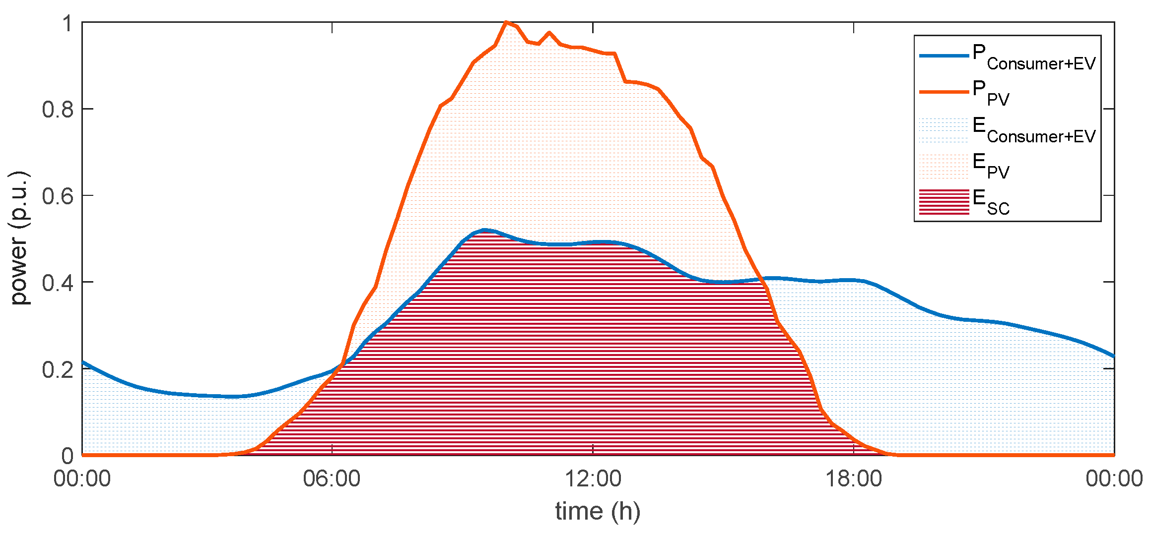
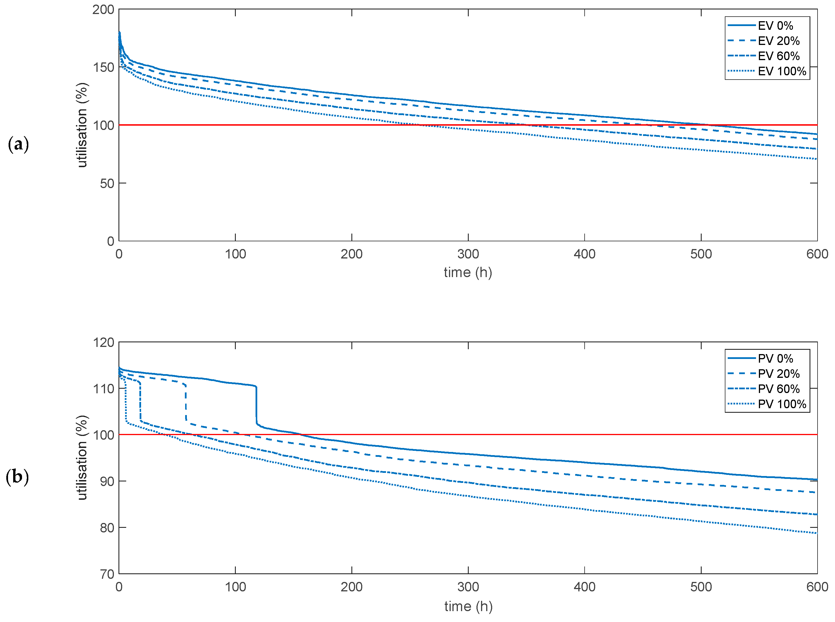
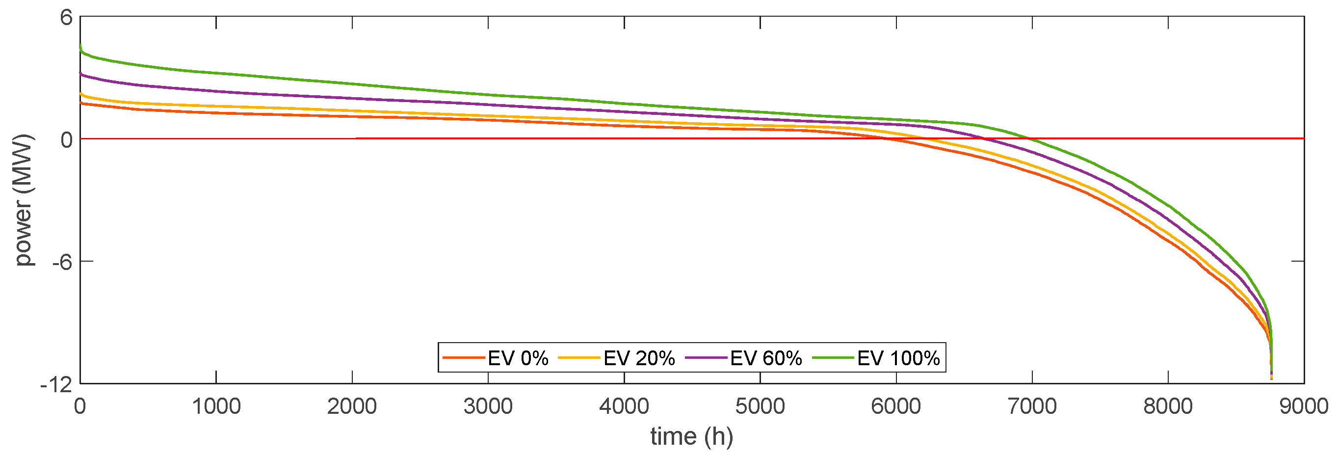
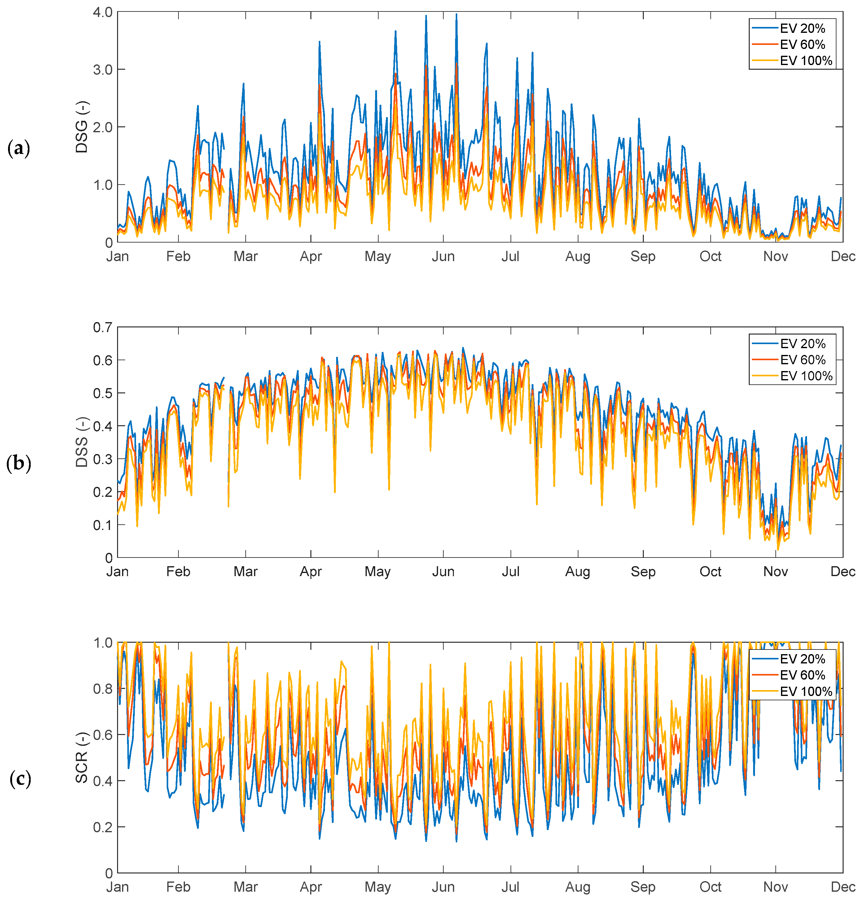
4.3. Energy Analyses

In the energy analysis depicted here, we show the interaction of the energy flows between the cells and their significance for line overloads on the basis of the determined energy demand of e-mobility and the potential of PV production. Furthermore, we present the results on the energetic synergy effects between e-mobility and PV potential for different scenarios, which are based on the determination of the key performance indicators explained in Section 3.3. The key performance indicators are determined and analysed for each cell and the overall system regardless of grid parameters.

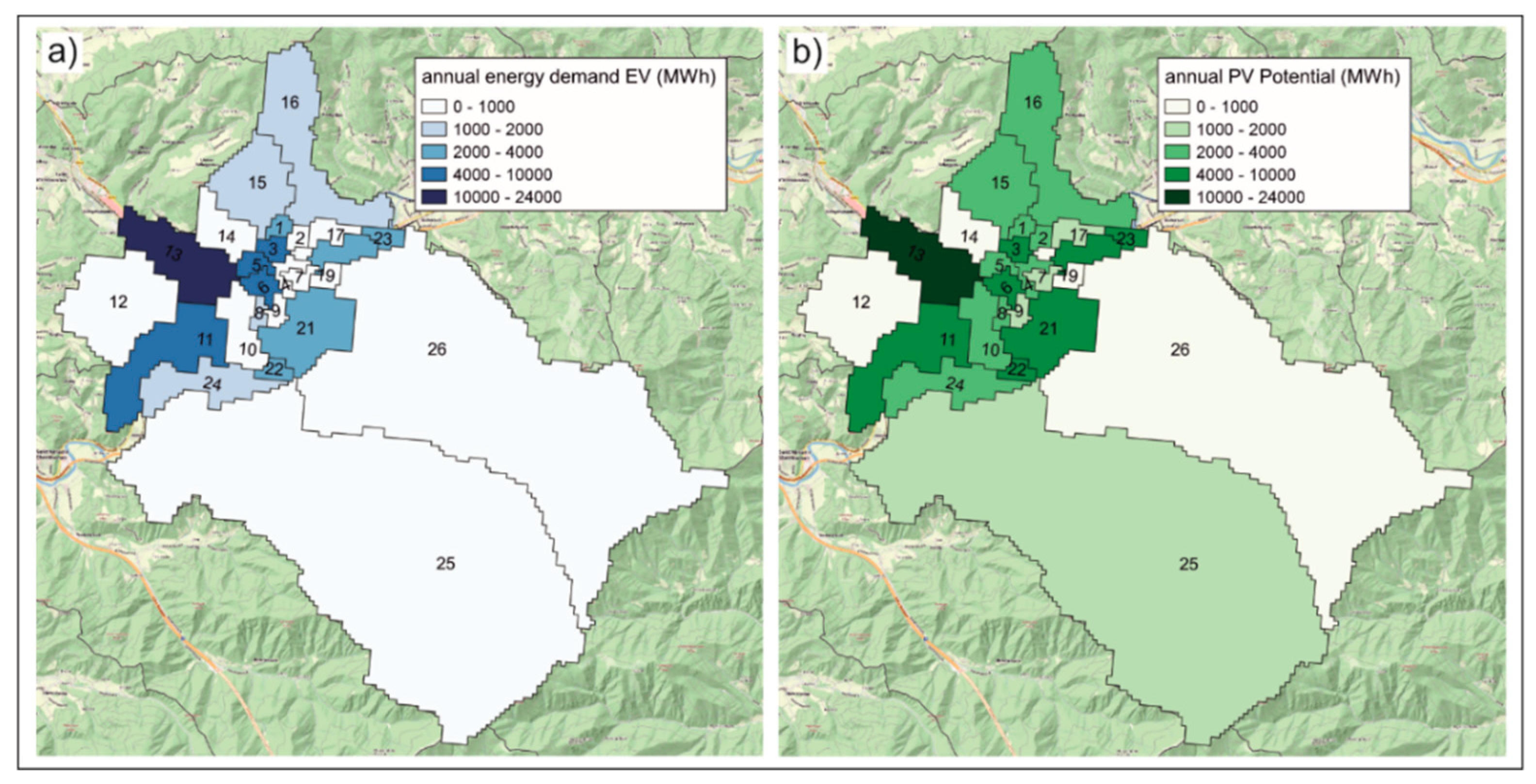
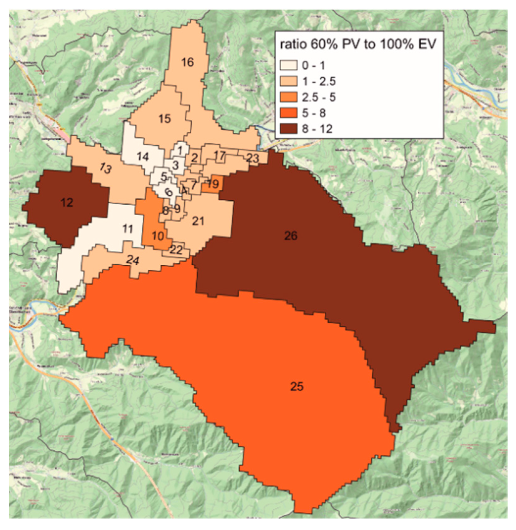
4.3.1. Interaction of Energy Surpluses between the Cells

The annual energy demand for each cell is determined on the basis of the synthetic charging profiles for e-mobility. Figure 18a illustrates the annual energy demand spatially resolved for a penetration of 100% EV. Depending on the cell, the annual energy demand is in the range of 20 MWh (cell 26) to 12,500 MWh (cell 13). Figure 18b shows the determined annual energy production of the PV potentials for a penetration of 100% spatially resolved. Depending on the cell, these vary between 290 MWh (cell 19) and 22,500 MWh (cell 13).

In addition to the highest PV potential and the highest demand for work-related e-mobility, cell 13 is a very industry intensive cell. Furthermore, two of the three lines connecting cell 13 with its neighbour cells are among the most stressed lines (line 1 and line 3). The overloads of the lines 1 and 3 are mainly caused by the PV potentials. Moreover, lines 1 and 3 belong to a closed ring system in which another most stressed line (line 2) is located. Figure 19 shows a schematic section of the cell-based grid model shown in Figure 10 and the relevant load flows for the closed ring structure. The directions of the load flows correspond to those at the time of the maximum utilisation of line 1 for a penetration of 60% PV and 100% EV, a charging power of 3.7 kW and charging strategy 1. For this time step, the directions of the load flows indicate that the unused PV potential of cell 12 covers the electricity demand of the cells 5, 6 and 14 (ratio PV to EV < 1, see Figure 20) and leads to a feed into the 30 kV level.

As already mentioned, the optimal ratio between e-mobility and PV potential is important to avoid overloads. For this purpose, Figure 20 shows the energetic ratio of the annual energy production of 60% of the PV potential to the annual energy demand for 100% e-mobility. The ratio varies between 0.42 (cell 1) and 11.45 (cell 26). While cell 13 has a ratio between e-mobility and PV potential of 1.07 for these penetrations, the neighbour cell (cell 12) with a ratio of 8.43 has a significant production surplus. This surplus is transported from cell 12 to cell 13 and from there via lines 1 and 3 to cells 5 and 10, where this surplus leads to overloads. To reduce overloads caused by the PV potential that cannot be avoided at a penetration of 100% EV, it is sometimes necessary to reduce the PV potential of these cells from a penetration of 60% to 40%.

An optimal energetic ratio between e-mobility and PV potential is, however, not sufficient to avoid overloads, since the annual energy demand of e-mobility does not allow conclusions to be drawn about the load curve and thus about the power ratio of the individual time step. This means that with an energetic optimum, there can be significant differences in the peak values between e-mobility and PV potential on the one hand, and a time shift between the two peaks on the other. Cell 13, for example, is characterised by shift operation and office workplaces. This characteristic results in a division of the energy demand into four load peaks. This means that the optimum balance between e-mobility and PV potential must be analysed and determined in terms of both energy and power.

The self-consumption of the cells, for example from households, also has an important influence on the cell balance and the load flows between the cells. For this reason, the self-consumption of the cells is taken into account in our further energy analyses.

4.3.2. Charging Strategy 1 – Uncontrolled Charging

The calculation of the residual load enables the determination of the maximum power surpluses and power demand. While the energetic ratio between 60% PV potential and 100% e-mobility is 1.07, Figure 21 shows that the power profile of the PV potential is significantly higher than the load demand (e-mobility and consumption) of cell 13. Due to this high difference, the PV production profile during the day can be seen from the residual load curve in Figure 21. The significant fluctuations in the negative residual load are due to the use of real irradiation and temperature data during the modelling of the PV potentials. The profiles therefore consider, for example, seasonal effects or shading by clouds. Especially at night, there is a positive residual load and thus an increased power demand. As shown in Figure 21a, depending on the weather, negative residual loads of up to 5 MW also occur in the worst-case week in winter. The residual load for the represented worst-case week in summer (identified in the grid study) indicates that June 5 is a cloudy and rainy day due to the predominantly positive residual load also during the day (see Figure 21b). With increasing penetration of EV and a fixed penetration of 60% PV, the power surplus of the PV potential decreases and the load demand at night increases, regardless of the season.

The sorted annual duration curve of the residual load of cell 13 in Figure 22 shows that in an observation period of one year, about 2/3 of the year show a positive residual load. In the last third, there is a rapid increase to a maximum power surplus of 11.8 MW at a penetration of 60% PV and no e-mobility. The influence of increasing e-mobility at a fixed penetration of 60% PV can be seen clearly from the annual duration curve. The curves are shifted in the direction of positive residual loads. In the case of a fixed penetration of EV and increasing penetration of PV, the annual duration curves behave in exactly the opposite way.

The key performance indicators DSG, DSS and SCR are determined for each day for the simulation period of one year and are presented in Figure 23 for cell 13 at a fixed penetration of PV and increasing penetration of EVs.

The DSG decreases with increasing penetration of EV at a fixed penetration of PV (Figure 23a) and vice versa. Due to the high-power profile of the PV potential compared to the synthetic charging load profile of cell 13, maximum DSG of up to four are possible (without EV). The DSS has its maximum in summer with up to 0.65. This means that up to 65% of the locally produced PV Potential can be consumed directly. The DSS behaves like the DSG, which means that the DSS decreases with increasing penetration of EV at a fixed penetration of PV (Figure 23b) and vice versa. The seasonal dependence is less significant for SCR compared to DSG and DSS. In contrast to the DSG and DSS, the SCR increases with increasing penetration of EV at a fixed penetration of PV (Figure 23c) and vice versa.

4.3.3. Charging Strategy 2 – Controlled Charging

To determine the influence of controlled charging on the key performance indicators, two scenarios are compared, which differ only in the charging strategy. The basis for the results presented below is based on scenarios, which assume a fixed penetration of 60% PV, an increasing penetration of EV and a charging power of 3.7 kW. For the analysis, we take the cells 4, 5, 13 and 18 into account. Figure 24 shows the maximum and minimum relative deviation of selected cells that occur within the comparison of DSG, DSS and SCR of the respective scenarios. The relative deviation varies between −0.16 and 0.31 and is calculated for the respective key performance indicators (KPI) as follows:

$$relative deviation=\frac{KP{I}_{charging strategy 2}-KP{I}_{charging strategy 1}}{KP{I}_{charging strategy 1}}$$

(5)

Since the focus of the presented case study is on the user group “charging at work” and these charging processes take place mainly during the day, the daily energy demand of e-mobility remains almost constant on weekdays. On weekends, the user group “trip home” is also selected, where, as already mentioned, charging takes place mainly in the evening or at night. To avoid load peaks of the e-mobility in the evening, in charging strategy 2 these charging processes are distributed over the night, this can lead to shifts in energy demand from one day to the other. Among the other effects, this shift leads to the relative deviations of the DSG as shown in Figure 24a. Since the DSS and SCR calculate the directly consumed part of the locally produced energy on the basis of the total energy demand or the total locally produced energy, the positive relative deviations shown in Figure 24b,c are based on the time shift of the charging processes into the peak of the PV potential. The negative relative deviations, which mean, that controlled charging has a negative effect compared to uncontrolled charging, can be caused by both methods, shifting of the charging processes into the peak of the PV and sequencing the charging processes overnight. For instance, through the distribution of charging processes overnight, the evening peak of e-mobility is reduced. Since in summer there is often sufficient PV production until the evening hours, this reduction of the evening peak can lead to a lower use of the PV potential and therefore to a decrease of DSS and SCR. As shown in Figure 24 for different cells, the benefit of controlled charging (charging strategy 2) depends on the one hand on the user behaviour of the sector-specific jobs within the cells and on the other hand from the balance between energy demand and the PV potential. This means that the more charging processes take place in the early morning hours and can be shifted into the peak of the PV potential, the higher the DSS and SCR (positive relative deviation) with sufficient PV potential. However, if the ratio of EV to PV is very high, as for example in winter, the shifting of the charging processes has a minor influence on the DSS and SCR. Therefore, in addition to considering the optimal ratio between e-mobility and PV potential, the actual benefits of controlled charging should also be evaluated. However, applying controlled charging leads to a minor positive effect.

5. Conclusions

This paper presents results from a case study for the city of Leoben (Austria), which investigates the synergy effects between e-mobility charged only at work and photovoltaic potentials. The basis for the determination of the grid-side synergy effects is a cell-based grid model. Taking into account the spatial cell division of the grid model, load and production profiles, synthetic charging load profiles for e-mobility and PV potential profiles are determined. For different scenarios (variation of the penetration of EV and PV, charging power, charging strategy), load flow calculations are performed for a simulation period of one year. The results of the load flow calculations are investigated regarding grid-side synergy effects. Additionally, four key performance indicators (residual load, DSG, DSS and SCR) are used to analyse energetic synergy effects between e-mobility and PV potentials.

By using the cellular approach to develop a grid model, there is always a compromise between accuracy, resolution and calculation time. By aggregating the original power grid into energy nodes, this grid model is not suitable for detailed planning, but provides an overview of the effects caused by increasing e-mobility and PV potential. The possibility of carrying out simulations on the grid model for one year means that annual trends, worst-case days and weeks as well as countermeasures can be derived and analysed. As a result, these findings can be used as a basis for detailed studies on the original power grid.

The analyses of the grid-side effects show that with increasing penetration of EV and PV as well as increasing charging power, the grid utilisation and thus the number of line overloads increases. Although line overloads cannot be avoided completely, the maximum line utilisation and the duration of the overloads can be reduced by the correct ratio between e-mobility and PV potential. By using controlled charging (charging strategy 2), the charging processes are shifted to the peak of the PV potential, therefore the power requirement of e-mobility can increase. On the one hand, this increase relieves the grid because it reduces the excess power of the PV potential and on the other hand, it leads to an increased grid load if there is not sufficient PV production available. The comparison of a worst-case week in winter with one in summer shows the need to consider seasonal effects during grid-side and energy analysis. For example, with fixed penetration of PV and increasing penetration of EV, production surpluses are reduced in summer, while increasing e-mobility in winter leads to an increase in line utilisation due to insufficient PV potential. However, if the PV potential is much higher than the demand for e-mobility, controlled charging has little impact on the reduction of line utilisation and thus on overloads caused by PV potentials. Furthermore, the four key performance indicators of the energy analysis demonstrate the importance of modelling PV potentials using real irradiation and temperature data. Besides the residual load, which indicates the fluctuating power surplus caused by the PV potential, DSG, DSS and SCR vary significantly between two consecutive days. The investigation of the residual loads of different scenarios shows that high negative residual loads, which lead to overloads mainly in summer, are reduced by an increasing penetration of EV while the penetration of PV remains the same. However, since the overloads cannot be avoided completely, further possibilities to reduce these high negative residual loads, like a reduction of the PV potential or the use of controlled charging need to be considered. A reduction of the PV potential as well as the increasing e-mobility lead to increasing positive residual loads, especially in winter on PV production weak days. The use of controlled charging can reduce both, negative and positive residual loads. While negative residual loads are reduced by shifting the charging processes into the peak of the PV potential, positive residual loads are reduced by sequencing the charging processes.

The analysis of grid and energy-side effects has shown the importance of balancing e-mobility and PV potential. The same penetration of EV and PV over all cells for the scenarios considered leads to large differences in the ratios between the energy demand of e-mobility and the PV potential of the individual cells. With penetrations of 60% PV and 100% EV, these ratios are in the range of 0.42 (cell 1) to 11.45 (cell 26) based on the annual energy production of the PV Potential and the annual energy demand of e-mobility. Due to this uneven distribution, for example, a penetration of 100% EV can lead to a line overload, whereas this penetration would be necessary to reduce a power surplus of the PV potential in another cell.

In summary, the key findings of the grid-side and energetic synergy effects between e-mobility charged only at work and PV potentials for the presented case study are as follows:

• To avoid line overloads, spatial planning is important in addition to the optimal energy and power ratio between e-mobility and PV potential.
• The optimal ratio between e-mobility and PV potential is limited by the seasonal component. This means, for example, while increasing e-mobility in summer counteracts negative effects of the PV potential, it leads to higher line utilisations in winter.
• Controlled charging for charging at work has only a minor positive effect on line overloads and key performance indicators.

Although this study shows first trends for the synergies between e-mobility charged only at work and PV potentials, it is also subject to some limitations. Besides the limitations already mentioned, the lack of the possibility of detailed planning and constant penetration across all cells, the data basis is a dominating factor. The real irradiation and temperature data [14] and database for the electric power grid including consumption and generation data are from 2014. In addition, the traffic analyses and statistical data [23,24,25] used refer to today’s mobility behaviour and thus mainly to vehicles with combustion engines. New technologies open up new possibilities, which influence mobility behaviour and therefore change it. To model the synthetic charging load profiles, the vehicles registered in Germany up to 2018 [27] (battery capacity, average energy consumption and charging efficiency) are used. Furthermore, the focus of the presented case study is on a grid-side and energetic consideration, this means that no ecological and economic factors are taken into account. In the area of controlled charging, the trends of line overloads identified in this case study and the associated necessary grid expansion should be analysed in combination with economic and ecological strategies for controlled charging. Furthermore, the use of storage systems at strategic grid points to avoid overloads should be investigated in further studies. Due to the limiting factor of a constant penetration across all cells, following studies should analyse and determine the optimal ratio between e-mobility and PV potentials at cell level to define the scenarios. Based on this optimum per cell, the impact on the power grid should be analysed to verify the hypothesis that overloads can be avoided. The possibility of increasing the determined optimal penetration rate of EV or PV by controlled charging or by the use of storages should also be investigated.

References

1. Vopava, J.; Kienberger, T. Impact of increasing electric mobility on a distribution grid at the medium voltage level. In Proceedings of the 2nd E-Mobility Power System Integration, Stockholm, Sweden, 15 October 2018. [Google Scholar]
2. Clement-Nyns, K.; Haesen, E.; Driesen, J. The Impact of Charging Plug-In Hybrid Electric Vehicles on a Residential Distribution Grid. IEEE Trans. Power Syst. 2010, 25, 371–380. [Google Scholar] [CrossRef] [Green Version]
3. Deb, S.; Tammi, K.; Kalita, K.; Mahanta, P. Impact of Electric Vehicle Charging Station Load on Distribution Network. Energies 2018, 11, 178. [Google Scholar] [CrossRef] [Green Version]
4. Leemput, N.; Geth, F.; van Roy, J.; Olivella-Rosell, P.; Driesen, J.; Sumper, A. MV and LV Residential Grid Impact of Combined Slow and Fast Charging of Electric Vehicles. Energies 2015, 8, 1760–1783. [Google Scholar] [CrossRef] [Green Version]
5. Osório, G.; Shafie-khah, M.; Coimbra, P.; Lotfi, M.; Catalão, J. Distribution System Operation with Electric Vehicle Charging Schedules and Renewable Energy Resources. Energies 2018, 11, 3117. [Google Scholar] [CrossRef] [Green Version]
6. Munkhammar, J.; Widén, J.; Rydén, J. On a probability distribution model combining household power consumption, electric vehicle home-charging and photovoltaic power production. Appl. Energy 2015, 142, 135–143. [Google Scholar] [CrossRef]
7. Chaouachi, A.; Bompard, E.; Fulli, G.; Masera, M.; De Gennaro, M.; Paffumi, E. Assessment framework for EV and PV synergies in emerging distribution systems. Renew. Sustain. Energy Rev. 2016, 55, 719–728. [Google Scholar] [CrossRef]
8. Su, S.; Hu, Y.; Yang, T.; Wang, S.; Liu, Z.; Wei, X.; Xia, M.; Ota, Y.; Yamashita, K. Research on an Electric Vehicle Owner-Friendly Charging Strategy Using Photovoltaic Generation at Office Sites in Major Chinese Cities. Energies 2018, 11, 421. [Google Scholar] [CrossRef] [Green Version]
9. Chandra Mouli, G.R.; Bauer, P.; Zeman, M. System design for a solar powered electric vehicle charging station for workplaces. Appl. Energy 2016, 168, 434–443. [Google Scholar] [CrossRef] [Green Version]
10. Gnann, T.; Klingler, A.L.; Kühnbach, M. The load shift potential of plug-in electric vehicles with different amounts of charging infrastructure. J. Power Sources 2018, 390, 20–29. [Google Scholar] [CrossRef]
11. Vopava, J.; Koczwara, C.; Traupmann, A.; Kienberger, T. Investigating the Impact of E-Mobility on the Electrical Power Grid Using a Simplified Grid Modelling Approach. Energies 2020, 13, 39. [Google Scholar] [CrossRef] [Green Version]
12. Babrowski, S.; Heinrichs, H.; Jochem, P.; Fichtner, W. Load shift potential of electric vehicles in Europe. J. Power Sources 2014, 255, 283–293. [Google Scholar] [CrossRef] [Green Version]
13. Su, W.; Wang, J.; Zhang, K.; Chow, M.Y. Framework for investigating the impact of PHEV charging on power distribution system and transportation network. In Proceedings of the IECON 2012, 38th annual conference on IEEE Industrial Electronics Society, Montreal, QC, Canada, 25–28 October 2012; pp. 4735–4740, ISBN 978-1-4673-2421-2. [Google Scholar]
14. ZAMG Zentralanstalt für Meteorologie und Geodynamik. Einstrahlungsmessdaten und Temperaturmesswerte des Jahres 2014 für Kapfenberg; ZAMG Zentralanstalt für Meteorologie und Geodynamik: Wien, Austria, 2014. [Google Scholar]
15. Amt der Steiermärkischen Landesregierung. Solardachkataster Steiermark. Available online: https://www.landesentwicklung.steiermark.at/cms/beitrag/11864478/142970647/ (accessed on 3 July 2020).
16. Zhang, T.Z.; Chen, T.D. Smart charging management for shared autonomous electric vehicle fleets: A Puget Sound case study. Transp. Res. Part D 2020, 78, 102184. [Google Scholar] [CrossRef]
17. Steinmüller, H.; Tichler, R.; Kienberger, T.; Gawlik, W.; Lehner, M.; Muggenhumer, G.; Kriechbaum, L.; Böckl, B.; Winter, A.; Biegger, P.; et al. Smart Exergy Leoben—Final Report. Exergetische Optimierung der Energieflüsse für eine smarte Industriestadt Leoben; Klima- und Energiefonds: Wien, Austria, 2017. [Google Scholar]
18. Kienberger, T.; Hammer, A.; Vopava, J.; Thormann, B.; Kriechbaum, L.; Sejkora, C.; Hermann, R.; Watschka, K.; Bergmann, U.; Frewein, M.; et al. Move2Grid—Final Report. Umsetzung regionaler Elektromobilitätsversorgung durch hybride Kopplung; Bundesministerium für Verkehr, Innovation und Technologie: Wien, Austria, 2019. [Google Scholar]
19. NEPLAN AG; NEPLAN: Küsnacht, Switzerland, 2015.
20. BDEW—Budesverband der Energie- und Wasserwirtschaft e.V. Standardlastprofile Strom. Available online: https://www.bdew.de/energie/standardlastprofile-strom/ (accessed on 3 April 2019).
21. E-CONTROL. Sonstige Marktregeln. Kapitel 6: Zählwerte, Datenformate und Standardisierte Lastprofile. Available online: https://www.e-control.at/recht/marktregeln/sonstige-marktregeln-strom#p_p_id_56_INSTANCE_10318A20066_ (accessed on 3 April 2019).
22. QGIS Development Team. QGIS Geographisches Informationssystem. Available online: https://qgis.org/en/site/ (accessed on 3 July 2020).
23. Bosserhoff, D. Integration von Verkehrsplanung und Räumlicher Planung. Teil2: Abschätzung der Verkehrserzeugung Durch Vorhaben der Bauleitungsplanung; Hessisches Landesamt für Straßen- und Verkehrswesen: Wiesbaden, Germany, 2000. [Google Scholar]
24. Fraunhofer-Institut für System- und Innovationsforschung ISI. Codebook REM 2030 Driving Profiles Database; Fraunhofer-Institut für System- und Innovationsforschung ISI: Karlsruhe, Germany, 2015. [Google Scholar]
25. Infas—Institut für angewandte Sozialwissenschaft GmbH; TRICONSULT—Wirtschaftsanalytische Forschung Gesellschaft m.b.H; HERRY Consult GmbH; Sammer und Partner Zivilingenieur GmbH, ZIS+P Verkehrsplanung; Institut für Verkehrswesen der Universität für Bodenkultur. Österreich Unterwegs 2013/2014. Ergebnisbericht; Bundesministerium für Verkehr, Innovation und Technologie: Wien, Austria, 2016. [Google Scholar]
26. Infas-Institut für angewandte Sozialwissenschaften GmBH; Deutsches Zentrum für Luft und Raumfahrt e.V.; Institut für Verkehrsforschung; IVT Research GmbH. Mobilität in Deutschland—MiD. Ergebnisbericht; Bundesministerium für Verkehr und digitale Infrastruktur: Bonn, Germany, 2018. [Google Scholar]
27. Kraftfahrt-Bundesamt. Neuzulassungen—Deutschland. Available online: https://www.kba.de/DE/Statistik/Fahrzeuge/Neuzulassungen/neuzulassungen_node.html (accessed on 15 July 2019).
28. Allgemeiner Deutscher Automobil-Club e.V. ADAC Ecotest. Available online: https://www.adac.de/infotestrat/tests/eco-test (accessed on 1 July 2019).
29. Tober, W. Praxisbericht Elektromobilität und Verbrennungsmotor. Analyse elektrifizierter Pkw-Antriebskonzepte; Springer: Wiesbaden, Germany, 2016; ISBN 9783658136017. [Google Scholar]
30. World Meteorological Organization. Mean Daily Temperature Provided for Each Month by “World Weather Information Service”. Available online: https://www.wwis.dwd.de/de/home.html (accessed on 3 July 2020).
31. Kapfenberger-Pock, A. Grazer Solardachkataster. Solarthermie bzw. Photovoltaik; Stadtvermessungsamt: Graz, Austria, 2013. [Google Scholar]
32. Perez, R.; Seals, R.; Ineichen, P.; Stewart, R.; Menicucci, D. A new simplified version of the perez diffuse irradiance model for tilted surfaces. Sol. Energy 1987, 39, 221–231. [Google Scholar] [CrossRef] [Green Version]
33. Perez, R.; Stewart, R.; Seals, R.; Guertin, T. The Development and Verification of the Perez Diffuse Radiation Model; Sandia National Labs: Livermore, CA, USA, 1988. [Google Scholar]
34. Perez, R.; Ineichen, P.; Seals, R.; Michalsky, J.; Stewart, R. Modeling daylight availability and irradiance components from direct and global irradiance. Sol. Energy 1990, 44, 271–289. [Google Scholar] [CrossRef] [Green Version]
35. Duffie, J.A.; Beckman, W.A. Solar Engineering of Thermal Processes, 3rd ed.; Wiley: Hoboken, NJ, USA, 2006; ISBN 9780471698678. [Google Scholar]
36. Pretschuh, P. Solares Energiepotential Kleiner und Mittlerer Städte; Montanuniversität Leoben: Leoben, Austria, 2016. [Google Scholar]
Figure 1. Original destination matrices according to Bosserhoff [23] and cumulative distribution function (a) trip home; (b) trip to work—shift operation. Reproduced from [11].
Energies 13 03795 g001
Figure 2. Visualization grid point, energy cell and energy node.
Energies 13 03795 g002
Figure 3. Example of suitable roof areas, including the classification “very good” and “good” based on data from the solar roof register [15].
Energies 13 03795 g003
Figure 4. Overview: development of a simplified cell-based model.
Energies 13 03795 g004
Figure 5. Overview: determination of synthetic charging load profiles of electric vehicles.
Energies 13 03795 g005
Figure 6. Determination of total distance travelled for each trip of the selected user groups.
Energies 13 03795 g006
Figure 7. Generic examples of charging processes, which can be shifted in or within the time span in green and those, which cannot in red.
Energies 13 03795 g007
Figure 8. Relevant areas for calculating the DSG, DSS and SCR.
Energies 13 03795 g008
Figure 9. Generic example of a load profiles of the user groups “trip to work” and “trip for shopping” as well as a PV production profile.
Energies 13 03795 g009
Figure 10. Simplified cell-based grid model for the city of Leoben.
Energies 13 03795 g010
Figure 11. Number of overloaded lines of the 5 kV voltage level for charging strategy 1.
Energies 13 03795 g011
Figure 12. Cell division of the city of Leoben and detailed view with geographical location of the identified overloaded lines - in red: most stressed lines.
Energies 13 03795 g012
Figure 13. Month of occurrence for the maximum line utilisation of all scenarios with charging strategy 1 during the simulation period of one year.
Energies 13 03795 g013
Figure 14. Annual duration curve of the utilisation for the period 0 to 600 h for 3.7 kW charging power and charging strategy 1 (a) line 1 and a fixed penetration of 60% PV (b) line 5 and a fixed penetration of 60% EV.
Energies 13 03795 g014
Figure 15. Comparison of the utilisation of the line 1 for a penetration of 40% EV and 60% PV with 3.7 kW charging power and charging strategy 1 and 2 for (a) 24 January (b) 2 June.
Energies 13 03795 g015
Figure 16. PV potential profile and synthetic charging load profiles for the e-mobility with 3.7 kW charging power, charging strategy 1 and 2 for cell 13 (a) 24 January (b) 2 June.
Energies 13 03795 g016
Figure 17. Sorted duration curve of the utilisation of line 1 at a fixed penetration of 60% PV and 3.7 kW charging power for the selected worst-case weeks (a) winter (b) summer.
Energies 13 03795 g017
Figure 18. (a) Annual energy demand e-mobility and (b) annual PV potential at cell level for the city of Leoben.
Energies 13 03795 g018
Figure 19. Schematic grid section - illustration of the direction of load flows for a penetration of 60% PV and 100% EV, 3.7 kW charging power and charging strategy 1 for the time of maximum utilisation of line 1.
Energies 13 03795 g019
Figure 20. Energetic ratio of the annual energy production of 60% PV potential to the annual energy demand of 100% EV.
Energies 13 03795 g020
Figure 21. Residual load of cell 13 for the selected worst-case weeks for a fixed penetration of 60% PV and a variation of the penetration of EV for 3.7 kW charging power and charging strategy 1 as well as for the reference scenario (without PV and EV) (a) winter (b) summer.
Energies 13 03795 g021
Figure 22. Sorted duration curve of the residual load of cell 13 for a fixed penetration of 60% PV and a variation of the penetration of EV for 3.7 kW charging power and charging strategy 1 and a simulation period of one year (8760 h).
Energies 13 03795 g022
Figure 23. Key performance indicator of cell 13 for the simulation period of one year and for a fixed penetration of 60% PV and a variation of the penetration of EV for 3.7 kW charging power and charging strategy 1 (a) DSG (b) DSS (c) SCR.
Energies 13 03795 g023
Figure 24. Maximum and minimum relative deviation of selected cells for a fixed penetration of 60% PV and a variation of the penetration of EV for 3.7 kW charging power (a) DSG (b) DSS (c) SCR.
Energies 13 03795 g024