Abstract
Recently, electric vehicles (EVs) have become an increasingly important topic in the field of sustainable transportation research, alongside distributed generation, reactive power compensation, charging optimization, and control. The process of loading on existing power system infrastructures with increasing demand requires appropriate impact indices to be analyzed. This paper studies the impact of integrating electric vehicle charging stations (EVCSs) into a residential distribution network. An actual case study is modeled to acquire nodal voltages and feeder currents. The model obtains the optimal integration of solar photovoltaic (PV) panels with charging stations while considering reactive power compensation. The impact of EV integration for the case study results in two peaks, which show a 6.4% and 17% increase. Varying the inverter to the PV ratio from 1.1 to 2 decreases system losses by 34% to 41%. The type of charging is dependent on the maximum penetration of EVCSs that the network can install without system upgrades. Increasing the number of EVCSs can cause an increase in power system losses, which is dependent on the network architecture. Installing PV reduces the load peak by 21%, and the installation of PV with consideration of reactive power control increases system efficiency and power delivery.
1. Introduction
Under the Paris Agreement signed in 2016, nine countries pledged to cut the world’s emissions by 2030. Transportation is the second-highest contribution to worldwide emissions, and it is expected to increase 60% by 2050 in the absence of mitigation measures [1]. To meet emission reduction goals, it is essential to expedite the adaptation of electric vehicles (EVs), which are currently being promoted to replace conventional vehicles, thus taking the EV market to a new level [2]. The success of this transition depends on the ability to provide adequate EV charging stations, which, in turn, must provide adequate power for the charging demands of EVs’ batteries. It is anticipated that the increasing rate of EVs will lead to a high electricity demand burden on the power grid.
1.1. Impact of EV Charging on Power Distribution Systems
The overall impact of EVs on the power distribution system was reviewed by [3]. This impact varies according to EV penetration, EV battery characteristics, charging demand, load characteristics, driving behavior, driving distance, demand response strategy, and electricity tariffs. The main identified problems were the increase in peak demand, power quality problems, power loss, transformer heating, and system overloading.
Connecting EV charging stations to the grid can negatively affect the power quality and efficiency of the network by introducing losses and voltage violations [4]. The optimal location and size of charging stations and renewable energy sources help to reduce this negative effect. The charging process has a direct effect on distribution system voltage levels; therefore, EV impact assessments are conducted for worst-case scenarios while modeling for EV electrical loads. Authors of [5,6] developed a model for EV load in MATLAB SIMULINK, which represented the behavior of the battery charge and discharge loading characteristics, and concluded that integrating EV fast-charging reduces the steady-state voltage stability limit of the power system.
The battery charge demand of an EV defines the impact on the power system. For instance, uncontrolled charging will cause the charging demand to require an upgrade to the power system, while controlled charging takes into account the distribution network’s constraints and does not require further upgrades to the network [7]. In other words, uncontrolled charging requires adding new equipment like transformers, cables, and protection devices to the existing distribution system in order to successfully host and deal with EV charging. Modeling the EV load can be done through a car trip destination based on the household and the person present, such as the Markov chain [8]. A probabilistic approach using the probability density function in modeling EV, grid loads, and PV outputs was reported by [9]. A stochastic modeling-implemented approach in the load flow based on the Monte Carlo method was discussed in [10]. The load demand of the EV fleet in [11] considers socio-economic, technical, and spatial factors. Deterministic EV load estimation based on actual measurements requires traffic data and surveys. The study in [12] suggested considering the degradation of EV batteries when sizing for renewable energy sources’ integration for EVCSs to avoid high-capacity sizing.
1.2. PV Implementation with EVCSs
Improving the distribution voltage levels affected by EV charging demand was suggested in [10] by combining PV systems with EV chargers, which proved effective in reducing system losses and in improving load profile and voltage levels. The modeled EV was modeled as a constant load, which was preliminary and did not reflect the actual load characteristics as proven in [6]. The authors of these papers did not incorporate the reactive power involved in EV chargers reported in [13].
To reduce the demand for EV charging of the electric grid, wind-powered EVCSs were suggested by [14]. A PV-based charging station with historical PV prediction was implemented in [15], which showed optimal performance. The author of [16] considered renewable energy technologies, including a diesel generator, concluded that a charging station with PV can benefit most when grid-connected.
Renewable energy sources, such as PV systems, have energy benefits regarding the grid, but may cause disturbances if not analyzed closely [17]. The increased penetration of distributed generation can lead to power system violations or problems such as voltage violations, line capacity or transformer overloading, and extreme line losses [18]. It is suggested in [15] that the most accurate hosting capacity limit for distributed generators (DGs) must be based on assessments of historical limits, performance limits, perception, and enhancement techniques. In other words, uncontrolled charging requires adding new equipment like transformers, cables, and protection devices so the existing distribution system can successfully host and deal with the EV charging.
1.3. Inverter Reactive Power
Modern inverters have the capability of providing reactive power support to improve voltage profiles and to minimize power losses, and therefore were investigated for the application of EV charging in [19]. According to the IEEE global community published standard for Interconnection and Interoperability of Distributed Energy Resources with Associated Electric Power Systems, namely IEEE 1574, there is no requirement for power factors [20]. On the other hand, in the international standard IEC 61727, the average lagging power factor of PV inverters is stated to be 0.9 when PV generation is 90% [21].
The charger also has the capability of allowing reactive power flow to the grid by utilizing the DC-link capacitor. Several authors have addressed this topic using the bi-directional EV battery charger enabled with the vehicle-to-grid (V2G) concept [22].
A control scheme in [23] implemented PV inverter reactive power compensation to improve network power quality, to reduce losses and overvoltage, and to increase renewable generation capacity. A method in [24] proposed an improved control response for grid inverter reactive power compensation, which controls the power flow between distributed generation and utility. An experimental study in [25] utilized the PV smart inverter as a Volt-Ampere reactive (VAr) controller to regulate the distribution voltage without the installation of additional devices.
1.4. Paper Contribution and Organization
Generally, the literature defines the impact of EV stations’ integration into the grid; however, most of the above-mentioned impact studies were performed at a unity power factor. Nowadays, grid-tie inverters can regulate their power factor by shifting their output voltage phase angle to supply or draw reactive power [19]. Another concern is that the increased demand for renewable energy sources (RESs) may have a negative effect on the distribution network [17], and enhancement techniques such as reactive power compensation will be considered alongside other factors while sizing for RES capacity [26]. According to a survey of the literature, most of the research concentrates predominantly on the impact of EV alone on power quality or with renewable energy sources, with less focus on the combined managed impact of EV with PV systems on the grid with reactive power control at non-unity operation.
This paper proposes analyzing the impact of EV integration on the distribution network by considering PV generation with reactive power compensation. This study suggests sizing the PV holding capacity based on enhancement techniques, such as system power loss minimizing. This capacity is based on considering the inverter size compared to the PV size, which is referred to as the inverter-to-PV ratio throughout this paper.
The summary of the proposed work is as follows: The maximum EV penetration for the distribution network is obtained for different scenarios. Subsequently, the optimal integration of solar PV with charging stations is obtained based on reactive power consideration and the inverter-to-PV ratio (power factor). The impact of the EV penetration level on the distribution system’s constraints is analyzed. The effect of reactive power generation on the grid on the impact study is considered. A forward/backward load flow model is used based on daily load profiles. Finally, modeling and simulation of a real-life residential area case study in Kuwait (Ahmadi) is carried out to obtain actual results.
The paper is structured as follows: In Section 2, the proposed approach for assessing the electric vehicle’s impact is explained; this section defines how to obtain EV charging demand, the PV capacity with its effect on the EV charging station, and the reactive power consideration from the PV inverter. Section 3 presents the models for the distribution network, the system load model, and the load flow problem. In Section 4, the case study explains the location of the test area, and the assumptions, considerations, and load profiles are defined. The results are presented and discussed in Section 5; this section considers the EVCS demand for an IEEE 33 bus, the EVCS demand of the Ahmadi residential area, the effect of PV inverter penetration on line losses with reactive power control, the effect of PV inverter power factors on PV optimum size, and a daily assessment of the power system for the Ahmadi distribution network with PV generation and EVCSs. The paper ends with a final summary of the findings and the conclusion in Section 6.
2. Proposed Approach for Assessing EV Impact
In this paper, different scenarios are considered to analyze the impact on the demands of EVCSs on the electric grid. The proposed approach considers EVCS to be the main load connected to the power system, rather than considering individual EVs as loads. Load flows are run to study the performance of distribution networks to assess certain performance and impact indices, such as nodal voltage variation and feeder overloading [26]. An approach for optimal PV integration is based on obtaining the optimal inverter size for power loss minimizing, considering the reactive power control capacity of the PV inverter. This method is based on the enhancement technique sizing of renewable sources in [15]. Finally, the effectiveness of this approach is assessed by analyzing the EVCS impact study combined with PV and reactive power control.
2.1. EV Charging Demand
The installation of EVCSs requires power system adequacy assessments. The concept of extra effective available energy determines the number of EV loads that can be connected to the system without infrastructure expansion [27]. The same concept was applied in this study to obtain the EVCSs’ maximum demand. The capacity of the chargers was obtained by load flow simulation, as explained in Figure 1a.
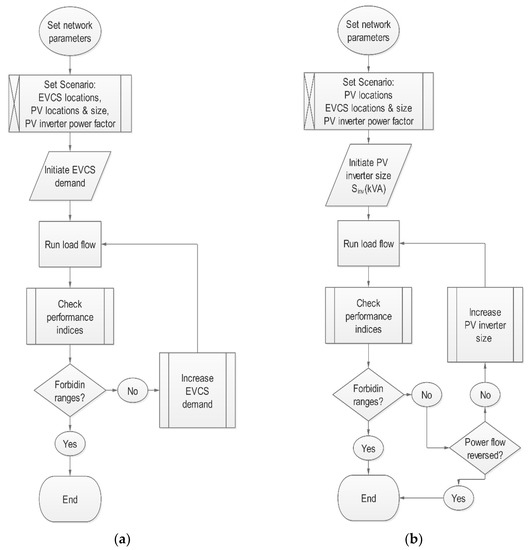
Figure 1.
Flow chart for (a) electric vehicle charging stations (EVCSs)’ maximum demand. (b) Maximum PV penetration. PV, photovoltaic; PF, power factor.
The load flow iteration obtains the maximum demand of EVCSs that can be added to the existing distribution system. The power system’s physical boundaries impose constraints on the voltage magnitudes () and phase angles ( and ) for all bus voltages in the power network.
The currents in the power lines must not exceed the rated value (1 p.u.), as in Equation (3).
To obtain the maximum demand for EVCSs, the power system is studied for worst-case scenarios when the loading is during peak hours. The actual maximum load demand for the case study was considered in the load flow.
2.2. PV Power with EVCSs
Overloading the power system with EVCSs impacts power system voltage profiles, line currents, and total losses, according to the system topology and physical characteristics. Through the paper; PT and QT refer to the power system’s total loading, while PT,i and QT,i refer to the power loading of a specific bus. Adding PV-distributed generation (PVDG) with EVCSs affects the overall loading of the power system. The main objectives of adding PVDG are:
- Line loss minimization
- Voltage profile improvement
- Increased power reliability
- Peak shaving
- Operation cost reduction
The total system power is therefore sum of the load (PL and QL), EV load (PEVCS and QEVCS), line losses (PLoss and QLoss), and PV inverter output power (−Pinv and ± Qinv). Therefore, the total active and reactive powers can be calculated as follows:
where, the negative sign at the inverter active power represents the direction of generated power (−) towards the grid. Also, the reactive power output of the inverter can either generate (−) or absorb (+) reactive power to or from the grid.
The maximum PV penetration is the capacity of the PV plant that can be added to the existing distribution network without the need for upgrading the infrastructure. The values of the maximum PV penetration are obtained by the optimum load flow, and the optimum solution is based on minimizing the line losses of the system without violating the physical constraints. The locations of the PV panels are predefined according to the available space.
2.3. Maximum PV Power Penetration
The PVDG connected to the distribution network acts as a negative load, as given in Equation (4). Increasing PV generation reduces line currents until the power flow is reversed. As the PV continues to increase, line currents start to increase, contributing to power system line losses, as calculated by (6):
The maximum active power the inverter can deliver from the PV plant at unity power factor is limited by the inverter’s size and efficiency. Otherwise, non-unity power factor operation allows the inverter the operation of reactive power injection or consumption.
This paper suggests obtaining the maximum PV penetration from the maximum apparent power of the inverter () at the worst-case (lowest) power factor operation using Equations (7)–(9).
where Qinv is the reactive power injected bythe EV charging inverter; Pinv is the active power injected by the inverter; is the angle between them; Sinv is the complex (active and reactive) power injected by the EV charging inverter; PF is the inverter power factor; ηinv is the inverter efficiency; PPV is the PV power; refers to the losses in the DC side (before inverter); and refers to the power losses in the PV.
DC system losses are taken into consideration when designing PV size, the calculation for which is as shown in Equation (9). Finally, the inverter-to-PV ratio is obtained according to this approach. The inverter size compared to the PV size is referred to as the inverter-to-PV ratio throughout this paper.
2.4. PV Inverter Reactive Power
The available reactive power at the inverters of EVCSs and PV can be utilized for reactive power compensation in order to improve power loss reduction and voltage profile. Line losses are a function of line current, as in Equation (6). Reducing line losses can be achieved by the PV inverter’s active and reactive power generation
Before adding the PV to the power system, the line current can be calculated as follow:
After adding PV to the distribution system, the line current can be calculated by Equation (11) as follow:
where V is the voltage between the two buses, and is the cable line in between. The available reactive power at the inverter is calculated by:
where Pinv can be the PV power at the PV inverter or the power consumed by the EV, which is considered an instantaneous value. Therefore, reactive power compensation application for voltage profile improvement can be realized when the EVCS is not receiving power [22].
3. System Modeling
3.1. The Distribution Network
Two distribution systems were studied. The first network is the IEEE 33 radial bus system, and the second network is an actual urban case study. Both systems are radial low-voltage (LV) systems, modeled in MATLAB code by defining busloads and line impedances. EVCSs were added to the connected loads at defined buses. PV solar power generation was considered for optimal integration at defined locations. The studies were repeated for multiple scenarios.
3.2. System Load Model
The different types of load models have a direct impact on distributed system planning [28]. The type of load models that are voltage-dependent, as defined in [29], are residential, commercial, and industrial loads. Voltage-dependent loads are calculated using Equations (13) and (14) and the values in Table 1.
where α is an active power exponent, β is the reactive power exponent, V is the bus voltage in per unit (p.u.), Po is the active power at rated voltage, and Qo is the reactive power at rated voltage.

Table 1.
Exponent values for residential loads.
3.3. The Load Flow Problem
The basic tool for electrical system analysis is the load flow, which was used to determine the performance of the system. The load flow involves finding the node voltages, line currents, and system losses that are necessary for optimizing network planning, the process of which involves repeating the load flow for multiple iterations. In the application of optimization, the efficiency of the load flow technique was considered.
The classification and comparison of load flow techniques were addressed by [30]. The popular backward-forward sweep (BFS) approach was used to determine the performance indices in the proposed study [31].
A distribution line illustrated in Figure 2 shows the effective active power Pi and reactive power Qi flowing in branch j through line resistance rj and reactance xj from node i to node i + 1.
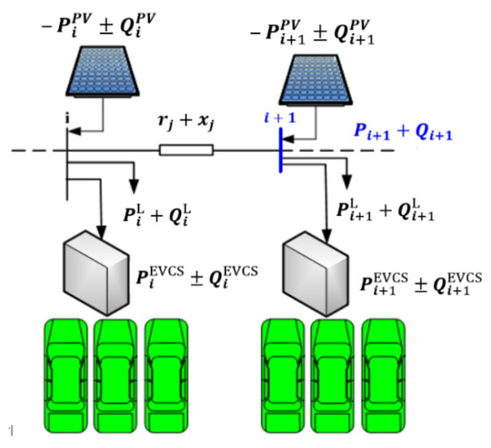
Figure 2.
Series impedance line and bus model.
The active and reactive powers can be calculated by Equations (15) and (16):
where PT,i+1 and QT,i+1 are the total active and reactive power at node i + 1, as formulated in Equations (17) and (18) without including both the EVCS and PV.
Considering both EVCS and PV implementation in the system, the total power equations are modified into Equations (19) and (20).
The magnitudes and phase angles of the voltages at each bus are calculated using Equations (21) and (22).
The total load Si on the main bus i is calculated using the bus voltage Vi and the outgoing feeder currents Ii by:
4. Case Study
4.1. The Test Area Description
To study the proposed assessment approach, a distribution network in an urban area located in Ahmadi, Kuwait, was considered. This section describes this base case study for the power system analysis. Kuwait has an area of 17,818 km2 with borders of about 195 km located along the Arabian Gulf (Figure 3).

Figure 3.
Illustration of Kuwait and Ahmadi city.
Ahmadi city is located 42 km south of Kuwait City and covers an area of 60 km2. This is a residential area for Kuwait Oil Company employees. The company provides housing, along with facilities and vehicles, and the residents of this area have a higher than average income. Therefore, the possibility of their owning EVs in the future may be higher than others in the country, which may be provided by the company or purchased using their own income. Therefore, analyzing the impact of EVs on this area is essential to promoting the first transition to EVs in Kuwait in the near future.
4.2. Assumptions and Considerations
The Ahmadi low-voltage (LV) residential network delivers power to domestic customers and operates on a medium-voltage to low-voltage (MV/LV) transformer, which supplies 40 houses with five outgoing pillars or feeders (Figure 4). The main transformer of the substation is loaded at 80% of its rated capacity.
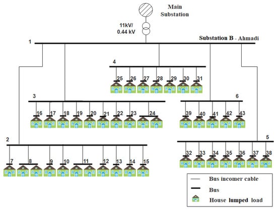
Figure 4.
Ahmadi residential network-typical.
All networks are assumed to be three-phase with balanced loads. Residential customers were modeled individually as lumped loads according to the main feeder maximum demand with an average power factor of 0.85.
Both the loading and the characteristic data of the network’s buses and lines were considered in this study. The cables feeding the customers were modeled according to their characteristics, sizes, and lengths. As shown in Table 2, the maximum current demand was measured during peak hours in Kuwait at 14:00 on 6 June.
Table 2.
Max current demand (6 June 2018 at 14:00).
The total number of EVCSs was chosen according to the required placement locations in the distribution network (see Figure 4 and Table 3).
Table 3.
Scenarios for the EV and PV locations for each case study.
It was assumed that only one EVCS is placed at each defined location/bus. The maximum capacity for the EVCS to be added to the network without violating the grid constraints was first obtained for every case study. Then, the optimal location of the PV was obtained for every EVCS location scenario. This was repeated for different values of the power factor. The reactive power at the inverter was taken into consideration for these scenarios by varying the PV inverter power factor (PF = 1, 0.9, and 0.8).
For the IEEE 33 bus system, the PV location was assumed to be at the EV charger bus. The impact assessment of EV charging on the Ahmadi residential area as performed when the chargers were at the residential buses as a case study. Another case was considered when charging was centralized at upper buses. The cases for the PVDG locations are defined in Table 4
Table 4.
Cases for PV locations.
4.3. PV and Load Profiles
After considering the impact of EVCSs on the grid during maximum demand (peak hours), a daily assessment of the power system was performed over a period of 24 h. during a summer peak day. The power flow was run with daily EVs, loads, and PV profiles to obtain the total power system load profile (see Table 5). The load profile was constructed from IEEE Reliability Test System (RTS) system [32]; see Table 5.
Table 5.
Daily variation % of peak load [32], EVCS hourly peak load in % daily peak load [27], and PV hourly generation for a 5 kWp plant in Kuwait on 11 June PVSYST© [33].
The hourly variation of the peak demand is provided as a percentage for every hour. The EVCS profile is based on the hourly peak loads as a percentage of daily peak loads. The individual house peak demand on the residential Ahmadi network is considered to be 22 kW. This is based on the data obtained from the site survey from the Kuwait Oil Company (KOC) housing team [34]. A rooftop PV power generation of 5 kW is obtained from the PVSYST© results in Table 5 and confirmed by capacity factors from the real-life PV rooftop projects installed in Kuwait [35]. The estimated PV generation is based on satellite data obtained for site location coordinates N 28°49′29.12″ (Latitude: 28.97), E 47°45′36.81″ (Longitude: 47.62).The actual meteorological data of the location is taken from satellite measures provided by SolarGIS [36]. The software used PVSyst© considers the location’s real temperatures and insulation on an hourly bases [33]. The electrical components are based on a typical PV rooftop system installed on the rooftop of a house in Kuwait City obtained from the contractor. According to the collected weather data, the peak irradiance in Kuwait occurred on 11 June. The hourly daily max demand load profile was constructed by PVSYST©; the selected PV panel type was Solar Frontier SF 155-S [37], and the inverter was PVI-6000-OUTD [38].
5. Results and Discussion
This section discusses the impact of EVCS penetration with PVDG and reactive power compensation on power system performance indices. The base case scenario is when there is no EVCS connected to the network system.
5.1. EVCSs’ Demand for IEEE 33 Bus
The IEEE 33 bus distribution system was used to investigate the model under study. The power system load flow results, represented as node voltages, line currents, and losses, were obtained for the different demands of the EVCS connected to the system. The results were assessed by the performance indices shown in Table 6. For all cases, the integration of the EVCS into the network system was limited by the capacity of the incoming feeder of the main bus 1, as shown in Figure 5.
Table 6.
Maximum EVCS penetration-demand obtained by load flow.
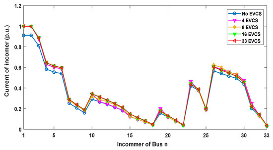
Figure 5.
Current in the incomer buses of 33 bus systems.
The limitation factor is defined by the incomer capacity, which should not exceed 1 p.u. Another limiting parameter is the voltage profile, which was taken into consideration while obtaining the EVCSs’ demand. The voltage profile at each bus was checked for all the scenarios, and also plotted in Figure 6.
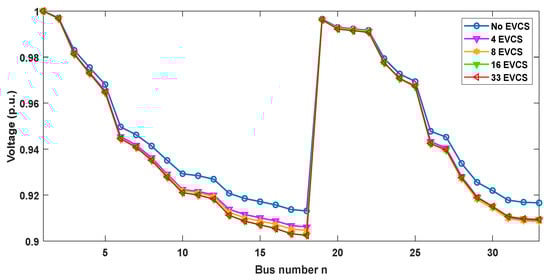
Figure 6.
Voltage profile for 33 bus distribution systems.
For the base case, the minimum voltage of 0.913 p.u. occurs at bus 18. This result was benchmarked and validated with the same bus voltage values published in [39,40]. The worst-case scenario was obtained for the maximum overloading of EVCSs, for which a voltage drop violation occurred.
For the IEEE 33 bus system with 33 integrated EVCSs, the voltage drop is approximately 1% compared only to the base case. In all cases, there is no voltage violation while integrating the maximum EV charger demand.
Figure 7 compares the line losses in the incoming lines (incomers) to the buses for all studied cases. It is observed that the incomers with most line losses are those for buses 2–6. It is also observed that the fewer the line losses, the greater the EVCSs’ installed capacity.
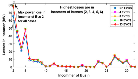
Figure 7.
Losses in the incoming lines of the buses in 33 bus systems.
The charging station’s maximum penetration for this IEEE 33 bus was obtained for the cases without PV. According to the results in Table 6, the capacity of the charging station is related to the number of total EVCSs distributed in the network.
For the case of four EVCSs in the network, the max capacity is 119 kW per charger station. This results in a higher total charging capacity of 476 kW in the overall system and lower losses of approximately 238 kW. Installing 33 EVCSs limits each charger to 14 kW. This case shows higher losses (244 kW) than the previous. The limitation factor in all cases is the incomer line capacity. For the IEEE 33-bus system, installing fewer EVCSs is more efficient than having higher numbers in the distribution network.
5.2. EVCSs’ Demand for the Ahmadi Residential Network
The maximum penetration of EVCSs at the Ahmadi Residential Network was obtained through load flow simulation, and the results are listed in Table 7. According to Figure 8, the maximum demand is limited by the maximum capacity of the incoming feeder to main bus 1.
Table 7.
Maximum EVCS penetration—demand obtained by load flow.
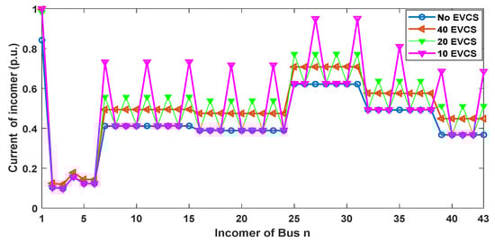
Figure 8.
Current in incomer buses of the Ahmadi distribution system.
Besides, the line currents are not uniformly drawn from the main bus because not all customers have charging stations installed at their bus/house. The load profile is less affected by these variations with the increase of customers with EV chargers integrated into the system.
Figure 9 shows the voltage profile at each bus. For the base case, the minimum voltage is found at buses 25 and 31 with a value of 0.95 p.u., which is within the acceptable limits. Notably, the maximum voltage drop for all cases under study is less than 1%.
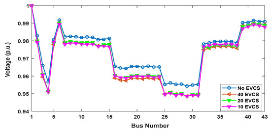
Figure 9.
Voltage profile for the Ahmadi distribution system.
In the case when all houses are equipped with EV chargers, which is equivalent to 100% EVCS integration, if the demand per charger is 4 kW, then the total charging demand is 160 kW. The analysis of this case scenario also shows less power loss in the network system. Figure 10 shows that the feeders of main buses 2–6 have the highest losses; these are the feeders of the main buses that feed multiple houses in parallel. Furthermore, the sizes of these feeders are 240 mm2 and run for approximately 300–700 m. The maximum ampacity (amperage) of the incomer of each feeder pillar at these buses is 400 A. The incomers to the rest of the buses are the residential buses, 185 mm2 in size, and run for approximately 30–200 m. For all cases, the currents in these lines reach maximum cable capacity because of the high charger loading current, in addition to the losses in the feeder line.
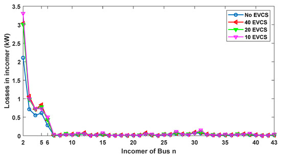
Figure 10.
Losses in incomers of the buses in the Ahmadi distribution system.
The limitation of this design is that fast charging cannot be implemented under the circumstances of only a 4 kW charging capacity. For the case with 10 EVCSs connected to the system (25% EVCS penetration), the capacity per charger is 15 kW, and the total charring demand is 150 kW. This case introduces higher line losses compared with the previous. As the number of EVCSs is reduced in this network, the individual charger capacity becomes larger. Consequently, the overall charging demand is decreased because of the increased line losses. Indeed, the line losses are directly affected by the EVCSs’ loading demand, location, number, and power line characteristics.
The plot in Figure 11 shows the overall active and reactive powers on the main bus (Bus 1) for different sizes of connected PV and EVCs. For the case of 100% EVCSs (40 EVCS) without integrating any PV power, the bus active power is 1354 kW and reactive power is 691 kVAr (blue), which is the transformer’s capacity 1.5 kVA.
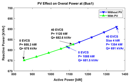
Figure 11.
System load at main bus (Bus 1) at 100% EVCS penetration (PV = 20 kW).
Notice that adding 20 kW PV power to the system reduces the total active load kW by 17.3% and kVA load by 14.5% (green). The following section studies the effect of PV penetration and inverter reactive power on power system line losses.
5.3. Effect of PV Inverter Penetration on Line Losses with Reactive Power Control
This paper proposes PV generation application with EV charging stations to minimize power system losses. The effect of PV penetration levels on power system losses was obtained through multiple iterations of the load flow simulation, with the objective to minimize power losses in the feeder lines. The results are presented in Figure 12, which are the losses obtained by the load flow for the Ahmadi network cases. The locations of the PV are mentioned in detail in Table 4.
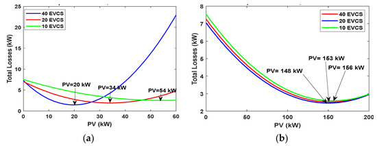
Figure 12.
Optimum PV size at minimum line loss for PV locations K1 and K2 for unity power factor: (a) Optimum PV at K1 locations; (b) optimum PV at K2 locations.
Line losses start decreasing with the increasing size of PV generation, and then start increasing at the point when PV generation exceeds the power at the bus and line losses. This is the point when the current is reversed. Therefore, the point of minimum power loss is the suggested optimal point of operation.
The maximum PV penetration for every case was obtained by the proposed load flow technique. The results are shown in Table 8 and Table 9. For the unity power factor, the PV rating was considered the inverter’s apparent power for the case study. For the IEEE 33 bus system, the PV locations were considered connected directly to the EVCS. PV generation introduces current to the network load, which in turn reduces losses in the lines by around 60–70% (see Table 8). This is the case when the PV inverter is operating at a unity power factor. As the PF decreases, the inverter compensates for the system’s reactive power. Setting the inverter power factor to 0.9 or 0.8 reduces line losses by approximately 90%. The maximum PV inverter penetrations for the Ahmadi distribution network are shown in Table 9. The results in Table 9 refer to the cases when EVCSs are connected at different capacities, and are as follows:
Table 8.
Effect of PV penetration on losses for the IEEE 33 bus system.
Table 9.
Effect of PV penetration on losses for the Ahmadi residential network.
Case 1: For 40 EVCSs in the system, the maximum PV inverter capacity obtained is 20 kW at the EVCS location and 153 kW if located at the main buses (2–6) for the unity power factor. The inverter size is increased when the power factor is reduced in order to obtain the optimum active and reactive power the system requires to minimize line losses. Therefore, at 0.9 power factor operation, the PV inverter size is 22 kW at the EVCS buses and 169 kW at the main buses. At 0.8 power factor operation, the change in the maximum size of the inverter is not significant.
Case 2: For 20 EVCSs in the system, the maximum PV inverter size obtained is 34 kW at the EVCS location (higher than Case 1) and 148 kW if located at the main buses (lower than Case 1) for the unity power factor. At 0.9 power factor operation, the PV inverter size is 38 kW at the EVCS buses and 166 kW at the main buses. At 0.8 power factor operation, the change in the maximum size is reduced. The reactive power generated by the inverter exceeds the load reactive power consumed by the power system load when the inverter operates at a power factor of 0.8.
Case 3: The maximum inverter size increases compared to Cases 1 and 2. The increase is more for the cases when the PV is installed directly at the main buses.
It is observed that, for the three cases, the maximum PV penetration is higher when the PV is installed at the EVCS buses when fewer EV chargers with higher capacity are connected to the system. For the Ahmadi distribution system, the line loss reduction for unity, 0.9, and 0.8 power factors is in the range of 60–80%, 80–90%, and 70–90%, respectively. Varying the inverter’s power factor results in a noticeable decrease in the line losses of both networks under study. In the load flow simulation, the value of apparent power was increased after each iteration, and the real and reactive power was calculated and added to the network. Thus, the numerical results can be used to develop a performance indicator that can be utilized for optimizing the inverter-to-PV ratio in the distribution network, along with EVCS planning.
5.4. Effect of PV Inverter Power Factor on PV Optimum Size
As the inverter power factor is reduced from unity, the optimum PV size kVA is affected. According to the results presented in Figure 13 and Figure 14, it is observed that the maximum PV penetration into the power system varies with the inverter power factor. For non-unity power factor operation, the optimum size of PV is chosen according to the optimum inverter-to-PV ratio for each power factor. This section did not consider the available area when calculating the maximum PV penetration. The inverter-to-PV ratios considered were 1 for PF = 1, 1.11 for PF = 0.9, and 1.25 for PF = 0.8. As the power factor decreases, the power system’s losses are lessened by reducing the reactive power load until the point where power losses start to increase, as for the case when PF = 0.8. The optimum inverter-to-PV ratio is 1.1 for this system. Changing the power factor setting of the inverter allows an increase in PV installation. Varying the inverter-to-PV ratio can affect the maximum connection that the system can allow. Therefore, the PV connection is more effective for systems with high line losses, as is the case when the PV is installed at the main buses (case in Figure 14).
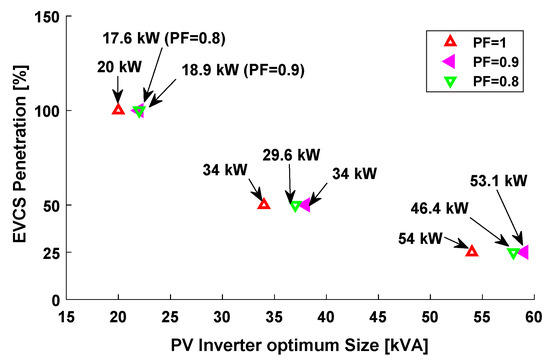
Figure 13.
Effect of PV inverter PF on PV optimum size—PV at EVCSs.
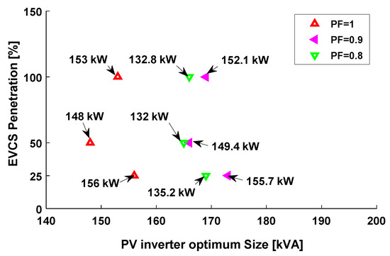
Figure 14.
Effect of PV inverter PF on PV optimum size—PV at main buses.
According to the Ahmadi distribution, the rooftop area of the residence can allow an installation of no more than 5 kW per house, which refers to the case study in the next section.
5.5. Daily Assessment of the Power System for the Ahmadi Distribution Network with EVCSs and PV
The daily load flow was obtained according to EVCSs’ demand, PV power generation, and PV inverter reactive power. The case under study was conducted with the following (obtained from previous results and assumptions):
Figure 15 shows the load profile for the Ahmadi distribution network, which is the overall active power drawn by the network at bus 1.
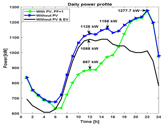
Figure 15.
Daily load profile at bus 1.
Case 1: The base case with zero EVCSs connected. The load profile shows an increasing peak around noon. The daily load profile is generated by the network’s maximum demand [32]. This case was studied according to the available data and the future development of the actual daily load demand required. The peak demand is approximately 1 MW and occurs between 11:00 and 15:00.
Case 2: This case studies the network at 100% EVCS penetration with no PV power. The EVCSs’ demand is reflected in the overall power profile. The increase in the load occurs at night between 16:00 and 07:00, which refers to the time during the weekdays where people return to their homes after work.
The noon peak increases by approximately 3.4%, and the new peak at 15:00 is 1.15 MW, which increases by 6.4%, with a higher peak at 22:00 of 1.27 MW (an increase of 17.4%). The load starts to reduce exponentially, which reflects the final behavior of the charging process of the electric vehicles’ batteries. Adding an EVCS to the load demand affects daily power losses by an increase of 17% (see Table 10).
Table 10.
Inverter power factor effect on system line losses.
Similar effect of EV charging on the load profile is found in the literature. The report in [41] shows two types of load factors (LFs) that of the load profiles. The system peak (SP) load factor and the non-coincident peak (NCP). The SP load factor is the ratio of the average EV demand to the EV peak demand, obtained here as 1.08. The NCP is the ratio between the average EV demand to the EV NCP demand, obtained here as 0.198.
Case 3: PV generation is the minimum where every house has an installation of only 4−5 kW, which operates around 2–3 kW per house. The total maximum PV generation occurs at noon, with approximately 130 kW, and load demand is reduced from 1.12 to 0.88 MW (a reduction of 21.4%). The power losses reduce by approximately 41% with PV generation (at 12:00 pm), as shown in Figure 16. At night, the PV inverter is used for reactive power compensation. The line losses are reduced by 16.6% during the night peak load (at 10 pm), and the daily power losses are reduced by 20% (see Table 10). This case considers the inverter-to-PV ratio to be 1; the available reactive power at the PV does not reach the installed capacity. Therefore, there is always available reactive power at the inverter to compensate for the system losses.
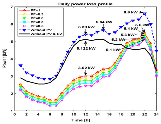
Figure 16.
Daily losses.
Case 4: The non-unity power factor of the PV inverter is considered. The effect of reactive power compensation is reflected in the line losses. PV generation is not affected by the power factor because the inverter-to-PV ratio is 1.11 for this case (PF = 0.9). The daily power losses are reduced by 2.5% compared with the case involving unity power factor operation.
Case 5: The inverter-to-PV ratio of this case is 1.25. The effect of having the inverter compensate at PF = 0.8 causes a 5.67% reduction in daily line losses compared to the system at a unity power factor.
Furthermore, other cases were considered for PF = 0.6 and 0.5, with an inverter-to-PV ratio of 1.5 and 2, respectively, with further daily loss reductions of 7.26% and 12.73%, respectively.
6. Conclusions
In this study, the impact of EV charging demand was analyzed for two case study power distribution networks with different characteristics. The power flow was validated by the standard IEEE 33 network. Different load flow scenarios were introduced to analyze the performance indices. Instead of varying the number of EVs, the number of EV charging stations was varied, and the maximum charging load capacity was obtained using the load flow analysis technique.
This paper suggests operating EVCS with PV power generation and reactive power compensation. The optimal PV size was considered by obtaining the optimum inverter-to-PV ratio for minimum power loss. The inverter optimum size was obtained at 0.9 power factor for the Ahmadi network without considering rooftop area limitations. The maximum PV size is not always the optimal solution when PVs are located at the same EVCS buses. Other cases show that reactive power increases the PV maximum penetration when the PV is located at the main feeder buses. The limitation factor refers to both cable ampacity and line losses at PV locations.
It was observed that PV integration with EV charging stations can decrease 21% of the load profile at noon in Kuwait. A high penetration of EV chargers among the houses in the Ahmadi case study causes a 17% increase in power demand at night. The increase does not exceed the network power system limitations for the worst-case scenario, which is the summer peak load. The capability for fast charging at residential areas is limited to the physical characteristics of the network. The maximum demand of an EVCS that can be provided for all customers is 4 kW, which limits the DC fast charging to be centralized at the network’s main buses only. Deciding whether or not to have central or distributed charging stations depends on both network characteristics and customer needs. Varying the Inverter to PV ratio from 1.1 to 2 can decrease the system losses by 34% to 41%, which shall be considered based on an economic assessment. Considering reactive power compensation with PVDG when integrating EVCS into the power system has triggered improvements in system efficiency and power delivery.
Author Contributions
Conceptualization, H.M.A.; formal analysis, H.M.A.; investigation, H.M.A. and R.M.K.; methodology, H.M.A.; project administration, A.G.; software, H.M.A. and A.T.; supervision, A.S. and A.G.; validation, R.M.K.; visualization, H.M.A. and A.T.; writing—original draft, H.M.A.; writing—review and editing, R.M.K and A.G. All authors have read and agreed to the published version of the manuscript.
Funding
This research received no external funding.
Acknowledgments
The technical support given by the Housing team of Kuwait Oil Company, which provided all of the necessary data required for modeling Ahmadi Residential Network in this study.
Conflicts of Interest
The authors declare that there is no conflict of interest.
Nomenclature
| Acronyms | Variables | ||
| DC | Direct Current | Pinv | Power injected by PV inverter (p.u) |
| DG | Distributed generator | PLoss | Total active power losses (p.u.) |
| EV | Electric vehicle | Po | Active power at rated voltage (p.u.) |
| EVCSs | Electric vehicle charging stations | PPV | PV active power (p.u.) |
| PV | Photovoltaic | QT | Total reactive power (p.u.) |
| PF | Power Factor | QL | Total load reactive power (p.u.) |
| PVDG | Photovoltaic distributed generation | QEVCS | Total EVCS reactive power (p.u.) |
| RES | Renewable Energy Sources | Qinv | Reactive power of PV inverter (p.u.) |
| Greek symbols | Qloss | Total reactive power losses (p.u.) | |
| δ | Angle of the bus voltage (degree) | Qo | Reactive power at rated voltage (p.u.) |
| ηinv | Inverter efficiency | Rline | Line resistance (ohm) |
| α | Active power exponent | Sinv | PV inverter apparent power (p.u.) |
| β | Reactive power exponent | Si | Apparent power at certain bus (p.u.) |
| Variables | Vi | Voltage of bus (p.u.) | |
| Iline | The line current (p.u.) | Vmin | Minimum limit of bus voltage (p.u.) |
| PT | Total active power of power system(p.u.) | Vmax | Maximum limit of bus voltage (p.u.) |
| PL | Total load active power (p.u.) | Xline | Line reactance (ohm) |
| PEVCS | Total EVCS active power (p.u.) | Zline | Line impedance (ohm) |
References
- Transport Outlook 2017.Enw. Available online: http://read.oecd-ilibrary.org/transport/itf-transport-outlook-2017_9789282108000-en#page1 (accessed on 23 May 2020).
- Wikström, M.; Eriksson, L.; Hansson, L. Introducing Plug-in Electric Vehicles in Public Authorities. Res. Transp. Bus. Manag. 2016, 18, 29–37. [Google Scholar] [CrossRef]
- Shareef, H.; Islam, M.M.; Mohamed, A. A review of the stage-of-the-art charging technologies, placement methodologies, and impacts of electric vehicles. Renew. Sustain. Energy Rev. 2016, 64, 403–420. [Google Scholar] [CrossRef]
- Moradi, M.H.; Abedini, M.; Hosseinian, S.M. Improving operation constraints of microgrid using PHEVs and renewable energy sources. Renew. Energy 2015, 83, 543–552. [Google Scholar] [CrossRef]
- Ma, G.; Jiang, L.; Chen, Y.; Dai, C.; Ju, R. Study on the impact of electric vehicle charging load on nodal voltage deviation. Arch. Electr. Eng. 2017, 66. [Google Scholar] [CrossRef]
- Dharmakeerthi, C.H.; Mithulananthan, N.; Saha, T.K. Impact of electric vehicle fast charging on power system voltage stability. Int. J. Electr. Power Energy Syst. 2014, 57, 241–249. [Google Scholar] [CrossRef]
- De Hoog, J.; Alpcan, T.; Brazil, M.; Thomas, D.A.; Mareels, I. Optimal charging of electric vehicles taking distribution network constraints into account. IEEE Trans. Power Syst. 2015, 30, 65–375. [Google Scholar] [CrossRef]
- Munkhammar, J.; Widén, J.; Rydén, J. On a probability distribution model combining household power consumption, electric vehicle home-charging and photovoltaic power production. Appl. Energy 2015, 142, 135–143. [Google Scholar] [CrossRef]
- Shariful Islam, M.; Mithulananthan, N.; Quoc Hung, D. Coordinated EV charging for correlated EV and grid loads and PV output using a novel, correlated, probabilistic model. Int. J. Electr. Power Energy Syst. 2019, 104, 335–348. [Google Scholar] [CrossRef]
- Tovilović, D.M.; Rajaković, N.L.J. The simultaneous impact of photovoltaic systems and plug-in electric vehicles on the daily load and voltage profiles and the harmonic voltage distortions in urban distribution systems. Renew. Energy 2015, 76, 454–464. [Google Scholar] [CrossRef]
- Hu, Q.; Li, H.; Bu, S. The prediction of electric vehicles load profiles considering stochastic charging and discharging behavior and their impact assessment on a real uk distribution network. Energy Procedia 2019, 158, 6458–6465. [Google Scholar] [CrossRef]
- Atia, R.; Yamada, N. More accurate sizing of renewable energy sources under high levels of electric vehicle integration. Renew. Energy 2015, 81, 918–925. [Google Scholar] [CrossRef]
- Haidar, A.M.A.; Muttaqi, K.M. Behavioral characterization of electric vehicle charging loads in a distribution power grid through modeling of battery chargers. IEEE Trans. Ind. Appl. 2016, 52, 483–492. [Google Scholar] [CrossRef]
- Lee, Y.; Hur, J. A simultaneous approach implementing wind-powered electric vehicle charging stations for charging demand dispersion. Renew. Energy 2019, 144, 172–179. [Google Scholar] [CrossRef]
- Ismaela, S.M.; Abdel-Aleemb, S.H.E.; Abdelazizc, A.Y.; Zobaad, A.F. State-of-the-art of hosting capacity in modern power systems with distributed generation. Renew. Energy 2019, 130, 1002–1020. [Google Scholar] [CrossRef]
- Hafez, O.; Bhattacharya, K. Optimal design of electric vehicle charging stations considering various energy resources. Renew. Energy 2017, 107, 576–589. [Google Scholar] [CrossRef]
- Kyritsis, A.; Voglitsis, D.; Papanikolaou, N.; Tselepis, S.; Christodoulou, C.; Gonos, I.; Kalogirou, S.A. Evolution of PV systems in Greece and review of applicable solutions for higher penetration levels. Renew. Energy 2017, 109, 487–499. [Google Scholar] [CrossRef]
- Gevers, D.N.; Aoki, A.R.; Impinnisi-Cleverson, P.R.; da Pinto, S.L.; da Damasceno, V.P.M.R. Evaluation of the impacts of renewables sources and battery systems in distribution feeders with different penetration levels. In Proceedings of the 2019 IEEE PES Innovative Smart Grid Technologies Conference-Latin America, Gramado, Brazil, 15–18 September 2019. [Google Scholar]
- Hung, D.Q.; Dong, Z.Y.; Trinh, H. Determining the size of PHEV charging stations powered by commercial grid-integrated pv systems considering reactive power support. Appl. Energy 2016, 183, 160–169. [Google Scholar] [CrossRef]
- IEEE 1547 Standard for Interconnecting Distributed Resources with Electric Power Systems. Available online: http://grouper.ieee.org/groups/scc21/1547/1547_index.html (accessed on 22 April 2020).
- IEC Standard. Photovoltaic (PV) Systems -Characteristics of the Utility Interface. Available online: https://www.iecee.org/dyn/www/f?p=106:49:0::::FSP_STD_ID:5736 (accessed on 22 April 2020).
- Yong, J.Y.; Ramachandaramurthy, V.K.; Tan, K.M.; Mithulananthan, N. Bi-directional electric vehicle fast charging station with novel reactive power compensation for voltage regulation. Int. J. Electr. Power Energy Syst. 2015, 64, 300–310. [Google Scholar] [CrossRef]
- Collins, L.; Ward, J.K. Real and reactive power control of distributed pv inverters for overvoltage prevention and increased renewable generation hosting capacity. Renew. Energy 2015, 81, 464–471. [Google Scholar] [CrossRef]
- Sampaio, L.P.; de Brito, M.A.G.; de Melo, A.G.; Canesin, C.A. Grid-tie three-phase inverter with active power injection and reactive power compensation. Renew. Energy 2016, 85, 854–864. [Google Scholar] [CrossRef]
- Howlader, A.M.; Sadoyama, S.; Roose, L.R.; Sepasi, S. Distributed voltage regulation using volt-var controls of a smart pv inverter in a smart grid: An experimental study. Renew. Energy 2018, 127, 145–157. [Google Scholar] [CrossRef]
- SIslam, M.S.; Mithulananthan, N. PV based EV charging at universities using supplied historical PV output ramp. Renew. Energy 2018, 118, 306–327. [Google Scholar] [CrossRef]
- Kamruzzaman, M.; Benidris, M. Effective accessible energy to accommodate load demand of electric vehicles. In Proceedings of the 2018 IEEE Industry Applications Society Annual Meeting (IAS), Portland, OR, USA, 23–27 September 2018; pp. 1–8. [Google Scholar] [CrossRef]
- Singh, D.; Misra, R.K. Load type impact on distribution system reconfiguration. Int. J. Electr. Power Energy Syst. 2012, 42, 583–592. [Google Scholar] [CrossRef]
- Price, W.W.; Casper, S.G.; Nwankpa, C.O.; Bradish, R.W.; Chiang, H.D.; Concordia, C.; Wu, G. Bibliography on load models for power flow and dynamic performance simulation. IEEE Trans. Power Syst. 1995, 10, 523–538. [Google Scholar] [CrossRef]
- Ghatak, U.; Mukherjee, V. An improved load flow technique based on load current injection for modern distribution system. Int. J. Electr. Power Energy Syst. 2017, 84, 168–181. [Google Scholar] [CrossRef]
- Augugliaro, A.; Dusonchet, L.; Favuzza, S.; Ippolito, M.G.; Sanseverino, E.R. A backward sweep method for power flow solution in distribution networks. Int. J. Electr. Power Energy Syst. 2010, 32, 271–280. [Google Scholar] [CrossRef]
- Laengen, Ø.S. Application of Monte Carlo Simulation to Power System Adequacy Assessment. Master’s Thesis, Norwegian University of Science and Technology, Trondheim, Norway, 2018. [Google Scholar]
- PVSyst. Available online: https://www.pvsyst.com/ (accessed on 22 April 2020).
- Al-Sabti, A. Meeting with the housing team in Kuwait oil company (KOC). In Proceedings of the SPE Kuwait Oil & Gas Show and Conference, Mishref, Kuwait, 13–16 October 2019. [Google Scholar]
- Life Energy Projects. Available online: http://www.thelifeenergy.com/projects/ (accessed on 22 April 2020).
- SolarGIS. Available online: https://solargis.com/ (accessed on 22 April 2020).
- Solar Frontier SF155-S (155W) Solar Panel. Available online: http://www.solardesigntool.com/components/module-panel-solar/Solar-Frontier/2294/SF155-S/specification-data-sheet.html (accessed on 22 April 2020).
- PVI-5000/6000-TL-OUTD-Legacy Solar Inverters (ABB Solar inverters). Available online: https://new.abb.com/power-converters-inverters/solar-old/legacy/pvi-5000kw-6000kw (accessed on 22 April 2020).
- Rupa, J.A.M.; Ganesh, S. Power flow analysis for radial distribution system using backward/forward sweep method. Int. J. Electr. Comput. Electron. Commun. Eng. 2014, 8, 5. [Google Scholar]
- Ahmed, A.H.; Hasan, S. Optimal allocation of distributed generation units for converting conventional radial distribution system to loop using particle swarm optimization. Energy Procedia 2018, 153, 118–124. [Google Scholar] [CrossRef]
- Electric Vehicle Charging Station; Xcel Energy: Minneapolis, MN, USA, 2015.


© 2020 by the authors. Licensee MDPI, Basel, Switzerland. This article is an open access article distributed under the terms and conditions of the Creative Commons Attribution (CC BY) license (http://creativecommons.org/licenses/by/4.0/).