Exergetic Evaluation of an Ethylene Refrigeration Cycle

Abstract

The production of light olefins by selective steam cracking is an energy-intensive process, and ethylene and propylene refrigeration cycles are key parts of it. The objective of this study was to identify opportunities for energy savings in an ethylene refrigeration cycle through an exergetic analysis. Two main causes of lower operational efficiency were identified: (1) Lower polytropic efficiency of the refrigerant compressor and (2) operating with the compressor mini-flow valve open to ensure reliability. The evaluation showed that the amount of irreversibilities generated by the cycle in operation is 22% higher than that predicted by the original design, which represents a 14% lower exergy efficiency. There is a potential savings of 0.20 MW in the cycle’s energy consumption with the implementation of the following improvements: recover refrigerant compressor efficiency by performing maintenance on the equipment and optimize the flow distribution between the recycle valve, the level control valve, and the temperature control valve.

1. Introduction

Selective cracking of hydrocarbons with steam, also known as steam cracking (SC), is the main production route of ethylene and other light olefins, such as propylene and butadiene [1]. Refrigeration cycles are fundamental for the operation of ethylene production plants and represent 15% to 20% of the total investment and 10% to 20% of the energy cost of an SC unit [2].

Because SC is a process with high energy demand, the energy cost is a relevant competitiveness factor for petrochemical sites around the world. It is estimated that in Brazil, the industry energy costs 46% higher than the international average, which increases the operational challenge of national ethylene production plants [3]. Therefore, studies that aims the reduction of energy consumption of through operational optimizations or structural changes, contribute to increase the competitiveness of ethylene production players.

Energy systems models are important methods used to generate a range of insight and analysis on the energy demand. These models and analysis have to be adequate to deal with the industrial energy challenges [4]. Moreover, according to [5], a description of technologies and procedures is missing in most of the end-use models for industrial systems, including the lack of real operating data that addresses the challenges experienced by the several types of processes that require a high energy demand. This is a serious omission for energy analysts, once energy consumption is driven by the diffusion of various types of equipment and the performance, saturation, and utilization of those equipment has a profound effect on energy demand.

To fill this knowledge gap, some authors use a thermodynamic modeling approach to identify opportunities of energy efficiency improvement. In [6], the authors use thermodynamic evaluation through modeling and simulation that were developed using compressor manufacturer’s data and real restrictions of each system component. In annual energy terms, the authors observed performance differences of 8% comparing different refrigeration architectures for commercial refrigeration.

Exergy determines the maximum work that can be achieved from a process or system when comparing its temperature, pressure, and composition conditions with a reference state [7]. Conventional exergy analysis is a powerful approach to assess energy systems since it not only quantifies inefficiencies but also helps qualify it. Conventional exergetic analyzes are not always able to assess the part of exergy that will inevitably be destroyed in each process. Thus, some authors recommend applying an advanced exergetic analysis, to distinguish the portion of the exergy destruction that is inevitable [8].

Analyses based on the first and second laws of thermodynamics have been performed for a transcritical N₂O refrigeration cycle and provide the theoretical basis for optimizing cycle design and operational control [9,10]. In [11], the authors use the currently considered the most effective thermodynamic tool to implement an exhaustive investigation with the aid of the advanced exergy analysis to analyze the performance of a transcritical CO₂ booster supermarket refrigeration unit. The application of the exergy analysis has provided additional and useful information to conclude that 59% of its inefficiencies can be reduced.

Emphasis is given to studies related to the use of exergetic analysis to identify opportunities for improving the energy efficiency of industrial processes, mainly based on the identification of points with greater exergy destruction and on the analysis of potential operational and equipment improvements [12,13]. This approach is also applied to natural gas treatment and refrigeration processes [14], to define the best refrigerant fluid [15] or the optimal mixture of refrigerant fluids [16]. Regarding the type of this work process, there are several reference studies with application in refrigeration cycles of petrochemical plants [17,18,19,20,21,22].

This study aims to identify opportunities for reducing the energy consumption of an ethylene refrigeration cycle of an existing petrochemical plant, through an exergetic evaluation. With this analysis, it is possible to quantify the exergy losses in each equipment of the cycle and propose changes in the operational conditions to improve the cycle efficiency. Although there are some applications of exergetic analysis in ethylene refrigeration cycles available in the literature, most of them rely on the evaluation of one operational case. In this work, the comparison of the design case and the current operating condition is applied to find the most significant energy improvement opportunities.

2. Methodology

The methodology chapter is divided into four sections: a short presentation of the refrigeration systems applied in the olefins plants and the description of the ethylene refrigeration cycle that is the object of study; the simulations premises and the thermodynamic model used; the equations applied for the exergy analysis, and the methodological approach used for identifying the main energy gaps.

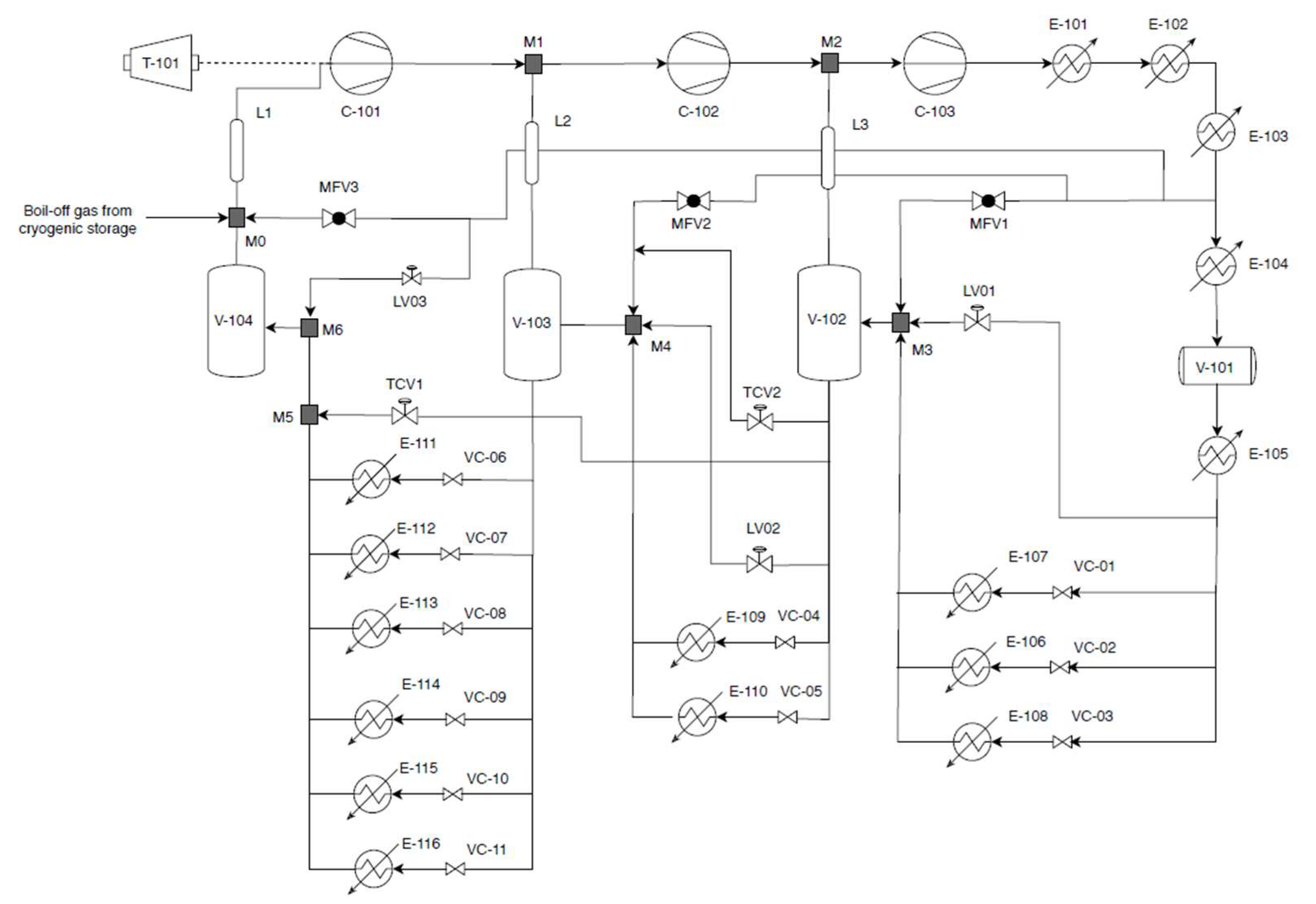
2.1. Refrigeration Systems Applied to Olefin Plants

Separation of the light hydrocarbons produced by SC is typically performed in high-pressure cryogenic systems, where refrigeration cycles are used to provide the cold streams needed to cool and condense the components present in the process.

Although the configuration and composition of the refrigerant fluids vary among plants, an olefin production plant typically has at least two refrigeration levels: the first up to −40 °C, using propylene as refrigerant, and the second up to −100 °C, using ethylene as refrigerant [23]. The propylene and ethylene refrigerant are multistage cascade cycles, which means that the discharge from the ethylene compressor is condensed with the lowest temperature level of the propylene cycle. The propylene cycle discharge pressure is defined so that condensation is possible using cooling water [2].

The propylene refrigerant compressor is typically a centrifugal compressor with one or two housings with three suction stages [24]. The main users of this cycle are the charge gas chillers, the ethylene fractionator condenser, the depropanizer column condensers, and the ethylene refrigerant cycle condensers. The ethylene refrigerant compressor is also typically a centrifugal compressor, with only one housing with three suction stages. The main users of this cycle are the low temperature charge gas chillers and the demethanizer condenser.

Despite having a single housing, such devices are commonly interpreted as compressors operating in series, each representing a refrigeration stage, connected to the same axis with a common drive. In this configuration, the vapor phase of each cycle stage is mixed with the discharge from the previous compressor. This representation is widely used in modeling this device, and the manufacturers also provide the performance curves of each stage as if they were independent machines.

Figure 1 presents the process scheme of the ethylene refrigeration cycle that is analyzed in this study. This cycle has three refrigeration stages, −55 °C, −75 °C, and −100 °C, driven by a multistage centrifugal compressor (C-101, C-102, and C-103) with a steam turbine (T-101).

Ethylene gas at high pressure is cooled with water in the E-101 exchanger, after which it is cooled, condensed, and subcooled by the E-102, E-103, E-104, and E-105 exchangers, which use propylene refrigerant at different temperature levels.

The liquid ethylene is then distributed to the users, where the pressure, and consequently the temperature, is reduced in the control valves (VC-01 to VC-11) located at the inlet of each heat exchanger. These exchangers are the evaporators of the cycle, also called users, which perform the cooling of various process streams.

Liquid ethylene not consumed by the users is sent in the liquid phase to the next stage by level control through valves LV01 and LV02. Although the presence of liquid is not expected in the last vessel, valve LV03 allows injecting ethylene gas from the compressor discharge to evaporate any liquid present due to occasional operational conditions where the cycle is unbalanced.

The main function of V-101 to V-104 drums is the separation of the liquid and vapor phase since the presence of liquid droplets in the compressor can cause significant damage to the interior of the machine. The gas phase of these vessels passes through lines L1, L2, and L3 before entering the suction end of one of the stages of the ethylene compressor. These lines were considered in the system model because they have a significant head loss by design.

The MFV1, MFV2, and MFV3 valves are the mini-flow valves of the compressor, which controls the anti-surge protection of this machine. Another relevant control is the temperature control of the first and second stages, which is performed by the TCV1 and TCV2 valves, that inject liquid ethylene from the third stage into the V-104 and V-103 vessels, respectively.

Operating with the mini-flow valve open increases the suction temperature of the compressor, since the ethylene used has a higher temperature than the fluid vaporized by the cycle users. Thus, the temperature control attenuates the increase and maintains the temperature of each stage. The adiabatic expansion that occurs in the temperature control valves (TCV1 and TCV2) generates a biphasic stream that is separated in the vessels, where the gaseous portion follow the compressor suction and the liquid phase is sent to the next stage by the level control. Vessel V-104 does not have drainage facilities and cannot send the liquid phase to any other vessel due to its low pressure. Thus, all the accumulated liquid must be vaporized by the LV03 valve, which uses ethylene after it exits exchanger E-103, which has a higher temperature.

Blocks M0 to M6 represent the mixing points of streams throughout the process. In actuality, mixing of the streams occurs in the pipes, but it is necessary to model these points this way because they act as direct contact heat exchangers since there may be a temperature difference between the streams that results in the generation of irreversibilities.

The boil-off gas stream from cryogenic storage shown in Figure 1 is the vapor phase generated in the cryogenic tanks of ethylene, which is sent to the suction of the compressor to be recycled.

2.2. Modeling the Ethylene Refrigeration Cycle

The refrigeration cycle was modeled using the commercial process simulator HYSYS^© (V10 from AspenTech, Bedford, MA, USA). The development of a process simulation is necessary to determine the thermodynamic properties of the process streams in the different evaluated cases.

For the ethylene refrigerant cycle simulation, the Peng-Robinson equation of state is used as the thermodynamic model. In addition to having well-known application in the representation of non-polar hydrocarbons over a wide pressure range, several studies recommended using the Peng-Robinson equation for the simulation of cycles of various refrigerant fluids, including the ethylene [15,18,19,25].

2.3. Exergy Analys

As mentioned, exergy is the maximum work obtained in a reversible process when a quantity of matter is moved from an initial condition to a state of equilibrium at a reference temperature and pressure. The equation representing the amount of specific exergy contained in a particular stream, commonly used in the exergy balance of several processes and devices that operate at steady state, disregarding the kinetic and potential energies, and when there are no chemical reactions or mixing effects, is represented by Equation (1):

$$\mathrm{ex}=\left(\mathrm{h}-{\mathrm{h}}_0\right)-{\mathrm{T}}_0\left(\mathrm{s}-{\mathrm{s}}_0\right)$$

(1)

Some equipment has more than one mathematical interpretation to calculate the irreversibilities and efficiency of the second law. The present study uses the equations contained in previous work [17,26,27] that will be presented in the following topics.

For this evaluation, the adopted reference state was the ambient temperature and pressure condition (298.15 K temperature and 1 atm pressure). Other authors also apply these reference conditions for similar refrigeration systems [14,16,18].

2.3.1. Compressors

The ethylene refrigerant compressor is a centrifugal compressor divided into three stages (C-101 to C-103). The total compressor work rate (W_C) is calculated by summing the individual power demand of each stage (${\dot{\mathrm{W}}}_{\mathrm{i}}$). To determine the power of each stage, it is necessary to first determine the polytropic head (H_P) using Equation (2), where P₁ and V₁ are the pressure and the specific volume at the compressor suction, respectively. Analogously, V₂ and P₂ are the same properties in the discharge condition. The polytropic coefficient of the compressor is represent by n_P, calculated by Equation (3) [28].

$${\mathrm{H}}_{\mathrm{P}}={\mathrm{P}}_1{\mathrm{V}}_1.\left(\frac{{\mathrm{n}}_{\mathrm{P}}}{{\mathrm{n}}_{\mathrm{P}}-1}\right)\left[{\left(\frac{{\mathrm{P}}_2}{{\mathrm{P}}_1}\right)}^{\frac{{\mathrm{n}}_{\mathrm{P}}-1}{{\mathrm{n}}_{\mathrm{P}}}}-1\right]$$

(2)

$${\mathrm{n}}_{\mathrm{P}}=\frac{\ln \left({\mathrm{P}}_2/{\mathrm{P}}_1\right)}{\ln \left({\mathrm{V}}_1/{\mathrm{V}}_2\right)}$$

(3)

The polytropic coefficient is also used to estimate the polytropic efficiency of the machine (η_P), expressed by Equation (4), where k is the cp/cv ratio.

$${\mathsf{\eta }}_{\mathrm{P}}=\left(\frac{\mathrm{k}-1}{\mathrm{k}}\right)\left(\frac{{\mathrm{n}}_{\mathrm{P}}}{{\mathrm{n}}_{\mathrm{P}}-1}\right)$$

(4)

The required compressor power can be calculated by Equation (5). In this equation, ṁ is the mass flowrate of the gas and g is the gravity constant.

$${\dot{\mathrm{W}}}_{\mathrm{i}}=\frac{\dot{\mathrm{m}}\mathrm{g}{\mathrm{H}}_{\mathrm{P}}}{{\mathsf{\eta }}_{\mathrm{P}}}$$

(5)

Performance curves were used to determine the compressor performance for the design case. This allows the polytropic head and polytropic efficiency to be directly obtained by the curves and applied to Equation (5), making it unnecessary to use Equations (2)–(4) to calculate the compressor power.

The irreversibility generated in the compressor (${\dot{\mathrm{I}}}_{\mathrm{C}}$) is calculated using Equation (6). The second law efficiency of this type of equipment is shown in Equation (7).

$${\dot{\mathrm{I}}}_{\mathrm{C}}=\dot{\mathrm{m}}{\mathrm{ex}}_{\mathrm{in}}-\dot{\mathrm{m}}{\mathrm{ex}}_{\mathrm{out}}+{\dot{\mathrm{W}}}_{\mathrm{i}}$$

(6)

$$\mathsf{\psi }=\frac{\dot{\mathrm{m}}{\mathrm{ex}}_{\mathrm{in}}-\dot{\mathrm{m}}{\mathrm{ex}}_{\mathrm{out}}}{{\dot{\mathrm{W}}}_{\mathrm{i}}}$$

(7)

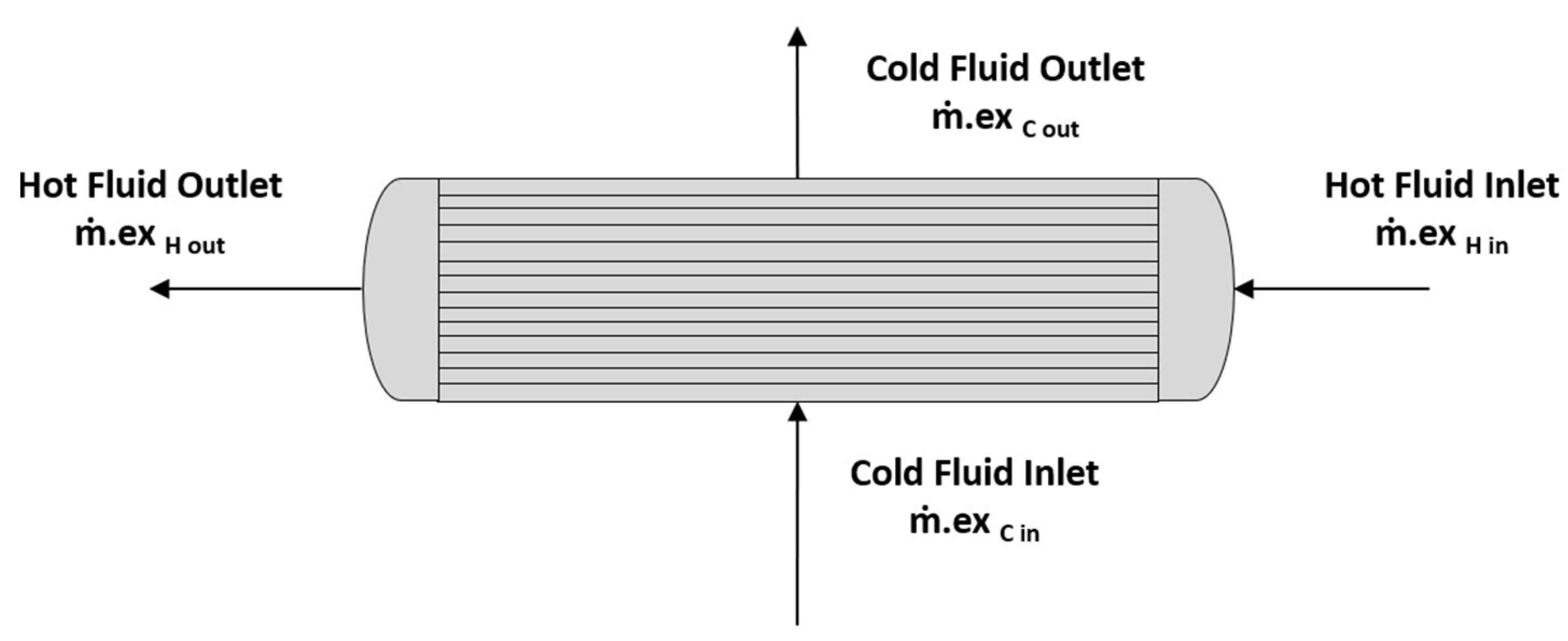
2.3.2. Heat Exchangers

Heat exchangers are devices that allow the transfer of heat between a cold stream (which will be heated or evaporated) and a hot stream (which will be cooled or condensed). The cycle exchangers are typically shell and tube type and the heat exchanged depends on the temperature difference between the incoming and outcoming streams. Figure 2 shows the exergy balance of a heat exchanger.

There are essentially two categories of heat exchangers in a refrigeration cycle: condensers (E-101 to E-105), which dissipate the heat absorbed by the users and generated by the fluid compression process in low temperature heat sources (cooling water and propylene refrigerant), and the evaporators (E-107 to E-116), which cool the process streams by absorbing the heat into the cycle. As an assumption, it is considered that there is no heat loss from the equipment to the environment, and thus the irreversibility is calculated by the difference between the exergy of the exchanger’s incoming and outgoing streams. Equation (8) shows the calculation of the irreversibility for these devices, where ṁ_H and ex_H are the mass flowrate and specific exergy of the hot stream, respectively, and ṁ_C and ex_C are the mass flow and the specific exergy of the cold stream.

$${\dot{\mathrm{I}}}_{\mathrm{HE}}=\left({\dot{\mathrm{m}}}_{\mathrm{H}}.{\mathrm{ex}}_{\mathrm{H} \mathrm{in}}+{\dot{\mathrm{m}}}_{\mathrm{C}}.{\mathrm{ex}}_{\mathrm{C} \mathrm{in}}\right)-\left({\dot{\mathrm{m}}}_{\mathrm{H}}.{\mathrm{ex}}_{\mathrm{H} \mathrm{out}}+{\dot{\mathrm{m}}}_{\mathrm{C}}.{\mathrm{ex}}_{\mathrm{C} \mathrm{out}}\right)$$

(8)

The exergy efficiency for heat exchangers is defined by the ratio between the increase in exergy on the cold side and the reduction in exergy of hot side [27], as shown Equation (9).

$${\mathsf{\Psi }}_{\begin{array}{c}\mathrm{exchangers}\\ \mathrm{T}>{\mathrm{T}}_0\end{array}}=\frac{{\dot{\mathrm{m}}}_{\mathrm{C}}\left({\mathrm{ex}}_{\mathrm{C} \mathrm{in}}-{\mathrm{ex}}_{\mathrm{C} \mathrm{out}} \right)}{{\dot{\mathrm{m}}}_{\mathrm{H}}\left({\mathrm{ex}}_{\mathrm{H} \mathrm{in}}-{\mathrm{ex}}_{\mathrm{H} \mathrm{out}} \right)}$$

(9)

It is observed that for heat exchangers where the operating temperature is higher than the reference temperature (T > T₀), there will indeed be an increase in the exergy of the cold side and a decrease in the hot side. In the cycle under evaluation, only the E-101 exchanger fits in this category because for the other exchangers, the operating temperature is lower than the reference temperature (T < T₀). In these cases, the exergy availability increases when there is heat loss; thus, the exergy of the hot side increases while the exergy of the cold side is reduced [27]. The exergy efficiency for these exchangers is then calculated by Equation (10), applied to all other refrigeration cycle exchangers, except for E-102.

$${\mathsf{\psi }}_{\begin{array}{c}\mathrm{exchangers}\\ \mathrm{T}<{\mathrm{T}}_0\end{array}}=\frac{{\dot{\mathrm{m}}}_{\mathrm{H}}\left({\mathrm{ex}}_{\mathrm{H} \mathrm{out}}-{\mathrm{ex}}_{\mathrm{H} \mathrm{in}} \right)}{{\dot{\mathrm{m}}}_{\mathrm{C}}\left({\mathrm{ex}}_{\mathrm{C} \mathrm{in}}-{\mathrm{ex}}_{\mathrm{C} \mathrm{out}} \right)}$$

(10)

The E-102 exchanger is in a transition zone, where the inlet of the hot side is above the ambient temperature, while the outlet is below. This makes Equations (9) and (10) provide negative results. For this exchanger, the classic concept of second law efficiency calculation proposed by Dincer and Rosen [26] was used, as observed in Equation (11).

$${\mathsf{\psi }}_{\mathrm{E}-102}=\frac{\left({\dot{\mathrm{m}}}_{\mathrm{H}}.{\mathrm{ex}}_{\mathrm{H} \mathrm{out}}+{\dot{\mathrm{m}}}_{\mathrm{C}}.{\mathrm{ex}}_{\mathrm{C} \mathrm{out}}\right)}{\left({\dot{\mathrm{m}}}_{\mathrm{H}}.{\mathrm{ex}}_{\mathrm{H} \mathrm{in}}+{\dot{\mathrm{m}}}_{\mathrm{C}}.{\mathrm{ex}}_{\mathrm{C} \mathrm{in}}\right)}$$

(11)

Both efficiency concepts presented by Wark [27] and Dincer and Rosen [26] are correct, and according to Mafi, Naeynian, and Amidpour [17], are commonly known as the “engineering approach” and the “scientific approach”, respectively, to calculate the second law efficiency. Both concepts were tested in this study, and it was found that the “engineering approach” of Wark [27] can better numerically distinguish the inefficiencies of each heat exchanger and therefore improves the comparison of the performance of these devices.

Another indicator used to monitor the performance of exchangers is the exergy destruction number (N_ex) proposed by Tirandazi et al. [14]. This indicator is calculated by the ratio between the exergy destroyed and the heat exchanged in the exchanger, according to Equation (12).

$${\mathrm{N}}_{\mathrm{ex}}=\frac{{\dot{\mathrm{I}}}_{\mathrm{HE}}}{\dot{\mathrm{Q}}}={\left(\frac{{\mathrm{ex}}_{\mathrm{in}}-{\mathrm{ex}}_{\mathrm{out}}}{{\mathrm{h}}_{\mathrm{in}}-{\mathrm{h}}_{\mathrm{out}}}\right)}_{\mathrm{C}}-{\left(\frac{{\mathrm{ex}}_{\mathrm{in}}-{\mathrm{ex}}_{\mathrm{out}}}{{\mathrm{h}}_{\mathrm{in}}-{\mathrm{h}}_{\mathrm{out}}}\right)}_{\mathrm{H}}$$

(12)

2.3.3. Control Valves and Lines

The control valves are devices where adiabatic expansion of the refrigerant fluid occurs. Since there is no work or heat generation or absorption in these devices, the calculation of irreversibility is defined by Equation (13). The second law efficiency is calculated by the ratio between the outgoing exergy and the incoming exergy in these devices, according to Equation (14).

$${\dot{\mathrm{I}}}_{\mathrm{Vc}}=\dot{\mathrm{m}}.{\mathrm{ex}}_{\mathrm{in}}-\dot{\mathrm{m}}.{\mathrm{ex}}_{\mathrm{out}}$$

(13)

$${\mathsf{\psi }}_{\mathrm{cv}}=\frac{\dot{\mathrm{m}}.{\mathrm{ex}}_{\mathrm{out}}}{\dot{\mathrm{m}}.{\mathrm{ex}}_{\mathrm{in}}}$$

(14)

The suction lines of the ethylene compressor (L1, L2, and L3) were included in the evaluation because they have a relevant pressure loss by design, which may affect cycle performance. Because they are isolated cryogenic lines, they were considered adiabatic, and therefore, the applicable equations are identical to the equations shown for the control valves.

2.3.4. Mixing Points

The mixing points represent locations in the process where several streams come together. If these streams have different temperatures, vapor fraction, or composition, the outlet stream will have a different condition from the inlet streams. Thus, the irreversibilities are calculated by the difference between the sum of exergy from the multiple inlet streams and the exergy of the outlet stream, as shown in Equation (15). The exergy efficiency is calculated by the ratio of the outlet stream exergy and the sum of the exergy of the input streams, according to Equation (16).

$${\dot{\mathrm{I}}}_{\mathrm{M}}={\displaystyle \sum }\dot{\mathrm{m}}.{\mathrm{ex}}_{\mathrm{in}}-\dot{\mathrm{m}}.{\mathrm{ex}}_{\mathrm{out}}$$

(15)

$${\mathsf{\psi }}_{\mathrm{M}}=\frac{\dot{\mathrm{m}}.{\mathrm{ex}}_{\mathrm{in}}}{{\displaystyle \sum }\dot{\mathrm{m}}.{\mathrm{ex}}_{\mathrm{out}}}$$

(16)

2.3.5. Vessels

Vessels are devices that allow the separation of the existing phases in the input stream. They are adiabatic devices without any type of work or heat interaction, so irreversibility is calculated by the difference between the exergy of the streams leaving the vessel and the input stream. This is shown in Equation (17), where ${\dot{\mathrm{m}}}_{\mathrm{V}+\mathrm{L}}.{\mathrm{ex}}_{\mathrm{V} + \mathrm{L}}$ are, respectively, the mass flowrate and specific exergy of the input stream and analogously, ṁ_V and ${\mathrm{ex}}_{\mathrm{V}}$ are the same variables of the vapor phase and ṁ_L ${\mathrm{ex}}_{\mathrm{L}}$ of the liquid phase. The efficiency for these devices is defined by Equation (18).

$${\dot{\mathrm{I}}}_{\mathrm{V}}={\dot{\mathrm{m}}}_{\mathrm{V}+\mathrm{L}}.{\mathrm{ex}}_{\mathrm{V}+\mathrm{L}}-{\dot{\mathrm{m}}}_{\mathrm{L}}.{\mathrm{ex}}_{\mathrm{L}}-{\dot{\mathrm{m}}}_{\mathrm{V}}.{\mathrm{ex}}_{\mathrm{V}}$$

(17)

$${\mathsf{\psi }}_{\mathrm{V}}=\frac{{\dot{\mathrm{m}}}_{\mathrm{L}}.{\mathrm{ex}}_{\mathrm{L}}+{\dot{\mathrm{m}}}_{\mathrm{V}}.{\mathrm{ex}}_{\mathrm{V}}}{{\dot{\mathrm{m}}}_{\mathrm{V}+\mathrm{L}}.{\mathrm{ex}}_{\mathrm{V}+\mathrm{L}}}$$

(18)

2.3.6. Refrigeration Cycle

The exergy efficiency of the refrigeration cycles is determined by the ratio between the power required if the process occurred reversibly (${\dot{\mathrm{W}}}_{\mathrm{rev}}$), which represents the minimum work rate required to drive the cycle, and the actual work (${\dot{\mathrm{W}}}_{\mathrm{actual}}$). The reversible work can be determined by the difference between the actual work rate and the sum of all irreversibilities that occur in the cycle [26]. The actual power of the refrigerant compressor can be measured or calculated using Equation (5). The calculation of exergy efficiency for refrigeration cycles is presented by Equation (19).

$$\mathsf{\psi }=\frac{{\dot{\mathrm{W}}}_{\mathrm{rev}}}{{\dot{\mathrm{W}}}_{\mathrm{actual}}}=\frac{{\dot{\mathrm{W}}}_{\mathrm{actual}}-{\dot{\mathrm{I}}}_{\mathrm{total}}}{{\dot{\mathrm{W}}}_{\mathrm{actual}}}$$

(19)

Another indicator that is commonly used to monitor the performance of refrigeration cycles is the coefficient of performance (COP), defined as the ratio between the total heat rate absorbed by the cycle (${\dot{\mathrm{Q}}}_{\mathrm{L}}$) and the actual power, shown by Equation (20). In addition, the specific energy consumption of the cycle (ξ) is another indicator typically applied to the monitoring of cycle performance, calculated by the ratio between the actual power and the circulating refrigerant flowrate (ṁ_ref), according to Equation (21). Both indicators are based only on the first law of thermodynamics.

$$\mathrm{COP}=\frac{{\dot{\mathrm{Q}}}_{\mathrm{L}}}{{\dot{\mathrm{W}}}_{\mathrm{actual}}}$$

(20)

$$\mathsf{\xi }=\frac{{\dot{\mathrm{W}}}_{\mathrm{actual}}}{{\dot{\mathrm{m}}}_{\mathrm{ref}}}$$

(21)

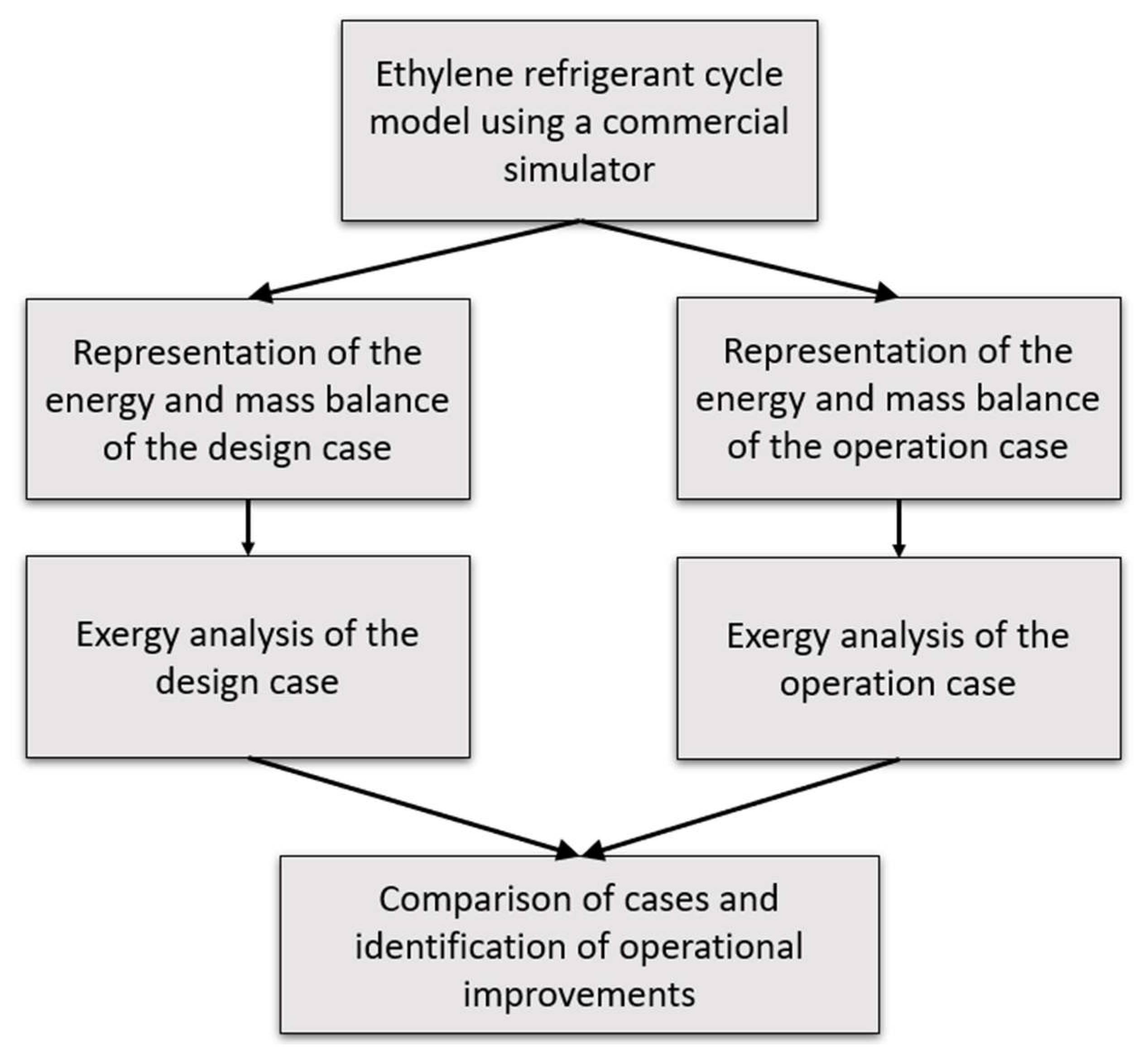
2.4. Methodological Approach

Two scenarios were chosen to perform the exergetic evaluation of the ethylene cycle:

• Design case: This case considers the mass and energy balance of the unit project, retrieved from the process design book. The performance curves of the compressor were regressed and used in the model to determine the theoretical operating conditions of the machine.
• Operation case: This case represents the current refrigerant cycle operational condition. A stable operating period was selected, that had similar throughput and process conditions to the design case. The data were collected, treated, and inputted in the model. In this scenario, the performance of the refrigerant compressor is calculated using the real operating data.

Table 1. Boundary conditions of the evaluated ethylene refrigeration cycle scenarios.

Description	Unit	Design	Operation
1st Stage Q users	MW	4.6	1.9
2nd Stage Q users	MW	4.1	3.9
3rd Stage Q users	MW	2.6	3.3
Q Coolers	MW	19.0	17.0
1st Stage Suction Pressure	kPa	103.3	103.3
2nd Stage Suction Pressure	kPa	331.8	319.0
3rd Stage Suction Pressure	kPa	844.6	760.3
Discharge Pressure	kPa	3004.1	2621.6
1st Stage Suction Temperature	°C	−102.0	−84.0
2nd Stage Suction Temperature	°C	−58.7	−49.0
3rd Stage Suction Temperature	°C	−19.9	−19.2
Discharge Temperature	°C	82.8	92.8

shows the main boundary conditions used in the simulation of the design and operation cases. The models were validated for both scenarios and had shown errors below 5% for all variables.

The exergetic evaluation of both scenarios requires two different sets of mass and energy balance and the comparison of results obtained assists the identification of process improvements. Figure 3 presents a flowchart with the proposed methodological approach.

3. Results and Discussion

The results obtained from the exergetic evaluation of the ethylene refrigeration cycle for the design and operation scenarios are presented. First, a detailed analysis of each set of previously described equipment is shown and after discussing the causes of the main differences found, an evaluation of the global indicators of the refrigeration cycle is presented.

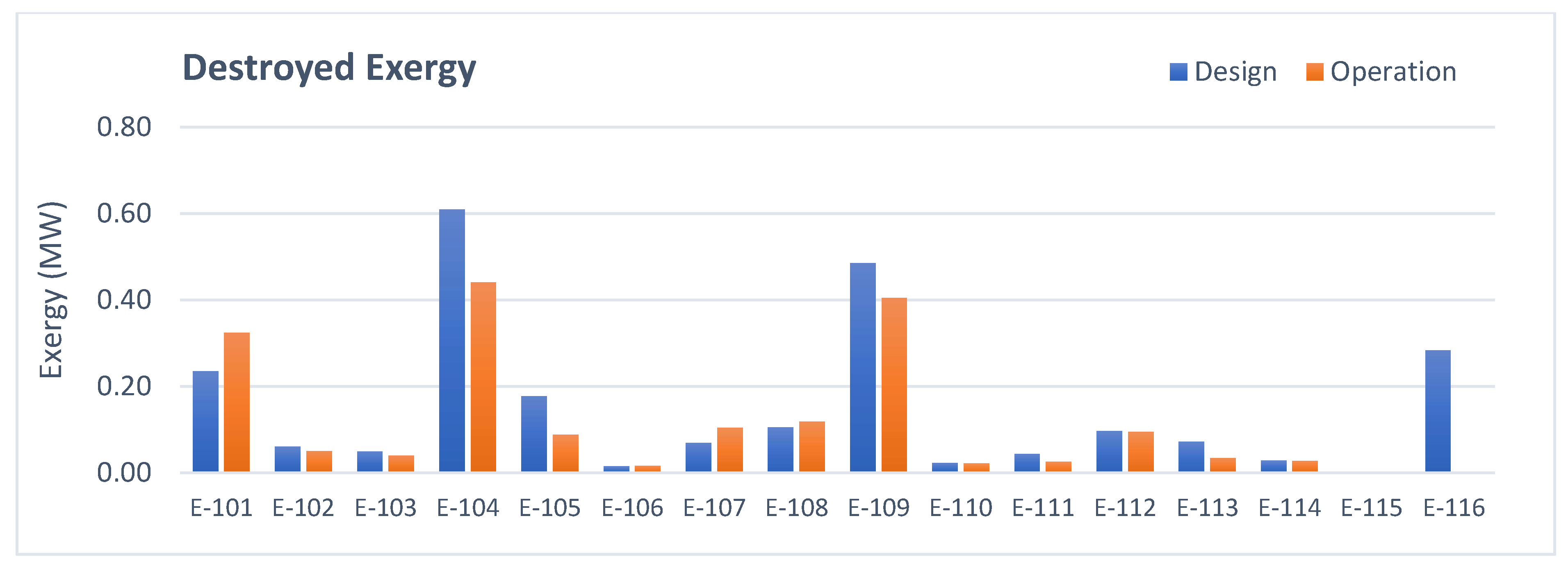
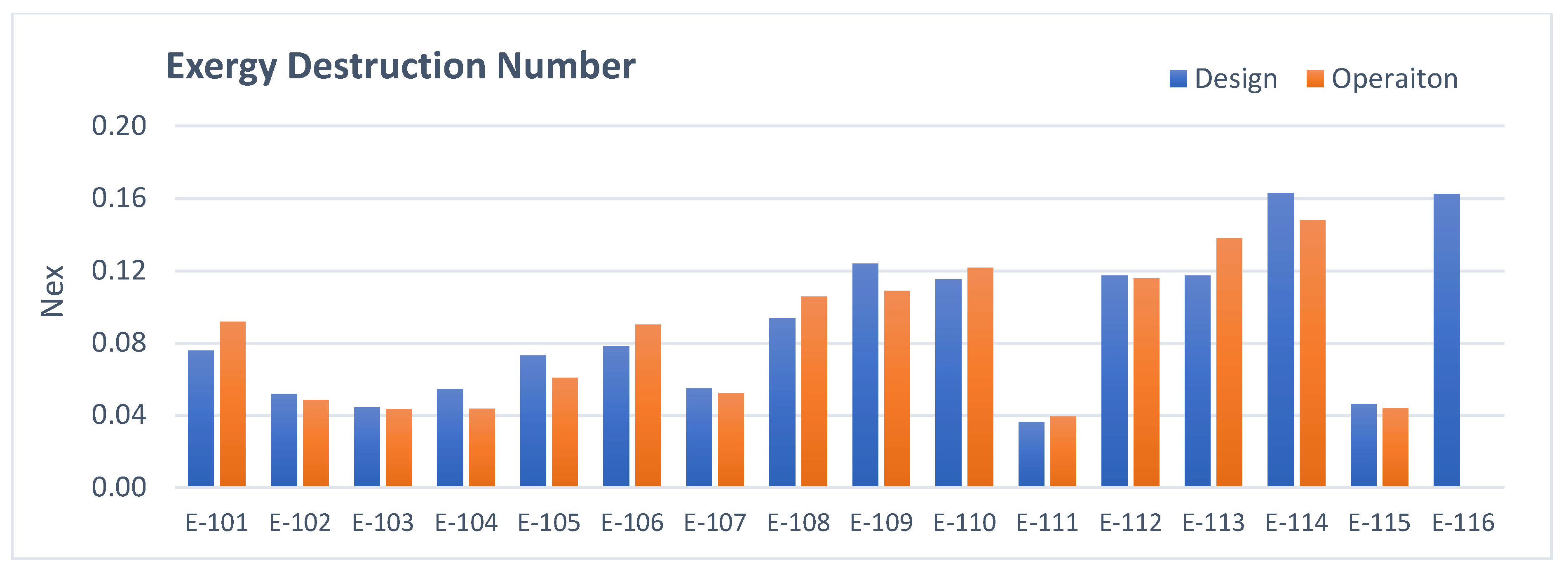
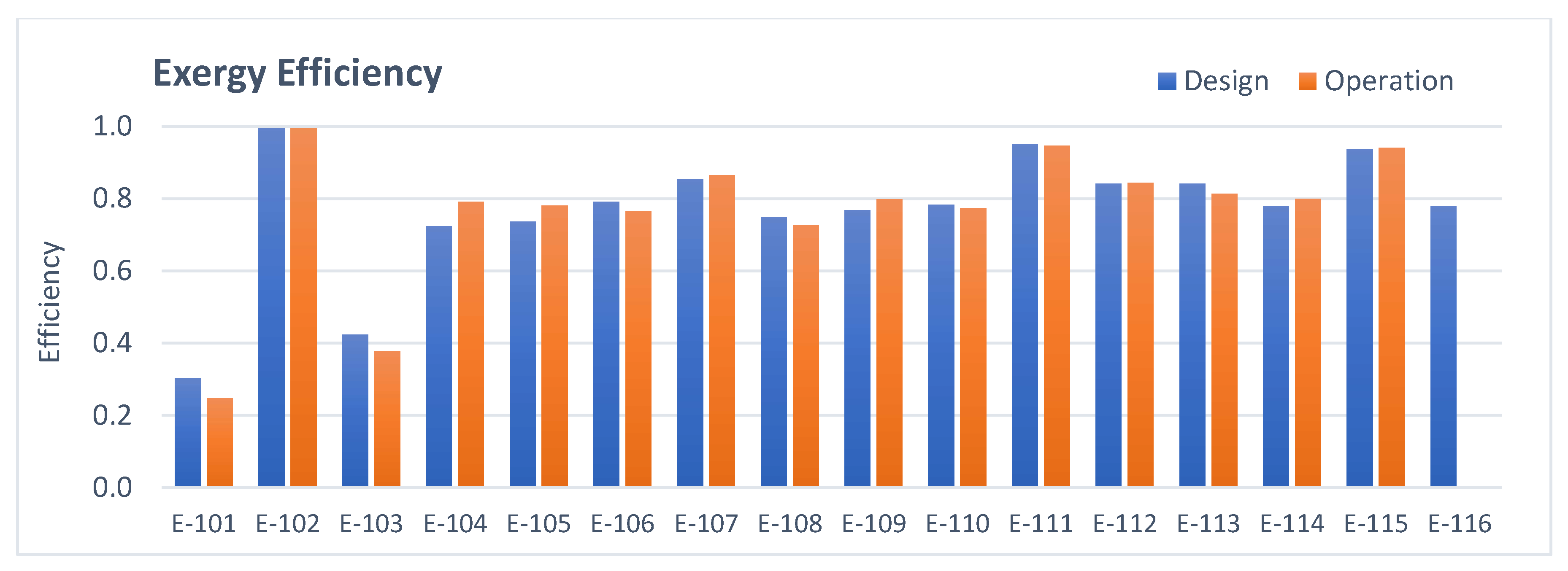
3.1. Heat Exchangers Analysis

Figure 4 shows the exergy destroyed in each of the cycle’s heat exchangers. The exergy destruction number and second law efficiency are shown in Figure 5 and Figure 6.

In general, most exchangers exhibit satisfactory performance in both evaluated cases, with exergy efficiencies close to 80%. Exchangers E-101 and E-103 have the lowest efficiency in the cycle. The efficiency of E-102 was calculated using the classical efficiency calculation approach, and therefore, higher values were observed compared to the other exchangers for both evaluated scenarios.

The E-101, E-104, E-109, and E-116 exchangers were the exchangers with the greatest amount of destroyed exergy, as well as the highest heat transfer rates, representing approximately 70% of all destroyed exergy in the cycle. A critical analysis of the results obtained for these devices are presented because of their relevance.

E-101 cools the ethylene coming out of the compressor discharge using cooling water, and due to the large temperature difference between the cold and hot sides, this is the exchanger with the lowest exergy efficiency. It is also the exchanger with the worst performance in the operation case compared to the design case, with 30% more exergy destroyed and 5% lower efficiency. The poor performance is mainly due to the higher discharge temperature of the third compressor stage (C-103). The greater the temperature difference between the cold and hot streams, the greater the generation of entropy in a heat exchanger.

E-104 is the ethylene refrigerant condenser and has the highest heat transfer rate of the entire cycle. It is also the heat exchanger with the greatest amount of destroyed exergy, although the exergy destruction number is one of the smallest in the cycle, which demonstrates that the irreversibility generated in this device is linked to its high heat transfer rate.

E-104 showed better performance in the operation case, with approximately 30% less exergy destruction and 7% greater exergy efficacy. The better operating condition is due to the lower condensed ethylene flowrate compared to the design case, which reduces the thermal load and the temperature differences in the exchanger because ethylene leaves the device with a higher subcooling degree.

E-109 is a condenser of the cryogenic separation unit, and like E-104, it has a better operating performance than in the design case. The lower exergy destruction results from a lower heat transfer rate and a slightly higher second law efficiency.

E-116 is a condenser in a distillation column of a unit that is stopped for commercial reasons; therefore, there is no consumption of ethylene refrigerant in the operation case. By design, this device requires a significant energy consumption of the refrigeration cycle, in addition to being the third largest source of irreversibility among the heat exchangers.

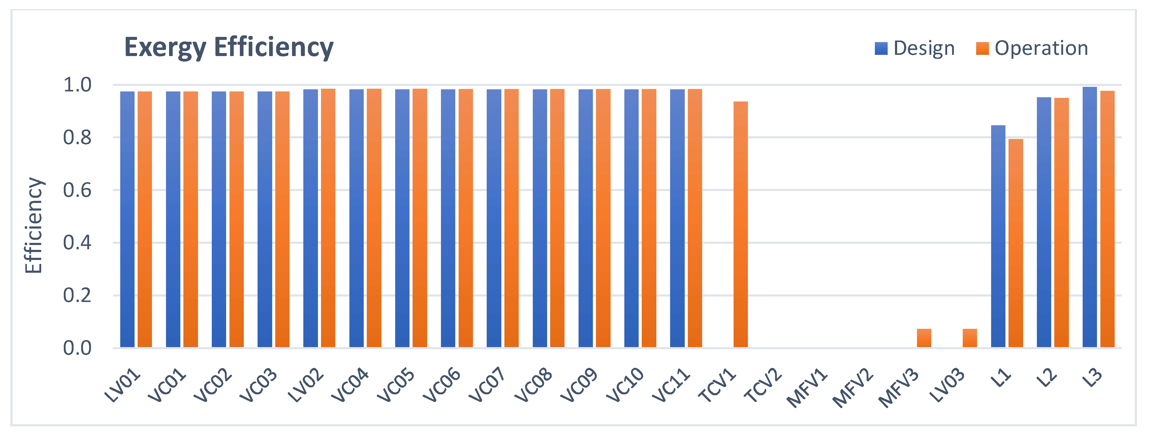
3.2. Valves and Lines Analysis

The exergy destroyed and the exergy efficiency of the valves and lines are presented in Figure 7 and Figure 8, respectively. Most of the refrigeration cycle valves have high efficiencies, with values close to 98%. The first stage mini-flow valve (MFV3) and the first stage level control valve (LV03) showed efficiencies below 10% in the operation case. Note that these valves were not predicted in the design case. The suction lines (L1 to L3) also showed high efficiencies, above 80% but had a low generation of irreversibilities.

Equation (13) shows that the amount of exergy destroyed in the control valves is directly linked to the flowrate of this device. In the evaluation of the cycle in question, the process conditions (temperature and pressure) in both scenarios are similar, so that the specific exergy does not change significantly. Thus, the difference in flowrate between the two evaluated cases appears to be the main cause for the difference in exergy destroyed in these devices.

Despite having a high exergy efficiency, the third stage level control valve (LV-01) has a significant exergy destruction of 0.24 MW. The explanation lies in the high ethylene flowrate through this valve, which represents approximately 75% of the entire flowrate of the cycle. In the operation case, this valve generates approximately 70% less irreversibilities because it also processes a 70% lower flowrate.

The largest portion of exergy destruction in the valves and lines (approximately 65%) occurs because of the operation of the mini-flow valves (MFV3) and the first stage level control valve (LV03) in the operation case.

Exchanger E-116 is currently out of operation. In the design case, this exchanger processes approximately 35% of the entire ethylene flowrate of the first refrigeration stage. With the removal of this exchanger from operation, there is a reduction in the suction flowrate that causes the machine to operate close to its surge limit. The anti-surge control of the compressor drives the MFV1 valve, which then operates continuously to increase the flowrate in the first stage.

Anti-surge protection control exists to ensure the mechanical integrity of the compressor; however, it reduces cycle efficiency. The ethylene flowrate that starts to circulate to maintain the reliability of the machine consumes part of the compression energy, but this portion is not converted into refrigeration and is rather wasted by the pressure reduction that occurs in the mini-flow valves. This explains the generation of irreversibilities observed in the MFV1 valve, and consequently, its low exergy efficiency.

The continuous use of mini-flow in the first stage also makes it necessary to manipulate the temperature control valve (TCV1) and also the valve that regulates the first stage level (LV03). While TCV1 has an efficiency greater than 90% and a small amount of exergy destroyed, LV03 has the same efficiency as the MFV1 valve, because they have the same input and output conditions. Adding the exergy destroyed by these three valves, it can be stated that the continuous use of mini-flow causes the destruction of approximately 1.2 MW of exergy destruction in the operation case.

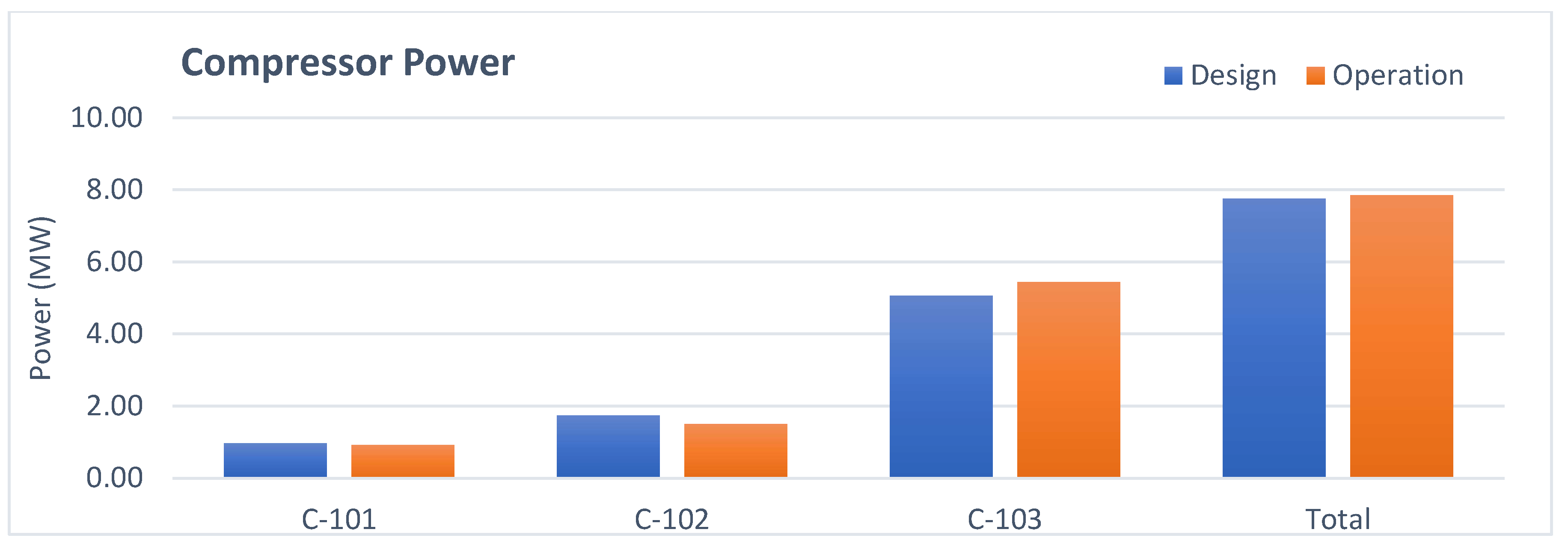
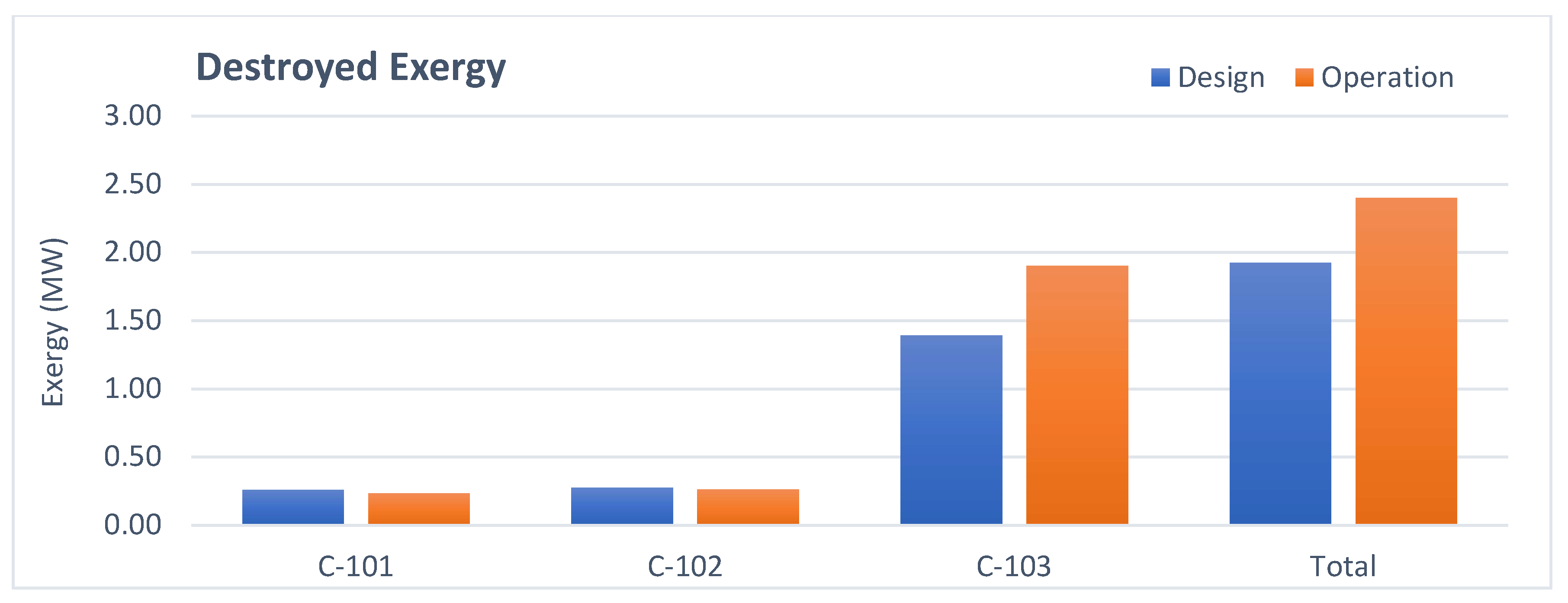
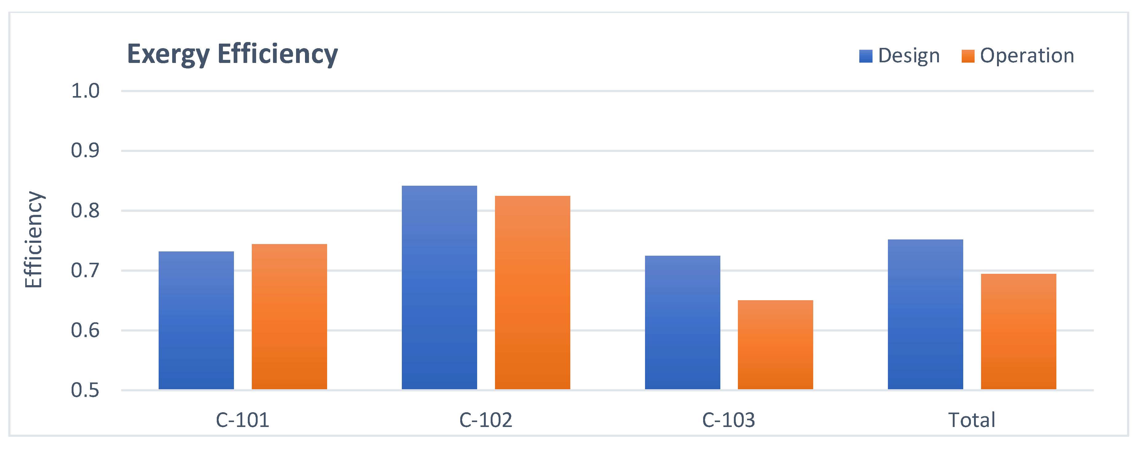
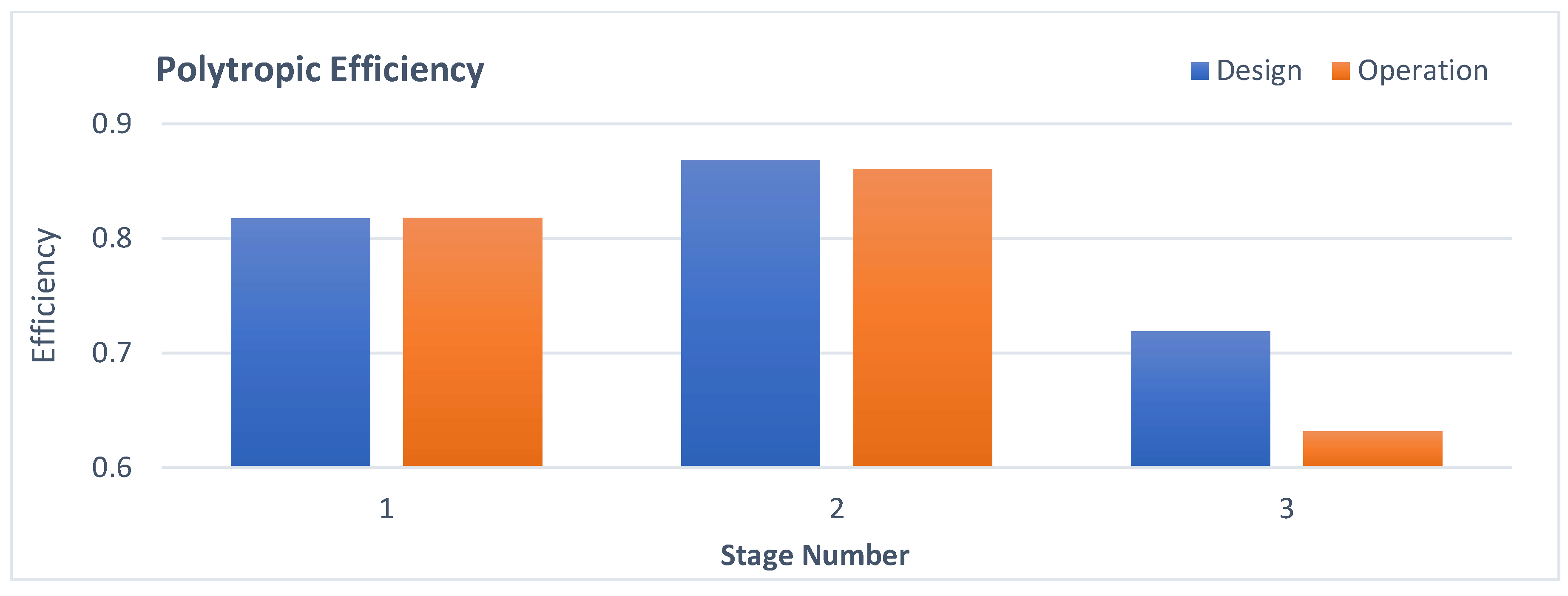
3.3. Refrigerant Compressor Analysis

Figure 9 shows the energy consumption of the refrigerant compressor, while Figure 10, Figure 11 and Figure 12 show the exergy destroyed, the second law efficiency and the polytropic efficiency of each compression stage, respectively. For both evaluated cases, the third stage generates the largest amount of irreversibilities and has the lowest exergy efficiency. There are two reasons for this observation: the third stage of the machine is the section with the lowest polytropic efficiency and the highest compression power (representing approximately 65% of the energy consumption of the compressor) for both evaluated scenarios.

Evaluation of the compressor results shows that the energy demand is similar between the operation and design cases but the amount of exergy destroyed in operation is 25% higher, resulting from a lower polytropic efficiency. As observed in Figure 12, the third stage has an operating polytropic efficiency lower than predicted by design. It should be noted that to calculate the polytropic efficiency of an operating compressor, it is necessary to measure its discharge temperature, which cannot be done for the first and second stages because there are no internal temperature measurements in the machine. The third stage is the only stage that has temperature measurement at discharge and it is the only stage that the actual polytropic efficiency can be calculated, while the efficiency of the other stages is determined by the performance curve. In summary, because of the unavailability of temperature measurements inside the compressor, the value calculated for the polytropic efficiency of the third stage can allocate the inefficiencies of the other stages. Despite this limitation in the calculation, the compressor has a lower operating efficiency compared to the projected values.

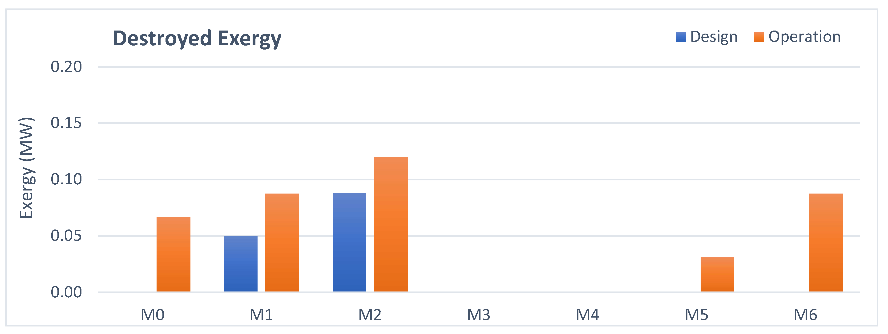
3.4. Mixing Points Analysis

The mixing points are treated as direct contact heat exchangers, and the greater the temperature difference between the streams to be mixed, the greater the exergy destroyed.

There are seven mixing points in the refrigeration cycle under evaluation that are presented in

Table 2. Mixing points of the ethylene refrigeration cycle.

Name	Process Point
M0	C-101 Suction
M1	C-102 Suction
M2	C-103 Suction
M3	V-102 Inlet
M4	V-103 Inlet
M5	V-104 Inlet
M6	V-104 Vaporization Point

, which lists their respective locations in the process and their respective names. The mixing points are also shown in Figure 1.

Figure 13 and Figure 14 show, respectively, the amount of exergy destroyed and the second law efficiency calculated for the mixing points of the ethylene refrigeration cycle. Note that in the design case, only the mixing points of the suction of the second and third stages of the refrigerant compressor show the generation of irreversibilities because these are the points where there is a difference in the temperature of the ethylene gas, since the gas phases of the interstage vessels cool the discharge from the previous stage. Despite this, the amount of exergy destroyed is small, and the second law efficiency is greater than 98%. For the operation case, all the mixing points show exergy destruction, apart from the mixing points of the ethylene vaporized by the users (M3 and M4).

Analysis of the data indicates that operating with the first stage mini-flow valve continuously open is the main reason for the higher generation of irreversibilities in the mixing points because of the overheating of the ethylene in this section of the process.

Both the first stage mini-flow valve (MFV3) and the valve that controls the level of the first stage (LV03) use ethylene gas from the outlet of the E-103 cooler, which is at −28 °C after pressure reduction. The mixture of these streams with ethylene vaporized by the first stage users (which is at the saturation temperature) causes overheating of the ethylene from the suction of the first compression stage. The first stage temperature control valve (TCV1) should be actuated to reduce the degree of ethylene overheating. Currently, this temperature control is not operating in automatic mode, which means that this valve is being actuated manually. This occurs because there is a significant amount of liquid ethylene after pressure reduction (approximately 20% liquid) and a sudden variation in the control can cause a liquid carryover into the machine, which may cause actuation of the compressor interlock system due to high level in the first stage suction vessel (V-104).

Another issue observed was the difference in the temperature value of the produced ethylene storage tank boil-off stream. By design, the expected temperature value was −100 °C, while in operation, the actual temperature operates at approximately 45 °C. It was found that there was an error in the design when considering a temperature of −100 °C for this stream since it exits the discharge of a reciprocating compressor, whose projected temperature is similar to the value observed in operation.

Thus, mixing these different streams with different temperatures and vapor fraction is the reason for the greater generation of irreversibilities and the lower efficiency of the M0, M5, and M6 mixing points in the operation case.

Because of the aforementioned reasons, the ethylene in the first stage suction has approximately 20 °C of overheating, which causes an increase in the energy consumption of the compressor due to the increase in the volumetric flowrate of the gas at suction, increase of the ethylene temperature at the discharge of each stage, and the increase of exergy destruction in the M1 and M2 mixing points and of the E-101 exchanger.

3.5. Vessels Analysis

None of the vessels (V-101 to V-104) generated irreversibilities in either evaluated case. This is because all vessels were considered adiabatic processes with negligible head loss, where only the separation of the liquid and vapor phases of the feed stream occurs. Other authors reached the same conclusion [14,17,18].

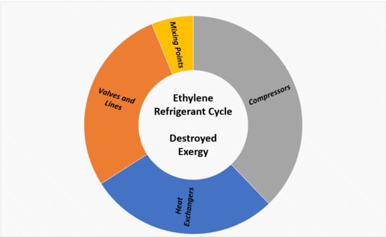
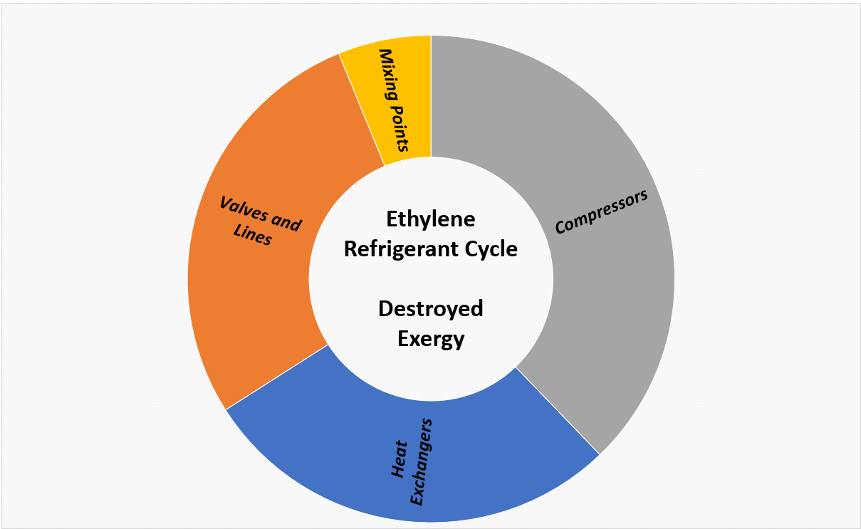
3.6. Refrigeration Cycle Analysis

Figure 15 shows the total amount of exergy destroyed per type of device in the cycle. The amount of irreversibilities generated in operation is 22% higher than that predicted in the design.

The explanations for the difference found in the exergy balance between the evaluated scenarios are presented in the specific sections corresponding to each device, which can be summarized as follows:

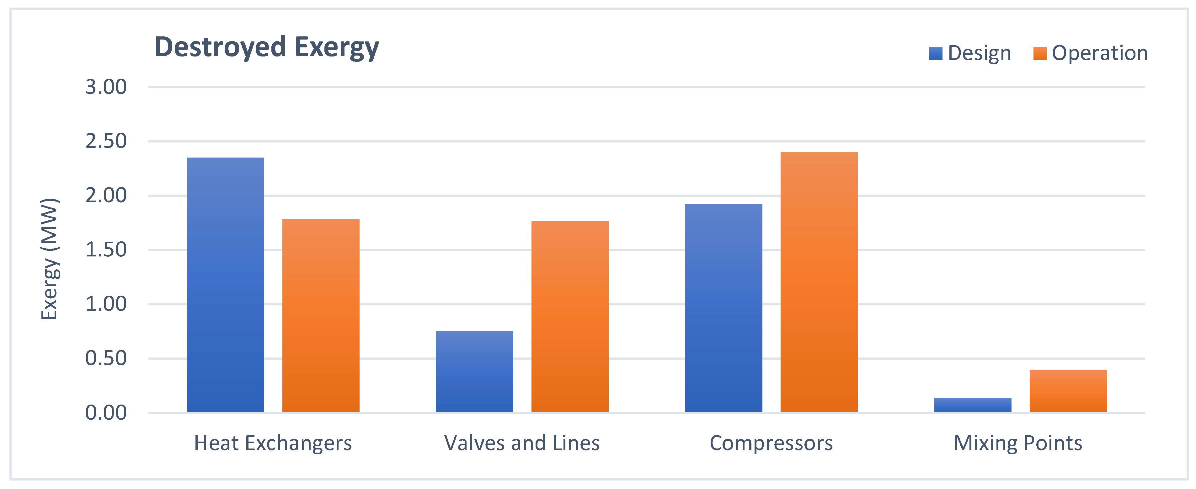
• Heat exchangers: The total amount of irreversibilities is lower in operation mainly due to the lower energy consumption of the users and removal of E-116 from operation.
• Valves and lines: The higher amount of irreversibilities generated in operation is due to the action of the mini-flow valve (MFV3) and first stage level control valve.
• Compressor: The higher exergy destruction in operation is due to a lower polytropic efficiency.
• Mixing points: The higher exergy destruction in operation is due to the greater temperature difference between the streams at the suction of the first stage.

A summary of the performance indicators calculated for the ethylene refrigeration cycle is presented in

Table 3. Summary of the refrigeration cycle performance indicators.

Indicator	Type	Unit	Design	Operation	Variation
Specific energy consumption	1st Law	kJ.kg−1	217.5	233.6	7.4%
COP	1st Law	-	1.45	1.16	−20.0%
Reversible work	2nd Law	MW	2.59	1.51	−41.8%
2nd law efficiency	2nd Law	-	0.33	0.19	−42.5%

. All calculated indicators confirm the worst performance of the cycle in the operation case, but each indicator has a different relative variation.

Specific energy consumption is the only indicator that does not have a thermodynamic basis, being only a direct relationship between energy consumption and the flowrate of ethylene that circulates in the cycle. It is considered an indirect indicator of efficiency, and according to Table 3, this indicator has the lowest percentage variation.

COP represents the first law of thermodynamic efficiency of the refrigeration cycles, according to (20). This indicator is calculated based on the energy required to vaporize ethylene at each refrigeration stage, while the specific energy consumption only makes a correlation between the power and the circulating refrigerant flowrate. The amount of energy required to vaporize the same mass of ethylene increases with the reduction of the pressure of each refrigeration stage, and for this reason, the COP can better represent the cycle performance because it considers the different energy levels at each stage. In this case, the variation of the COP is higher than that of the specific energy consumption.

Table 3 also shows the performance indicators based on the second law of thermodynamics. The reversible work of the cycle in operation has a lower value than the design case, because of the greater amount of exergy destroyed. The second law efficiency of the cycle is affected by the greater amount of irreversibilities generated and the higher energy consumption by the refrigerating compressor in the operation case. The second law indicators are determined from the exergy balance of the cycle and therefore consider the variations in enthalpy and entropy generation in the process. Table 3 shows that there is a greater variation in the value of these indicators when compared to the first law indicators. It is possible to conclude that when the variation in energy quantity and quality throughout the cycle is considered in the analysis, the performance difference between the evaluated cases is even greater.

3.7. Identified Opportunities for Refrigeration Cycle Performance Improvement

Two major opportunities to improve the refrigeration cycle performance were identified by comparing the simulation results of the design and operation cases:

• Refrigerant compressor efficiency recovery, whose value is below that predicted by the compressor performance curve. This can be achieved by performing general maintenance of this equipment in the next equipment turnaround.
• Closure of the first refrigeration stage mini-flow valve, through a better flow distribution among the TCV1, LV03, and MFV3 valves. With the removal of the E-116 exchanger from operation, it is necessary to maintain a recirculating flow to the first stage to ensure that the compressor does not operate close to the surge point. Currently, much of this circulation is performed by the anti-surge control valve, which causes ethylene to overheat at the compressor’s first stage suction. The use of the TCV1 and LV03 valves can increase the ethylene recirculation in the first stage to the point that it is no longer necessary to operate with the mini-flow valve open, which reduces the first stage suction temperature to values near to the saturation point.
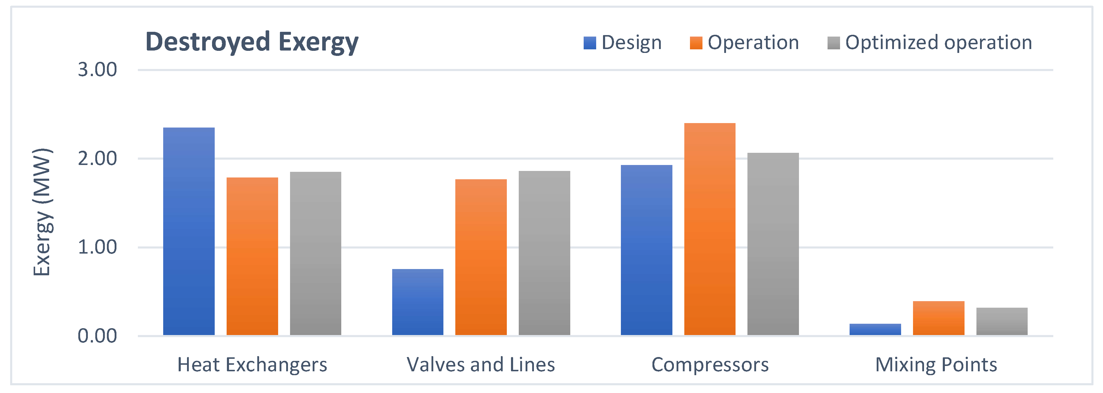
• A third case (optimized operation) was simulated considering the implementation of the two identified opportunities. Figure 16 shows a comparison of the amount of exergy destroyed per device type for the operation case and for the optimized operation case. There was a reduction of approximately 4% in the total amount of exergy destroyed in the new case evaluated because of the better performance of the refrigerant compressor and the lower generation of irreversibilities at the mixing points.

Table 4. Summary of refrigeration cycle performance indicators.

Indicator	Unit	Design	Operation	Optimized Operation
Specific energy consumption	kJ.kg−1	217.5	233.6	224.9
COP	-	1.45	1.16	1.19
Reversible work	MW	2.59	1.51	1.56
2nd law efficiency	-	0.33	0.19	0.20
Compressor power	MW	7.76	7.85	7.66

presents a comparison of cycle performance indicators for all evaluated scenarios. An improvement in these indicators is observed for the new case when comparing it with the operation case. It shows an approximate reduction of 0.20 MW in energy consumption of the refrigerant compressor, which represents a 2.5% reduction in the total consumed power.

The better distribution of the first stage circulation flowrate among the TCV1, LV03, and MFV3 valves minimizes the amount of exergy destroyed in the mixing points, because of the reduction in the first stage suction temperature and subsequent decrease in the discharge temperature of the other stages. However, when analyzing the amount of exergy destroyed by the recycle valves, it was found that the number of irreversibilities generated increased by 3%, because of the increase of exergy destroyed by the level control valve of the first stage drum (LV3). This shows that sustaining a minimum flow to compensate for the flow reduction, caused by the removal of one of the main users of the first stage, remains as the main cause of inefficiency in this refrigeration cycle.

4. Conclusions and Future Work

The present study aimed to identify opportunities for reducing the energy consumption of an ethylene refrigeration cycle of an existing petrochemical plant by conducting an exergetic evaluation of this process in two scenarios and comparing their results: a design case, which represents how the plant was designed to operate, and an operation case, which describes the current operational cycle condition.

The study showed that the amount of irreversibilities generated in operation is 22% above the predicted value in the design. It was identified that the removal from operation of a heat exchanger resulted in operation at a higher recycle flowrate to the first stage, ensuring the refrigerant compressor reliability. Additionally, it was also found that the refrigerant compressor has a lower operating polytropic efficiency than that projected. For these reasons, the values calculated for the second law cycle indicators in operation are approximately 40% below that projected.

To quantify the impact of implementing the identified improvement opportunities, a third scenario was simulated using the same simulation model developed for the cycle. There is a potential reduction of approximately 2.5% of the cycle’s energy consumption, so it is recommended to implement the identified improvements.

The authors also recommend the following future work, based on the knowledge acquired: conduct a complete advanced exergetic analysis of the combined cycles of ethylene and propylene refrigerant of an olefins plant, identifying the avoidable and unavoidable exergy destruction. Also, apply the concepts of thermo-economy and perform the optimization of the main users of the refrigeration cycles, assessing the possible improvements in the process and the refrigerant side.

References

1. Matar, S.; Hatch, L.F. Chemistry of Petrochemical Process, 2nd ed.; Gulf Publishing Company: Houston, TX, USA, 2001. [Google Scholar]
2. Pickett, T.M. Refrigeration Technology as Practiced in Olefins Plants. AIChE Spring Natl. Meet. 2005. Available online: https://epc.omnibooksonline.com/65235-epc-2005a-1.3718294/t008-1.3718512/f008-1.3718513/a031-1.3718523/ap031-1.3718524 (accessed on 10 April 2020).
3. Fuentes, A. Brasil Piora em Ranking e Passa a ser o 6° com a Energia Mais Cara do Mundo. Available online: https://veja.abril.com.br/blog/impavido-colosso/brasil-piora-em-ranking-e-passa-a-ser-o-6-com-a-energia-mais-cara-do-mundo/ (accessed on 10 April 2020).
4. Pfenninger, S.; Hawkes, A.; Keirstead, J. Energy systems modeling for twenty-first century energy challenges. Renew. Sustain. Energy Rev. 2014, 33, 74–86. [Google Scholar] [CrossRef]
5. Zhou, N.; Fridley, D.; Khanna, N.Z.; Ke, J.; McNeil, M.; Levine, M. China’s energy and emissions outlook to 2050: Perspectives from bottom-up energy end-use model. Energy Policy 2013, 53, 51–62. [Google Scholar] [CrossRef]
6. Catalán-Gil, J.; Sánchez, D.; Llopis, R.; Nebot-Andrés, L.; Cabello, R. Energy evaluation of multiple stage commercial refrigeration architectures adapted to F-gas regulation. Energies 2018, 11, 1915. [Google Scholar] [CrossRef] [Green Version]
7. Rivero, R. Application of the exergy concept in the petroleum refining and petrochemical industry. Energy Convers. Manag. 2002, 43, 1199–1220. [Google Scholar] [CrossRef]
8. Tsatsaronis, G. Recent developments in exergy analysis and exergoeconomics. Int. J. Exergy 2008, 5, 489. [Google Scholar] [CrossRef]
9. Zhang, Z.; Hou, Y.; Kulacki, F.A. Energetic and exergetic analysis of a transcritical N2O refrigeration cycle with an expander. Entropy 2018, 20, 31. [Google Scholar] [CrossRef] [Green Version]
10. Dokandari, D.A.; Mahmoudi, S.M.S.; Bidi, M.; Khoshkhoo, R.H.; Rosen, M.A. First and second law analyses of trans-critical N2O refrigeration cycle using an ejector. Sustainability 2018, 10, 1177. [Google Scholar] [CrossRef] [Green Version]
11. Gullo, P. Advanced thermodynamic analysis of a transcritical R744 booster refrigerating unit with dedicated mechanical subcooling. Energies 2018, 11, 3058. [Google Scholar] [CrossRef] [Green Version]
12. Ahamed, J.U.; Saidur, R.; Masjuki, H.H. A review on exergy analysis of vapor compression refrigeration system. Renew. Sustain. Energy Rev. 2011, 15, 1593–1600. [Google Scholar] [CrossRef]
13. Jahromi, F.S.; Beheshti, M.; Rajabi, R.F. Comparison between differential evolution algorithms and response surface methodology in ethylene plant optimization based on an extended combined energy—Exergy analysis. Energy 2018, 164, 1114–1134. [Google Scholar] [CrossRef]
14. Tirandazi, B.; Mehrpooya, M.; Vatani, A.; Moosavian, S.M.M.A.A. Exergy analysis of C2+ recovery plants refrigeration cycles. Chem. Eng. Res. Des. 2011, 89, 676–689. [Google Scholar] [CrossRef]
15. Lobosco, R.J. Análise do Desempenho Termodinâmico e Ambiental de um ciclo de Refrigeração e Proposta de uma Função Global de Avaliação. Doctoral Dissertation, Universidade Estadual de Campinas, Campinas, Brazil, 2009. [Google Scholar]
16. Sivakumar, M.; Somasundaram, P. Exergy and energy analysis of three stage auto refrigerating cascade system using Zeotropic mixture for sustainable development. Energy Convers. Manag. 2014, 84, 589–596. [Google Scholar] [CrossRef]
17. Mafi, M.; Naeynian, S.M.M.; Amidpour, M. Exergy analysis of multistage cascade low temperature refrigeration systems used in olefin plants. Int. J. Refrig. 2009, 32, 279–294. [Google Scholar] [CrossRef]
18. Fábrega, F.M.; Rossi, J.S.; D’Angelo, J.V.H. Exergetic analysis of the refrigeration system in ethylene and propylene production process. Energy 2010, 35, 1224–1231. [Google Scholar] [CrossRef]
19. Mahabadipour, H.; Ghaebi, H. Development and comparison of two expander cycles used in refrigeration system of olefin plant based on exergy analysis. Appl. Therm. Eng. 2013, 50, 771–780. [Google Scholar] [CrossRef]
20. Ghannadzadeh, A.; Sadeqzadeh, M. Exergy analysis as a scoping tool for cleaner production of chemicals: A case study of an ethylene production process. J. Clean. Prod. 2015, 129, 508–520. [Google Scholar] [CrossRef]
21. Vilarinho, A.N.; Campos, J.B.L.M.; Pinho, C. Energy and exergy analysis of an aromatics plant. Case Stud. Therm. Eng. 2016, 8, 115–127. [Google Scholar] [CrossRef] [Green Version]
22. Palizdar, A.; Sadrameli, S.M. Conventional and advanced exergoeconomic analyses applied to ethylene refrigeration system of an existing olefin plant. Energy Convers. Manag. 2017, 138, 474–485. [Google Scholar] [CrossRef]
23. Harvey, S. Centrifugal compressors in ethylene plants. Chem. Eng. Prog. 2017, 113, 28–32. [Google Scholar]
24. Schaider, L.; Desai, P. Trends in Monitoring and Control of Ethylene Plant Compressors. AIChE Ethyl. Prod. Conf. Proc. 2002, 23. [Google Scholar]
25. Brown, J.S. Predicting performance of refrigerants using the Peng-Robinson Equation of State. Int. J. Refrig. 2007, 30, 1319–1328. [Google Scholar] [CrossRef]
26. Dincer, I.; Rosen, M.A. EXERGY: Energy, Environment and Sustainable Development; Elsevier: Amsterdam, The Netherlands, 2007; ISBN 0080531350. [Google Scholar]
27. Wark, K.J. Advanced Thermodynamics for Engineers; McGraw-Hill: New York, NY, USA, 1995. [Google Scholar]
28. Montanez-Morantes, M.; Jobson, M.; Zhang, N. Operational optimisation of centrifugal compressors in multilevel refrigeration cycles. Comput. Chem. Eng. 2016, 85, 188–201. [Google Scholar] [CrossRef]
Figure 1. Process scheme of the ethylene refrigeration cycle.
Energies 13 03753 g001
Figure 2. Exergy balance of a heat exchanger.
Energies 13 03753 g002
Figure 3. Methodological approach for exergetic evaluation of the ethylene refrigerant cycle.
Energies 13 03753 g003
Figure 4. Exergy destroyed by the heat exchangers.
Energies 13 03753 g004
Figure 5. Exergy destruction number of heat exchangers.
Energies 13 03753 g005
Figure 6. Exergy destruction number of heat exchangers.
Energies 13 03753 g006
Figure 7. Exergy destroyed by valves and lines.
Energies 13 03753 g007
Figure 8. Exergy efficiency of valves and lines.
Energies 13 03753 g008
Figure 9. Power consumption of the refrigerant compressor.
Energies 13 03753 g009
Figure 10. Exergy destroyed by the refrigerant compressor.
Energies 13 03753 g010
Figure 11. Exergy efficiency of each refrigerant compressor stage.
Energies 13 03753 g011
Figure 12. Polytropic efficiency of the refrigerant compressor.
Energies 13 03753 g012
Figure 13. Amount of exergy destroyed by the mixing points.
Energies 13 03753 g013
Figure 14. Exergy efficiency of the mixing points.
Energies 13 03753 g014
Figure 15. Amount of exergy destroyed per device type.
Energies 13 03753 g015
Figure 16. Exergy destroyed by type of device for the optimized operation case.
Energies 13 03753 g016