Assessment of Hybrid RANS/LES Models in Heat and Fluid Flows around Staggered Pin-Fin Arrays

Abstract

In the present work, the three-dimensional heat and fluid flows around staggered pin-fin arrays are predicted using two hybrid RANS/LES models (an improved delayed detached eddy simulation (IDDES) model and a stress-blended eddy simulation (SBES) model), and one transitional unsteady Reynolds averaged Navier-Stokes (URANS) model, called k-ω SSTLM. The periodic segment geometry with a total of nine pins is considered with a channel height of 2D and a distance of 2.5D between each pin. The corresponding Reynolds number based on the pin diameter and the maximum velocity between pins is 10,000. The two hybrid RANS/LES results show the superior prediction of the mean velocity profiles around the pins, pressure distributions on the pin wall, and Nusselt number distributions. However, the transitional model, k-ω SSTLM, shows large discrepancies except in front of the pins where the flow is not fully developed. The vortical structures are well resolved by the two hybrid RANS/LES models. The SBES model is particularly adept at capturing the 3-D vortex structures after the pins. The effects of the blending function switching between RANS and LES mode of the two hybrid RANS/LES models are also investigated.

1. Introduction

The pin-fin structures utilized in heat exchangers, nuclear reactors, and turbine-bladed cooling systems are a common method to enhance heat transfer efficiently. Even though its geometry is relatively simple, the structure of fluid and heat transfer is known to be complex. Therefore, many experimental and numerical types of research have been conducted to evaluate the performance of pin-fin geometry and to elucidate the fluid and heat transfer mechanism around pin-fin structures [1]. Recently, the phenomenon with forced convective heat transfer in these kinds of geometry has been interested in the research not only at the microscale but also at the nanoscale [2,3].

Ames et al. [4,5,6] conducted an experiment to study the heat transfer and fluid dynamics of staggered pin-fin arrays using a hot wire measurement and an infrared camera at Reynolds numbers 3000, 10,000, and 30,000 based on the maximum velocity between the pins. Pressure coefficient distributions, velocity distributions, and Nusselt number distributions were acquired near the cylindrical pins and off the end-walls. Their experimental results showed that the turbulence augmentation along the rows were a major parameter for heat transfer in a staggered pin-fin array, and their averaged end-wall Nusselt number had a good agreement with Metzger and Haley’s correlation and Van Fossen’s correlations. Ames et al. [5] also applied computational fluid dynamics (CFD) simulations with 3-D steady k-ε turbulence model series (standard, renormalization group (RNG), realizable) on the same configuration. They showed the limitations of steady k-ε turbulence models which failed to capture the unsteady vortex shedding in staggered pin-fin arrays.

Delibra et al. [7,8,9] conducted CFD simulations with three kinds of turbulence models at two different Reynolds numbers, 10,000 and 30,000. The three turbulence models were an unsteady Reynolds-averaged Navier-Stokes (URANS) model called the ζ-f model, a dynamic Smagorinsky subgrid-scale large eddy simulation (LES) model, and a hybrid LES/RANS model combined with the ζ-f model and the dynamic Smagorinsky subgrid-scale LES model. The ζ-f model was able to capture the unsteady flow features caused by vortex shedding. However, like the LES model, it showed discrepancies in resolving the wake’s size and structure behind the first pin. Considering the heat transfer, the averaged end-wall Nusselt number of the ζ-f model was close to the results of the LES, but both values were underpredicted to the experimental results. Although a hybrid LES/RANS model used the same grid as the URANS simulation, the results showed relatively better agreement than the URANS results with LES and the experimental results.

A study by Hao and Gorle [10] adopted a pin-fin array based on LES and a k-ω SST model to perform an a priori examination of a selected RANS model considering discrepancies of the Reynolds stress tensor. Their wall-resolving LES results showed good agreement with experimental data, including mean velocity, Reynolds shear stress, and local averaged Nusselt number. They also found that the linear eddy viscosity model of RANS is inadequate in complex engineering problems such as pin-fin arrays, and provided insight on correcting the shape of the Reynolds stress tensor through reference data from the LES.

The stochastic method for heat transfer prediction based on LES and steady RANS was applied to a duct flow with pin-fin arrays by Carnevale et al. [11] The Reynolds number was considered as a random variable with a normal distribution. The results of LES showed the probability of a specified heat loading under a probabilistic condition. However, the results of steady RANS showed different levels of uncertainty compared with LES. This demonstrated that a different turbulence model results in a different level of uncertainty, and that the propagation of uncertainty from epistemic uncertainty to aleatoric uncertainty was turbulence model-dependent.

Recently, due to improved computing performance and decreased simulation cost, scale-resolving simulation (SRS) techniques are frequently applied to various engineering problems with high Reynolds numbers. LES still has some limitations when applied to high Reynolds number flows, requiring a tremendous number of mesh points to resolve turbulent boundary layers appropriately. In such cases, hybrid RANS/LES can be the best alternative method to simulate turbulent heat and fluid flows. Many hybrid RANS/LES methodologies, including detached-eddy simulation (DES) [12], have been proposed and applied to various engineering problems to successfully predict turbulent flows.

Menter [13] proposed a new version of a hybrid RANS/LES model called stress-blended eddy simulation (SBES) which switches from a RANS to an algebraic LES model based on the shielding function. The original DES model was improved to overcome the unphysical predictions such as grid-induced separation (GIS) and log-layer mismatch (LLM), which were inherent features related to the mesh for switching between the RANS and LES models in the previous version of DES. The predictive capability of the SBES model was evaluated through simulations of the turbulent mixing layer by Frank and Menter [14], and of a vertical axis wind turbine by Syawitri et al. [15] Frank and Menter [14] simulated the turbulent mixing of two parallel planar water jets and showed that the prediction of the SBES model was superior to that of the URANS SST (shear stress transport) model. Simulations of a three-straight-bladed vertical axis wind turbine (VAWT) based on two grid topologies (O-type and C-type) were conducted by Syawitri et al. [15] to show that SBES, like LES, was able to resolve more turbulent structures, and the predicted power coefficient of the wind turbine was more accurate than the unsteady k-ε realizable enhanced wall treatment results.

In the present work, heat and fluid flows around staggered pin-fin arrays are investigated using two hybrid RANS/LES models, IDDES and SBES, and one transitional model. The adopted geometry is staggered pin-fin arrays [7], which is a well-known benchmark problem for the evaluation of heat transfer phenomena. The Reynolds number is based on the pin diameter and the velocity between the pins corresponding to 10,000. We here evaluate the predictive capabilities of the stated models in terms of convective heat transfer characteristics and flow around one pin-fin array.

2. Numerical Method and Simulation Setup

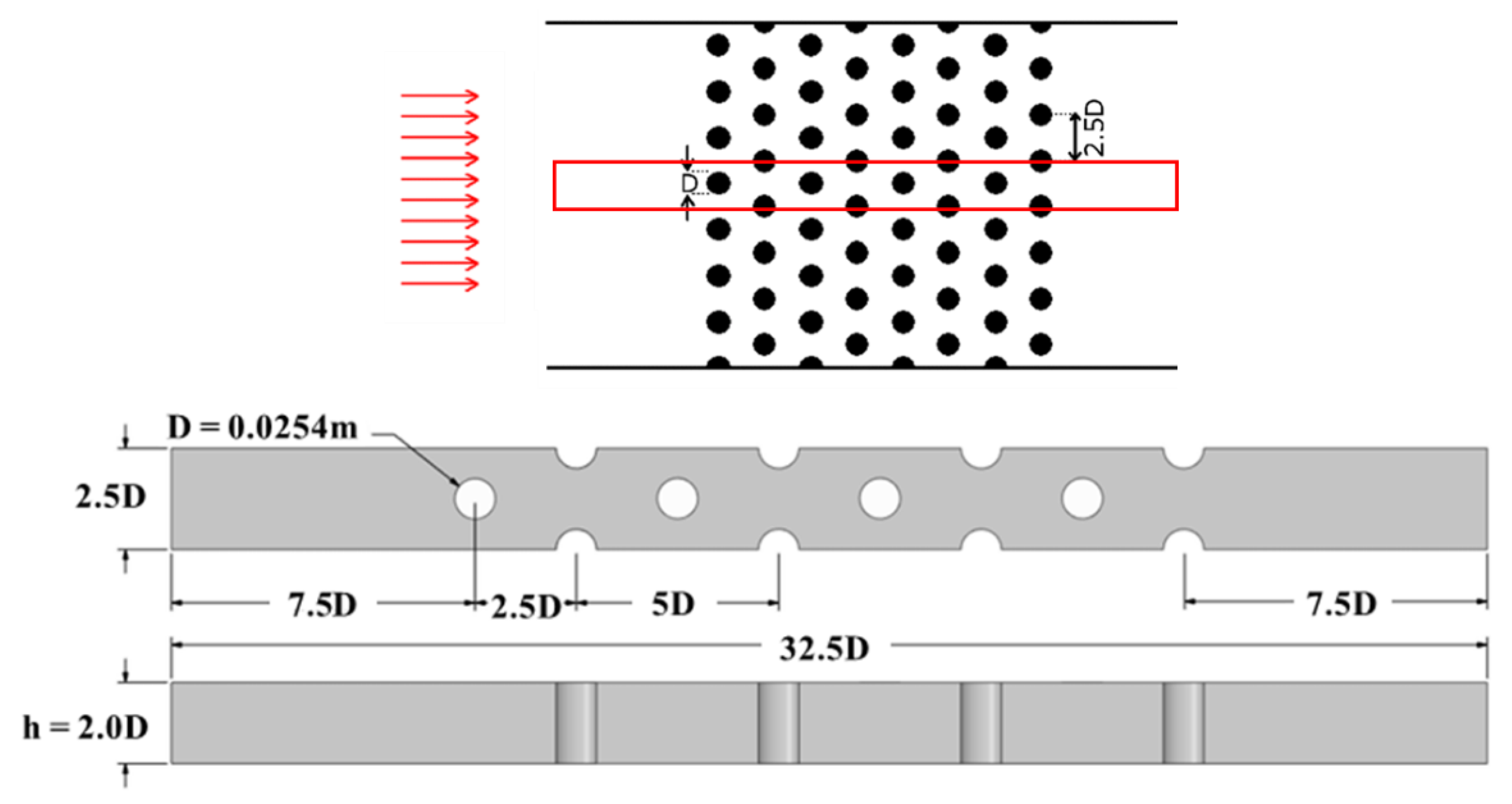
The geometry in the present work is adopted from the experiments of Ames et al. [4,5,6], which consists of multiple pins attached at the plane. The cylindrical pins with diameter D = 0.0254 m are located in a staggered array with a distance of 2.5 D between each pin and each row of pins. The channel height is set to 2 D. For efficient simulation, the periodic segment geometry is considered, which is the same as in simulations by Delibra et al. [7,8,9]. The spanwise length of the channel is 2.5 D and the first row of pins is set to 7.5 D away from the inlet for development of boundary layers on end-walls. The distance between the last row of pins and the outlet is also 7.5 D to retain a fully developed exit flow for better numerical convergence. The total length in the streamwise direction is 32.5 D. Details of the geometry and computational domain are shown in Figure 1.

The numerical analysis is performed by commercial software ANSYS Fluent v. 18.2 [16] to solve unsteady incompressible Navier-Stokes equations and energy equations for convective heat transfers. The SIMPLEC algorithm is used for pressure and velocity coupling. All of the spatial terms are discretized by using the second-order upwind scheme, and the unsteady term is discretized in the second-order implicit method. The time step size, Δt, is set to 0.001 s. In the present work, one URANS model and two hybrid RANS/LES models are considered; the URANS model is the k-ω SST Langtry-Menter transition model, and the two hybrid RANS/LES models are IDDES and SBES models.

The SST transition model is a local correlation-based transition model (LCTM) proposed by Menter et al. [17]. This model solves two other transport equations, one for the intermittency (γ) and one for the transition onset criteria (Re_θ), based on the k-ω SST model. The LCTM approach can predict the transitional point from the transport equation with empirical correlation and show good agreement with experimental data of transitional flow around Aerospatiale A-airfoil, DLR F5 wings and turbine blade. The details of IDDES and SBES models are described in the next chapter.

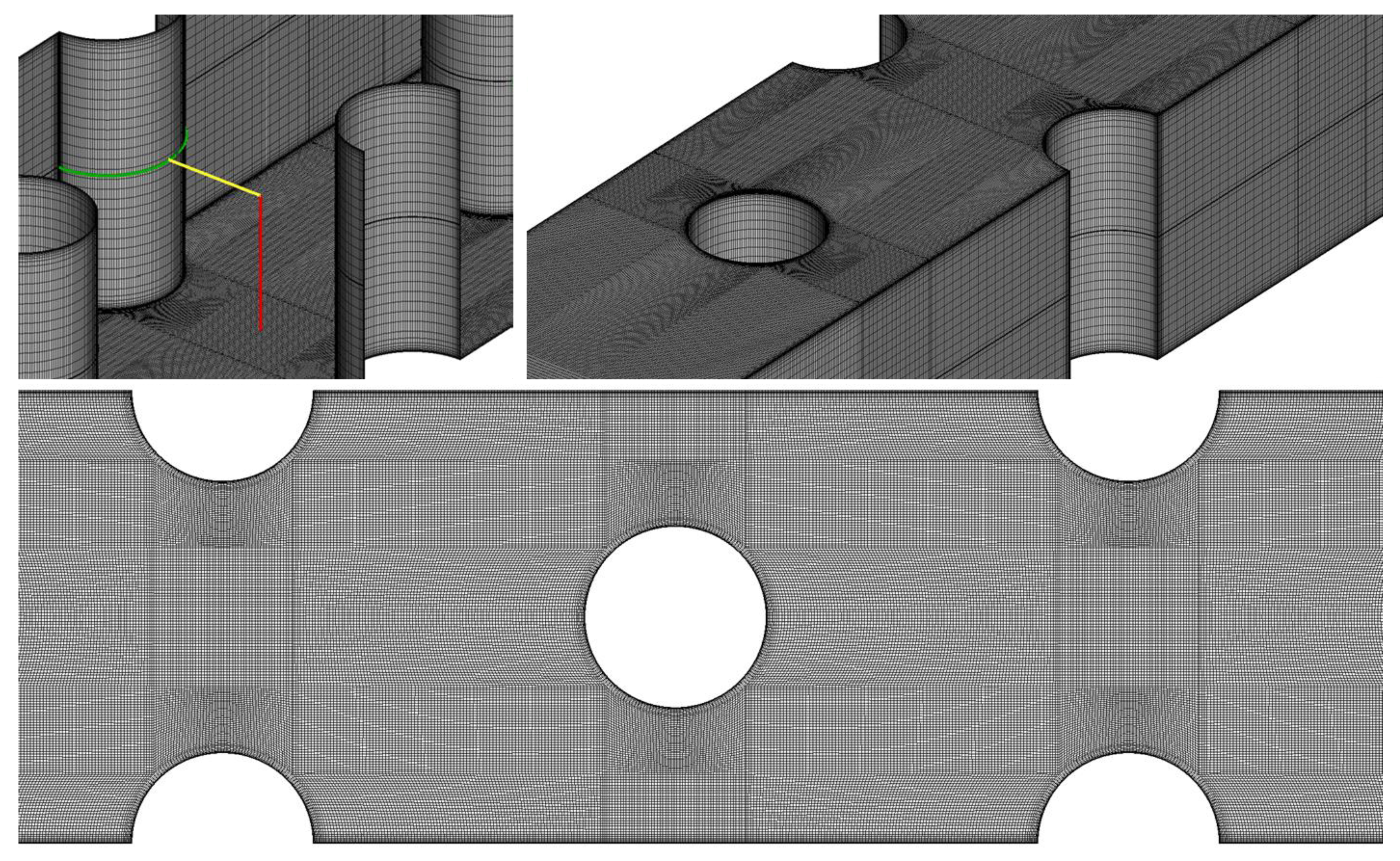
The grid is generated with hexahedral mesh in multi-blocks using ANSYS ICEM CFD [18]. To resolve the turbulent boundary layer near the wall at the bottom and the cylinder pins, 10 layers of mesh are inserted off the wall. The first grid height off the wall is set to satisfy the wall unit within 1.0, which is averaged in the computational domain. The total number of cells corresponds to 14,043,965. The grid system adopted in the present simulation is shown in Figure 2.

The Reynolds number, which is based on the diameter D and the averaged velocity V_max at the minimum passage, is 10,000. The turbulent intensity of the inflow is set to 1.5%, the same as in the experimental conditions of Ames et al. [4,5,6] and the numerical simulations of Hao and Gorle. [10] The hydraulic diameter is set to 0.05664 m. The periodic boundary conditions are applied on both side surfaces, and the pressure outlet conditions are at the outlet. At the end wall and pin wall, the same constant temperature condition is applied as in Delibra et al. [7,8,9]. The temperature difference ΔT (ΔT = T_wall − T_in) between the inlet temperature T_in and the wall temperature T_wall is set to 25 K.

3. IDDES Model Formulation

The IDDES model [19] combines the DDES model [20] and the wall-modelled LES (WMLES) model [21,22]. The original DES model proposed by Spalart et al. [20] is known to be abnormally sensitive to mesh resolution, which determines the length scale between the RANS model and the sub-grid scale model. If the change of grid density is abrupt or if the mesh is not refined enough for a WMLES, the modelled turbulence and eddy viscosity decreases. This phenomenon is called modelled stress depletion (MSD), which causes early unphysical separation termed grid-induced separation (GIS) [20]. The GIS deteriorates the solution near the regions between the RANS mode and the LES mode. Moreover, the DES model shows a relatively strong logarithmic layer mismatch (LLM) between the inner RANS and the outer LES [23]. This issue of LLM is also shown in the DDES model, and the IDDES was proposed to overcome this problem [21]. The IDDES model has a feature to switch the turbulence length scale in the dissipation term of the turbulent kinetic energy equation:

$$\frac{\partial \left(\rho k\right)}{\partial t}+\nabla ·\left(\rho \mathbf{u}k\right)=\nabla ·\left[\left(\mu +{\sigma }_k{\mu }_k\right)\nabla k\right]+P_k-\rho \sqrt{k^3}/l_{IDDES}$$

(1)

$$l_{IDDES}={\tilde{f}}_d·\left(1+f_e\right)·l_{RANS}+\left(1-{\tilde{f}}_d\right)·l_{LES}$$

(2)

$$l_{LES}=C_{IDDES}\Delta , l_{RANS}=\frac{\sqrt{k}}{C_{\mu }\omega }$$

(3)

$$\Delta =\underset{}{\min }\left\{C_{\omega }\underset{}{\max }\left[d_w , h_{max}\right] , h_{max}\right\}$$

(4)

where Δ is the LES length scale and h_max is the maximum edge length of the cell. d_w denotes the distance from the wall.

$${\tilde{f}}_d=max\left\{\left(1-f_{dt}\right), f_b\right\} , f_{dt}=1-\tanh \left[{\left(C_{dt1}·r_{dt}\right)}^{C_{dt2}}\right]$$

(5)

$$r_{dt}=\frac{{\nu }_t}{{\kappa }^2{d}_w{}^2\sqrt{0.5\left(S^2+{\mathsf{\Omega }}^2\right)}} , r_{dl}=\frac{\nu }{{\kappa }^2{d}_w{}^2\sqrt{0.5\left(S^2+{\mathsf{\Omega }}^2\right)}}$$

(6)

$$f_b=min\left\{2exp\left(-9{\alpha }^2\right) , 0\right\} , \alpha =0.25-\frac{d_w}{h_{max}}$$

(7)

$$f_e=f_{e2}·max\left(\left(f_{e1}-1.0\right), 0\right)$$

(8)

$$f_{e1}=\{\begin{array}{c}2exp\left(-11.09·{\alpha }^2\right) when \alpha \ge 0\\ 2exp\left(-9·{\alpha }^2\right) when \alpha <0\end{array} f_{e2}=1-max\left(f_t , f_l\right)$$

(9)

$$f_t=\tanh \left({\left(C_t{}^2·r_{dt}\right)}^3\right) , f_l=\tanh \left({\left(C_l{}^2·r_{dl}\right)}^3\right)$$

(10)

f_dt is the empirical function for shielding of the DDES model from MSD, which is similar to f_d in the DDES model. υ and υ_t are the molecular and eddy viscosity, respectively. S and Ω are the strain rate and vorticity tensor. Detailed formulations and related constants can be found in Gritskevich et al. [19].

4. SBES Model Formulation

An SBES turbulence model was proposed by Menter [13] considering the ability to blend the RANS model directly into LES model based on the same shielding function f_SDES of the SDES model [16] Menter [13] recommended this method, “Automatic Zonal Modeling,” to satisfy

(1)

a high degree asymptotic shielding of the RANS boundary layer under mesh refinement

(2)

reliable and swift switching from RANS to LES in separate shear layers (SSLs)

(3)

operation in WMLES mode

(4)

able to combine all RANS and all LES models

(5)

robustness even on non-perfect industrial meshes.

The equation for the blending of stress tensors can be expressed as:

$${\tau }_{ij}^{SBES}=f_{SDES}{\tau }_{ij}^{RANS}+\left(1-f_{SDES}\right){\tau }_{ij}^{LES}$$

(11)

where ${\tau }_{ij}^{RANS}$ is the RANS Reynolds stress tensor and ${\tau }_{ij}^{LES}$ is the LES stress tensor. In the case of the eddy viscosity model, the formulation above simplifies to

$${\mu }_t^{SBES}=f_{SDES}{\mu }_t^{RANS}+\left(1-f_{SDES}\right){\mu }_t^{LES}$$

(12)

when $f_{SDES}$ is zero, the RANS model is applied; when the $f_{SDES}$ is 1, the algebraic LES model is applied. In the present work, the two-equation model (k-ω SST) is used for the RANS model, and the Wall-Adapting Local Eddy-viscosity (WALE) model is adopted for the LES model. The SBES model can switch from the RANS model to LES faster than the other hybrid RANS/LES models in separate layers since the level of turbulence stress of the LES model in the RANS boundary layer is low. As a result, the solution is more realistic and consistent.

5. Results

The grid test is achieved using coarse (10 million cells), medium (14 million cells), and fine mesh (20 million cells), which is shown in

Table 1. Grid independence test.

$\mathit{N}{\mathit{u}}_{\mathit{a}\mathit{v}\mathit{e}}$	Coarse	Medium	Fine
Number of cells	10,165,687	14,043,965	20,564,381
Maximum y+	1.45	1.32	1.16
Average y+	0.15	0.14	0.14
IDDES	45.11	43.46	41.54
SBES	46.74	44.61	43.47

, based on the adopted hybrid RANS/LES models, IDDES and SBES. To resolve the turbulent boundary layer, the first off-wall point is set to less than the wall unit, 1.0 in all meshes. The maximum and average values of y+ quantity are shown for each mesh. The averaged Nusselt number, which is calculated through averaging from inlet to outlet, is compared for the grid test. In both models the averaged Nusselt number decreases as the number of elements increases, but the result of SBES is closer to the reference value and LESs other than the IDDES model. Further, the differences between the coarse mesh and fine mesh are about 8.2% and 7.2% in the IDDES and SBES model, respectively, which means the dependency of the mesh is higher in IDDES than in SBES. 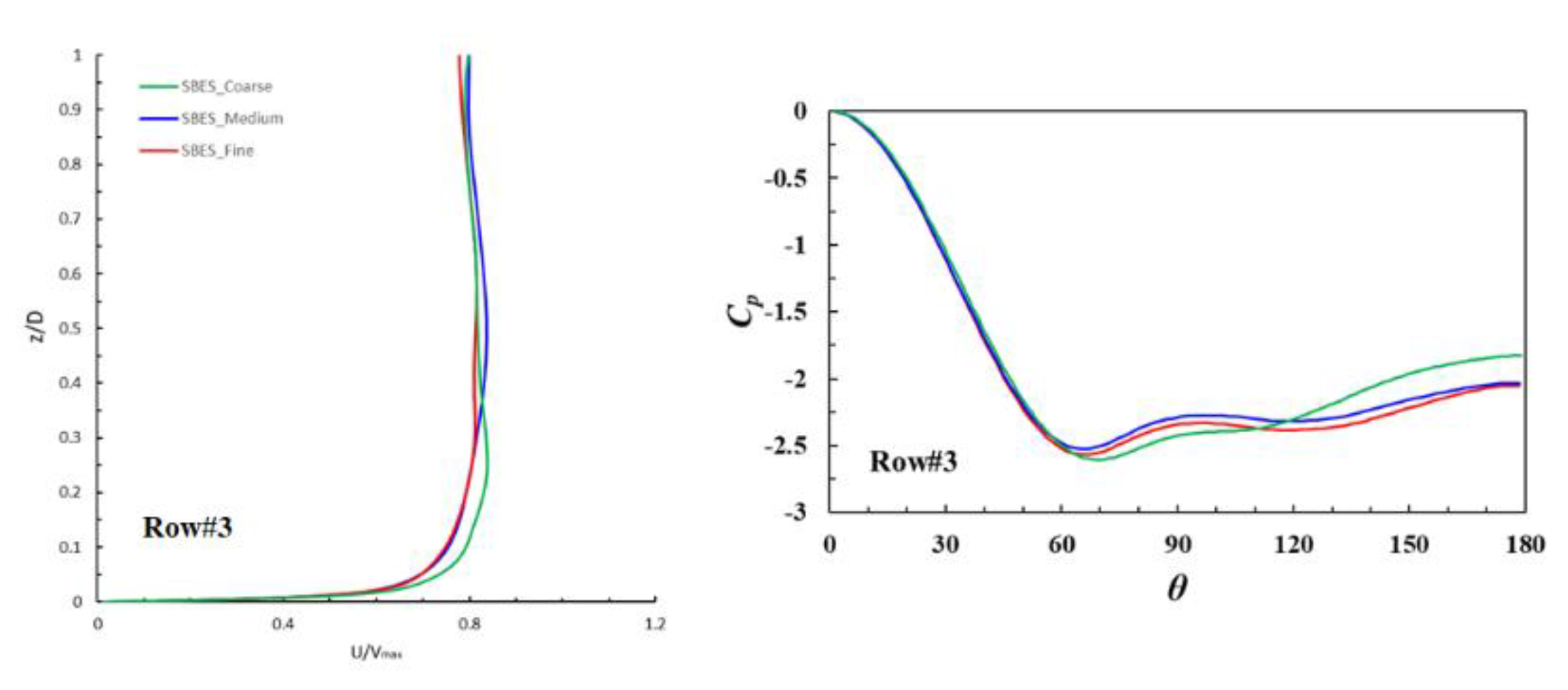Figure 3 shows the mean streamwise velocity and pressure coefficient for row 3 of each grid in the SBES model. There is little difference between the results of medium and fine mesh but the results in coarse mesh show a large discrepancy with the other two cases. Thus, the medium grid with 14 million cells is selected as appropriate given the associated computational time and cost. The total computational time spent to perform each case using 22 cores correspond to 154, 234, and 150 h for k-ω SSTLM, IDDES, and SBES, respectively.

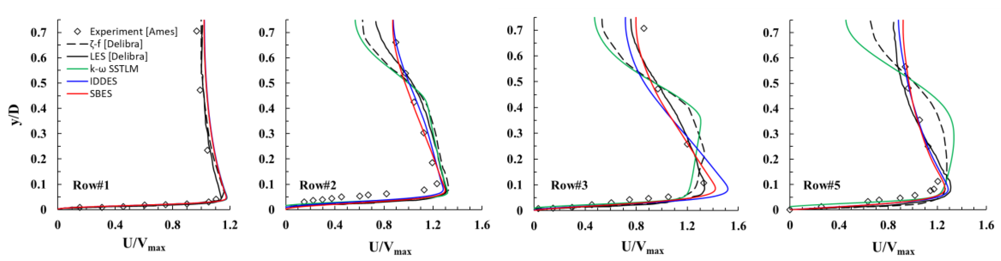
Figure 4 shows the mean velocity profiles normalized by V_max along the line between a certain row of pins (at 90°) at the middle height plane (z/D = 1.0). The velocity profiles are averaged in enough time (~6000-time steps) to obtain statistically steady solutions in every model. The experimental data by Ames et al. [4,5,6] are denoted by the diamond symbol; the two CFD results by Delibra et al. [7,8,9] are the LES data (solid black line) and the URANS data (black dashed line) for comparison with the present results. The other three lines (green, blue, and red) correspond to the present results: k-ω SSTLM, IDDES, and SBES, respectively. In the first row, all of the simulation results are good agreement with the experimental data. In the other rows, the two hybrid RANS/LES models agree well with the LES results (row 5) and the experimental data (rows 1, 2, and 3), but the ζ-f URANS [8] and k-ω SSTLM models predict different velocity profiles with large discrepancies, especially near the center between the pins.

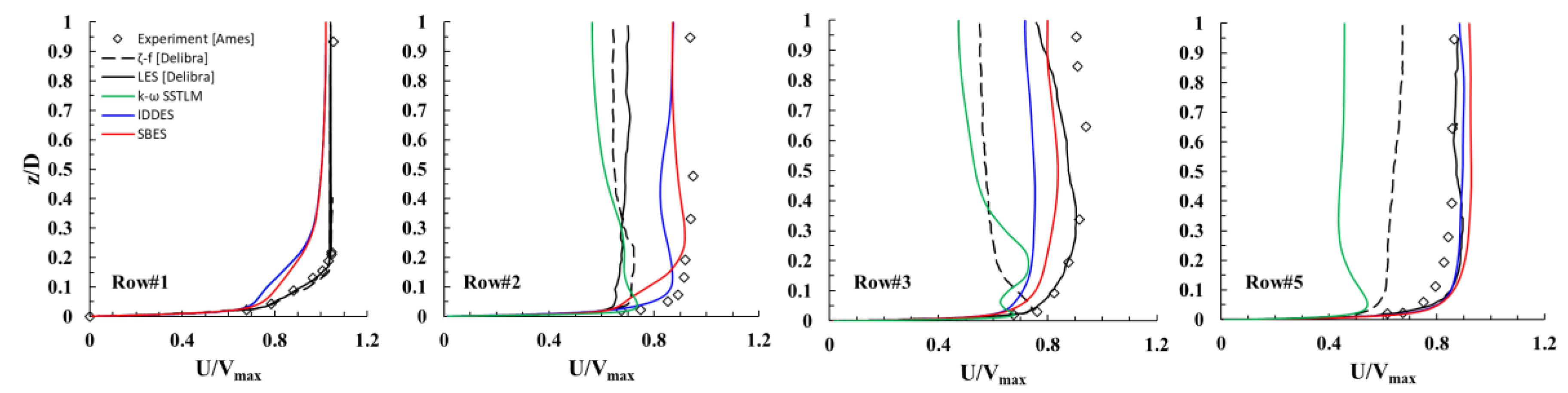
The mean velocity profiles along the perpendicular line on the end-wall are plotted in Figure 5. The turbulent boundary layer profile, which was obtained from other simulations in the corresponding channel geometry with up-and-down walls, was fed at the inlet of the computational domain, the three present results show discrepancies with other reference data in the first row. However, the boundary layer of the two hybrid RANS/LES models was developed appropriately and follows the tendency of the experimental data. In the second row, IDDES and SBES show magnitudes of velocity similar to the experimental data, but the URANS and LES models show less velocity. In the third row, the SBES result is closer to the LES results and the experiment data than are the IDDES and other URANS models. Finally, the velocity profiles of IDDES and SBES agree well with the LES profile. In every row, the two URANS models produced large discrepancies with the reference data.

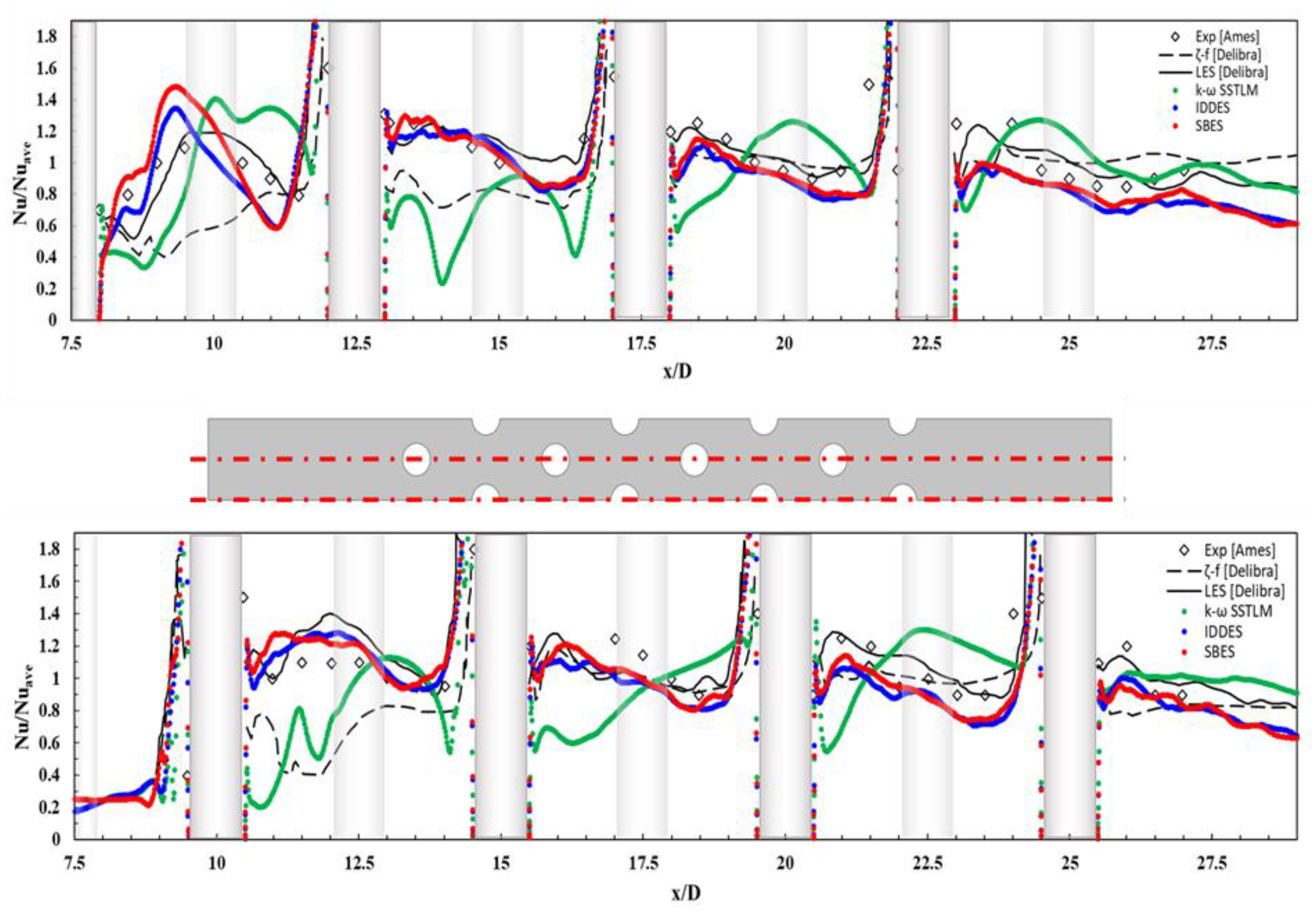
Figure 6 shows the local Nusselt numbers normalized by averaged Nusselt numbers along the middle line (A) and the side line (B) on the end-wall. For clear recognition of the calculated local Nusselt numbers, the results of the present work are plotted in the same colors as in the other figures. In previous research, most of the URANS models failed to predict the local Nusselt number distributions similarly with experimental results (rows 1, 2, and 3), whereas some LES models were able to follow the shape of the distribution of the local Nusselt numbers (row 5). The two hybrid RANS/LES results show superior prediction similar to the previous LES results and experiment data. The Nusselt number shows an abrupt increase near the upstream wall of each pin and a gradual decrease after the downstream wall of a pin. IDDES and SBES were able to predict these behaviors well and agreed well with the LES results. However, the values predicted by the two hybrid RANS/LES models are underestimated compared to the reference values as the flow goes downstream. This underestimation comes from the lack of resolving the vortex shedding after the pins. On the other hand, the LES model resolves enough vortex structures by having enough mesh and inherent model characteristics.

The k-ω SSTLM model is not able to follow the variation of local Nusselt numbers in most of the regions, which is consistent with the results of k-ω SSTLM modeling by Carnevale et al. [11] Benhamadouche et al. [24] investigated the assessment of three URANS models (EB-RSM, k-ω SST, and ϕ-model) and an LES model in the present geometry, and determined that the k-ω SST and the ϕ-model (a stabilized version of the v²-f model) underestimated Nusselt numbers after the first few pins where the turbulence was not yet fully developed and mixing was dominant. As the k-ω SSTLM model is a transitional model rather than a fully developed turbulent one, its prediction of Nusselt numbers after the first pin is slightly better than the other two fully developed turbulent models investigated by Benhamadouche et al. [24] However, there are still large discrepancies in the other pins, which show behavior similar to the results of the ϕ-model [24].

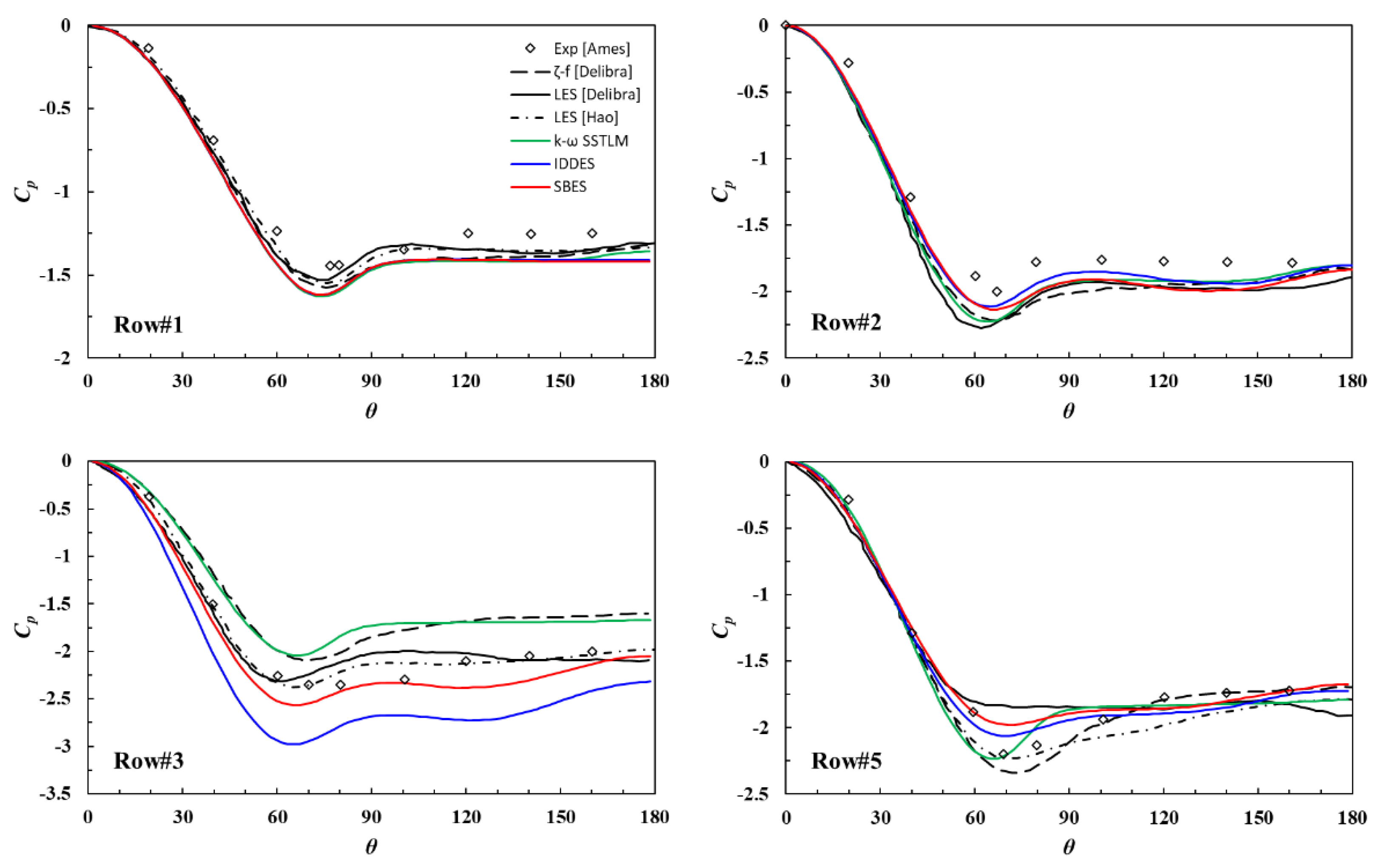
The averaged pressure coefficients around the pins for rows 1, 2, 3, and 5 are plotted in Figure 7. The pressure coefficient distribution is calculated following the below definition, Equation (13):

$$C_p=\frac{2\left(p-p_0\right)}{\rho V_{max}^2}$$

(13)

where $p_0$ is the mean pressure at the leading edge. Every model shows consistent predictions of the pressure coefficient at the first and second row, but there are some discrepancies in the other two rows. At the third row, the difference between each model is largest and the predictions of the two LES models by Delibra et al. [7] and Hao and Gorle [10] are closest to the experimental data. In the present work, the SBES model shows predictions closest to the reference data, and the two LES models and the k-ω SSTLM model have patterns similar to the ζ-f model by Delibra et al. [8] At the fifth row, even though each model shows a similar prediction in the region of the attached flow and after the separation point, there is a large discrepancy between θ = 50° and 100° in the prediction of each model. Delibra et al. [8] showed that the ζ-f model’s pressure coefficient prediction at the fifth row was better than the LES model’s, which is shown in Figure 7. They mentioned that this was not in conflict with the excellent LES predictions of the mean velocity in the cross-section as this agreement did not guarantee the accurate prediction in the pin wakes. The LES model by Hao and Gorle [10] best predicted this coefficient in the fifth row, even though that model had a slower pressure recovery (with a maximum difference of 13%) among all the models considered in the present work. The predictions of the two hybrid RANS/LES models in the present work are between the results of the two LES models.

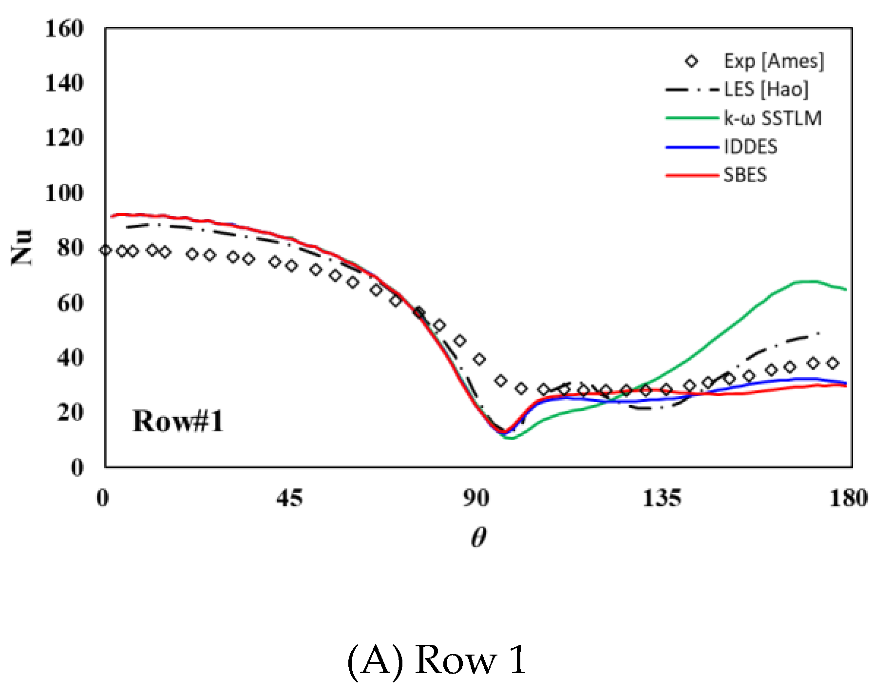
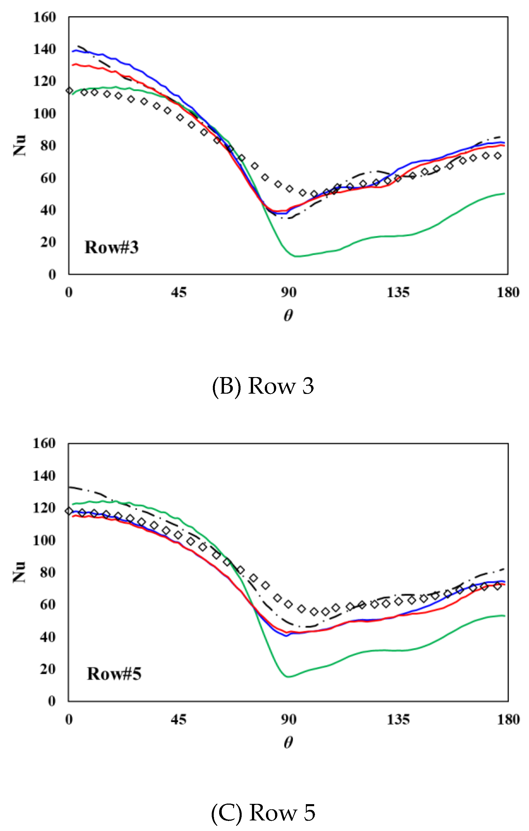
Figure 8 shows the distributions of the Nusselt numbers around the pins for rows 1, 3, and 5. The Nusselt number is calculated using the expression

$$Nu=qD/k_{air}\left(T_b-T_{in}\right)$$

(14)

where $q$ and k_air are the wall normal heat flux and thermal conductivity, respectively, and $T_b$ is the bulk-flow temperature. The Nusselt number distribution shows the highest value at the leading edge of each pin, and decreases along the pin surface; after separation the value plateaus or increases gradually. The results of IDDES and SBES agree well with the experimental data and the LES results of Hao and Gorle [10] in the whole region. The IDDES and SBES models overestimate the Nusselt number at the leading edge, the same as with the LES model. The difference from the experimental data is about 10% in row 1 and about 10% and 15% for SBES and IDDES, respectively, in row 3. All the numerical models fail to predict the minimum Nusselt number just upstream of the separation points. Hao and Gorle explain that this difference is due to a non-uniformity of the pin surface temperature in the experiment (rows 1, 2, and 3). However, there is a somewhat large discrepancy in the prediction of the k-ω SSTLM model, especially in the region after the separation.

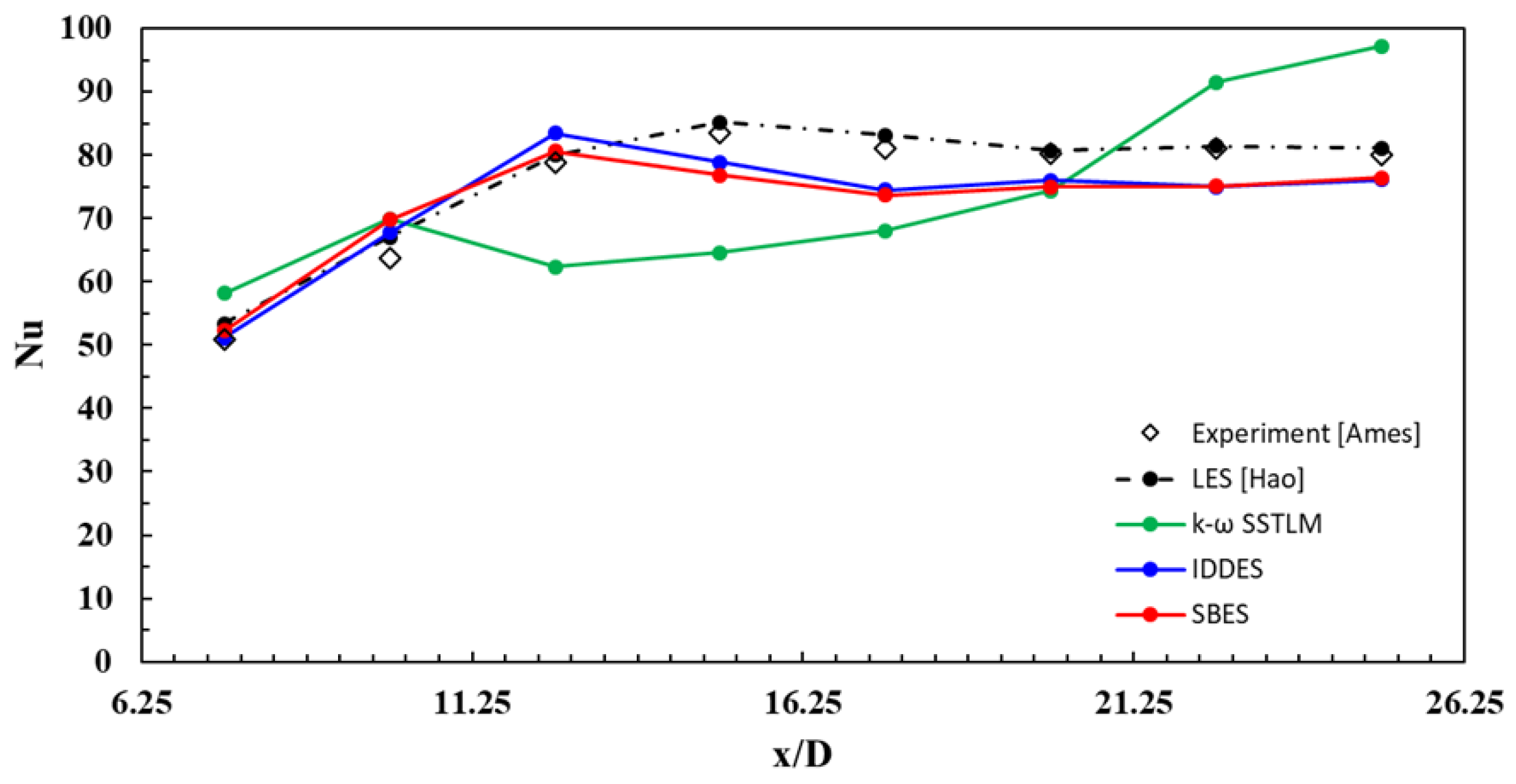
In Figure 9, the predicted Nusselt number around each pin is averaged over the surface and plotted for a total of eight pins. Experimental data and LES results by Hao and Gorle [10] are presented for comparison with the present results. The averaged Nusselt number for each pin increases until the fourth row and then stays constant after a small decrease. The results of IDDES and SBES are fairly consistent with each other and agree well with other reference data until the third row. The predicted Nusselt number decreases after the third row and then stays constant with a maximum difference of 9% from the experimental data. There is still a large discrepancy in the k-ω SSTLM model even though the unsteady temperature and velocity field are averaged in time over enough time. This discrepancy comes from the failure of the correct thermal boundary layer on the pin surface wall.

Table 2. Surface average Nusselt number.

	k-ω SSTLM	IDDES	SBES
$N{u}_{ave}$	41.29	43.46	44.61

summarizes the averaged end-wall Nusselt numbers of the considered models and the reference data. The predicted Nusselt numbers on the end-wall are 44.61, 43.46, and 41.29 by SBES, IDDES, and k-ω SSTLM, respectively. Even though these values are about 20% discrepant from the experimental data [6], they are similar to the values predicted by other numerical simulations, LES [7] and hybrid RANS/LES. Delibra et al. [7,8,9] mentioned that deviations between experimental data and numerical simulation are caused by heat escape by radiation and/or heat sink in the experiment. Although numerical simulations do not consider this effect, an LES model with about 11 million mesh cells by Hao and Gorle [10] predicted the averaged end-wall Nusselt number as 53.5, within 1% of the experimental data result.

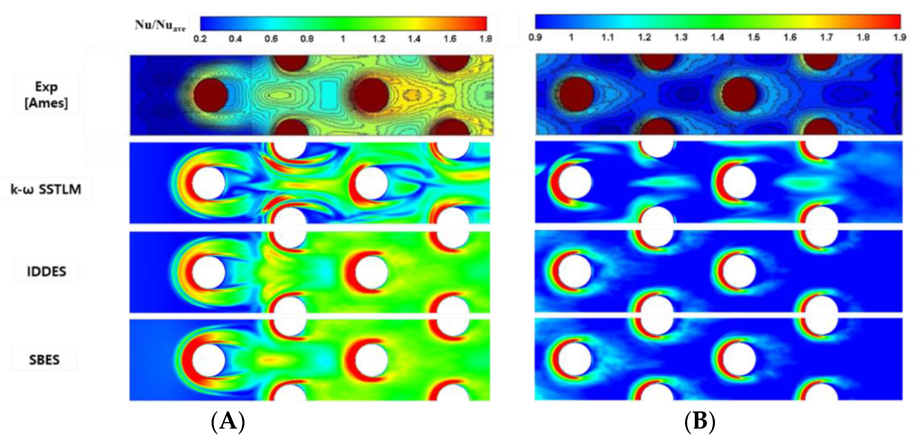
Figure 10 shows contours of Nusselt numbers normalized by averaged Nusselt numbers on the end-wall in the upstream region (A) and downstream region (B) of the experimental data and the present results. The upstream min, max = 0.2, 1.8, and the downstream min, max = 0.9, 1.9 of the Nusselt numbers in all the models are the same as in the experimental data presented by Ames [6]. The Nusselt number is relatively low near the inlet and high in the region of the leading edge.

The SBES results show the best agreement with the experimental data, in particular the high Nusselt number in the passage between the second row, and the pattern of this number distribution in the wake region after the fifth and seventh rows. The IDDES model can predict a similar distribution overall but there are small differences in the regions as mentioned above. The k-ω SSTLM model shows different patterns in the high-velocity passage between two symmetric rows, and the contours do not look symmetric even with enough time-averaging. Benhamadouche et al. [24] suspected the presence of very low frequencies that are not physical during solving the governing equations pertaining to non-symmetric flow patterns in the k-ω SST model. In the IDDES and k-ω SSTLM models, the Nusselt number near the leading edge of the first-row increases, then slightly decreases, and then increases again, whereas the SBES model shows a gradual increase without any decreases. This can be confirmed by the local Nusselt number distributions in Figure 6. This abnormal behavior is related to the prediction of horseshoe vortex structures near the leading edge of obstacles attached to the wall.

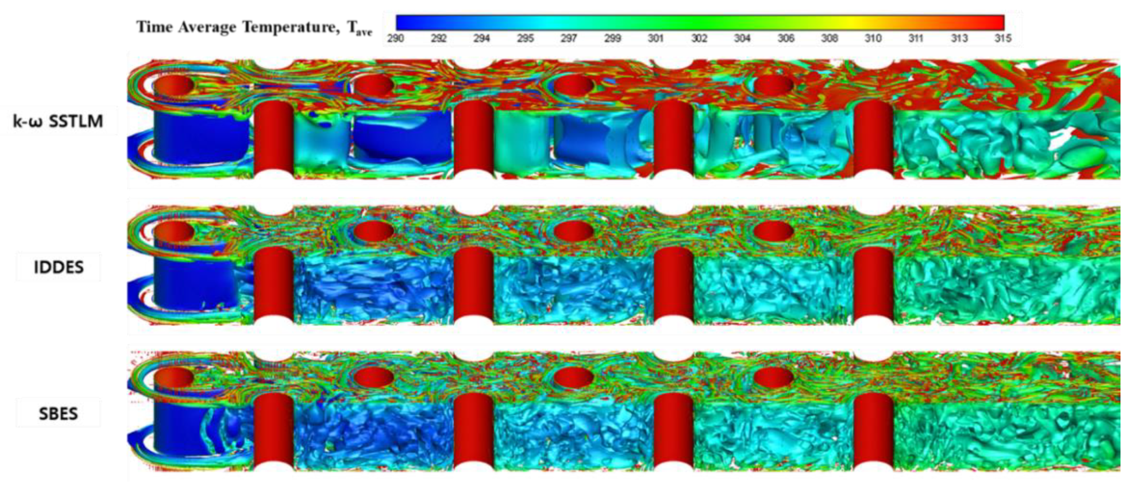
The vortical structures of instantaneous flow fields are investigated with a Q-criteria value of 10 [25] in Figure 11. These iso-surfaces are colored by temperatures from 290 K to 315 K, and the flow field is heated gradually as the flow moves downstream. Horseshoe vortices, which are also shown in Figure 12, can be recognized in front of the pins but it is difficult to identify them in the downstream pins. A vortex tube in the spanwise direction from each pin is generated after separation from the first pin and breaks down into 3-D vortices in the streamwise direction interacting with downstream pins. The two hybrid RANS/LES models, IDDES and SBES, are better able to resolve smaller vortex structures than the k-ω SSTLM model, as shown in Figure 11, and they show similar structures when compared with other LES results [7,10]. In the k-ω SSTLM model, 2-D vortices are sustained until the sixth pin and then break into 3-D flow features that are larger than in the other models. Of particular note is that SBES can capture the distorted spanwise vortex tube after separation from the first pin, whereas the IDDES and k-ω SSTLM models fail to predict it even with the same grid numbers and Q-criteria value.

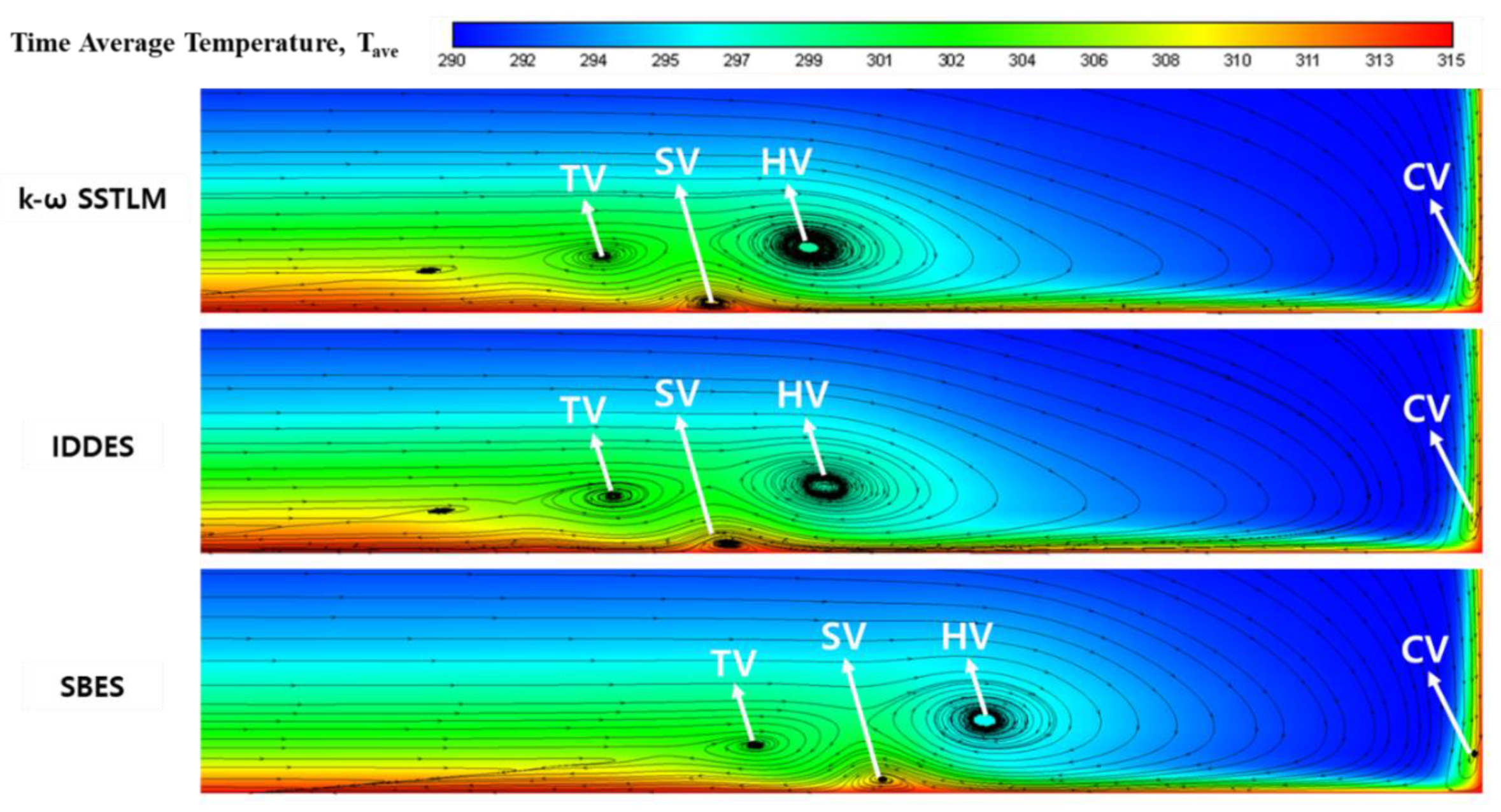
Figure 12 shows time-averaged streamline patterns and temperature contours in the front cylinder part at the mid-line of the xz-plane. As mentioned above, the three models can capture the horseshoe vortex system, including HV (horseshoe vortex), SV (secondary vortex), and TV (tertiary vortex). The SBES model predicts this vortex system slightly closer to the first cylinder wall than the other two models do, and the CV (corner vortex) is shown clearly in the SBES model. Interestingly, the region where the horseshoe vortex systems are predicted is coincident with the region where the LES mode is active in the SBES model.

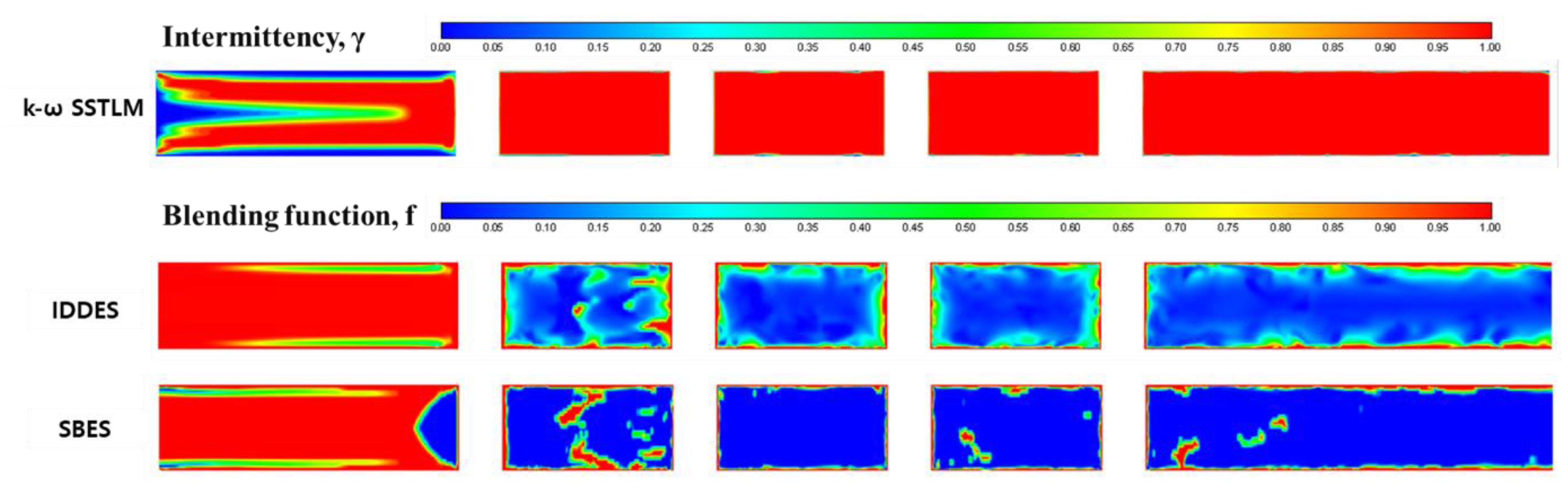
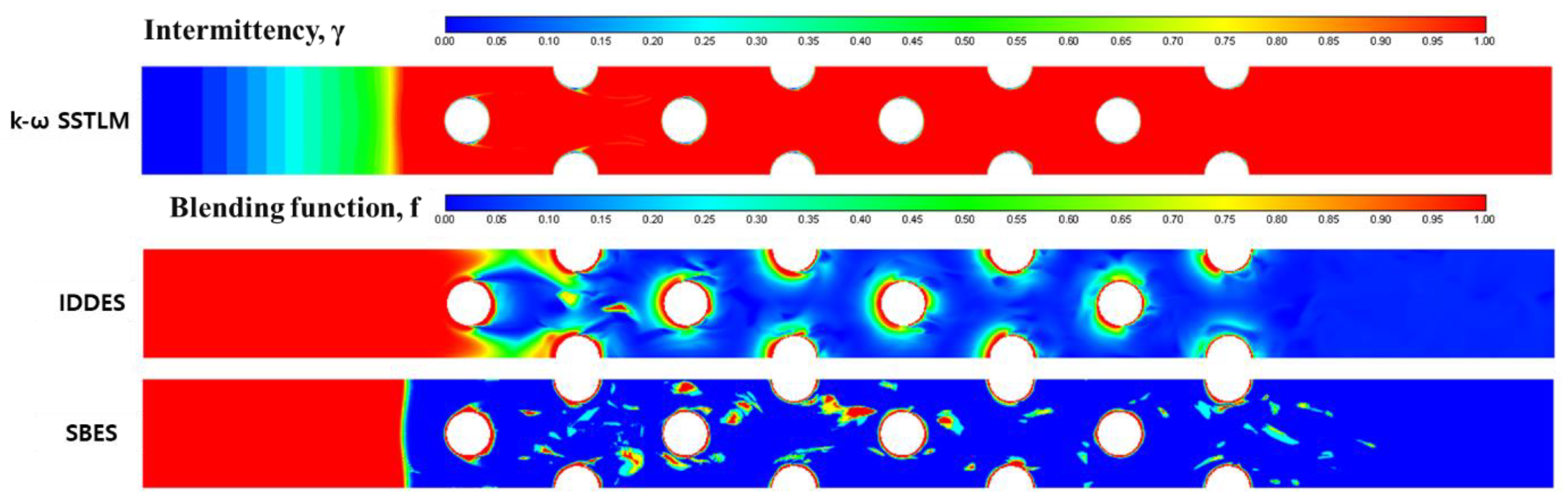
To investigate the effects of the blending function which changes the turbulence model between RANS and LES, the contours of the blending function are plotted in Figure 13 and Figure 14 with respect to two planes: the xz-plane at the mid-line of the y-axis and the xy-plane at the center height of the z-axis. The value 1 means the RANS method is adopted and 0 is for the LES method. Since the k-ω SSTLM model is not a hybrid RANS/LES method but, rather, a transitional model, the intermittency (γ) which reflects laminar flow with a 0 value and turbulent flow with 1 is contoured at the same planes. As can be seen in the two figures, the SBES model adopts the LES calculation in a larger region than that of the IDDES model, and shows a sharp transition from RANS to LES; in contrast, the IDDES model changes the two methodologies smoothly. In front of the first pin, the LES calculation is changed more rapidly in the SBES model than in IDDES. This is why the results of the SBES model more closely resemble LES results than do the other models.

However, non-uniformity of the blending function can be found in the SBES model even with long-time averaging of the flow field. In the k-ω SSTLM model, as expected, flows near the inlet are predicted in laminar flow and then develop into the turbulent flow which is sustained until the outlet of the computational domain. Menter [13] mentioned that the shielding function in SBES can cover the boundary layer, including the rapid growth area by the adverse pressure gradient, while the shielding function of DDES impairs this region. In the computation domain of the present work, a total of 12 cylinders (4 cylinders at the mid-line and 8 half-cylinders at the periodic plane) experience adverse pressure gradients in the back part (approximately θ > 90°) of each cylinder. As seen in Figure 13 and Figure 14, the SBES model implies a clear and sharp RANS mode near the cylinder walls, but the IDDES model does not show a continuous and smooth transition between RANS mode and LES mode near the wall.

6. Conclusions

In the present work, two hybrid RANS/LES modes, IDDES and SBES, and one transitional URANS model, k-ω SSTLM, are adopted to investigate their ability to predict heat and fluid flow phenomena around staggered pin-fin arrays. The corresponding Reynolds number based on the pin diameter and the maximum velocity between the pins is 10,000, and the periodic segment geometry with a total of eight pins is considered. The simulated results, including mean velocity, pressure, local and global Nusselt numbers, and coherent structures, are compared with experimental data [4,5,6] and other LES [7] and URANS [8] results.

Mean velocity profiles predicted by IDDES and SBES agree well with the reference data, but the k-ω SSTLM model shows large discrepancies near the centers between the pins. In averaged pressure coefficients around the pins, the SBES model gives the closest prediction in the region of the attached flow and after the separation point, compared to all the other models in the present work. The results of the k-ω SSTLM model are similar to those of the other URANS model, the ζ-f model [8], with large discrepancies in the separated region.

The two hybrid RANS/LES models show superior predictions of the nonlinear behavior of local Nusselt numbers, with abrupt increases near the upstream of each pin and gradual decreases after the downstream wall. However, in the region downstream of the pins they slightly underestimate the local Nusselt number because they do not resolve the vortex shedding after the pins fully. In the k-ω SSTLM model, the transitional behavior around the first pin is predicted well but there are large discrepancies around the other pins, the same as with the other URANS model. Similarly, the two hybrid RANS/LES models predict the distributions of Nusselt numbers around the pins and the averaged Nusselt number in each section of pins, very similar to the other LES results.

Vortical structures, including horseshoe vortex systems in front of the first pin and wakes after each pin, are fully resolved in the two hybrid RANS/LES models, very similar to the LES model. In particular, the SBES model can capture the distorted spanwise vortex tube after separation from the first fin, whereas IDDES and k-ω SSTLM fail based on the same grid system.

In our investigation of the effects of the blending function of the two hybrid RANS/LES models, the SBES model adopts the LES calculation in a larger region with a sharp transition from RANS to LES, compared to the IDDES model. Therefore, the SBES prediction more closely resembles the LES results.