Stochastic NPV Based vs Stochastic LCOE Based Power Portfolio Selection Under Uncertainty

Abstract

This paper investigates the problem of power portfolio selection under uncertainty using two different metrics, namely the stochastic Net Present Value (NPV) and the stochastic Levelized Cost of Electricity (LCOE). In the first metric, stochastic revenues, as well as stochastic costs incurred during the whole lifetime of power plants, are taken into account. The second metric is based on stochastic costs only. This means that revenues deriving from selling electricity in power markets over long-term horizons play an important role in determining optimal portfolios under the stochastic NPV metric, but they have no impact on optimal portfolios under the stochastic LCOE metric. Uncertainty arising from unpredictable movements of electricity market prices, fossil fuels, and nuclear fuel prices is considered. Moreover, stochastic CO${}_2$ costs are included into the analysis. The aim of this study was to examine in what circumstances efficient NPV-based portfolios differ in a significant way from efficient LCOE-based portfolios. The portfolio selection is performed using two different risk measures, namely the standard deviation and the Conditional Value at Risk Deviation (CVaR) deviation. The proposed methodology can be used as a powerful tool of analysis for planning profitable investments in new generating technologies paying attention to risk reducing strategies through power sources diversification.

1. Introduction

Risk reducing strategies through diversification of power generating assets can be a very important solution for electricity companies in their attempts to hedge financial risk arising from unpredictable movements of electricity market prices, fossil fuels, and nuclear fuel prices [1]. Moreover, environmental policies based on the reduction of CO${}_2$ emissions through market pricing mechanisms [2,3] require also taking into account the impact on generation costs of volatile CO${}_2$ prices [4,5]. All these factors are, in fact, the main sources of financial risk in the electricity sector [6].

This paper addresses the power portfolio selection problem under uncertainty for baseload generation. Two cases are discussed, namely the case of a pure fossil fuel (gas and coal) generation company and the case of a pure baseload company with fossil fuel and nuclear power generating assets. Many companies now break up their previous diversified generation portfolios to create new companies that are, e.g., pure fossil, on the one hand, and pure nuclear, on the other. From this point of view, the problem of finding optimal generation mixes is a relevant task not only for the new companies but also for the holding company that owns other companies’ outstanding stock.

The analysis is performed at two different levels, namely at a cost-benefit level, using as evaluation metric the stochastic Net Present Value (NPV), and at a cost level, basing the analysis on the stochastic Levelized Cost of Electricity (LCOE) metric [7]. In the first metric, stochastic revenues, as well as stochastic costs incurred during the whole lifetime of power plants, are taken into account. The second metric is based on stochastic costs only. Revenues deriving from selling electricity in power markets over long term horizons play, therefore, an important role in determining optimal portfolios under the NPV stochastic metric. On the other side, revenues are not included in the stochastic LCOE metric and, in such a case, the portfolio selection is based on stochastic costs only. The aim of this paper was to investigate the composition of optimal portfolios under the two different metrics.

For each metric, the power portfolio selection is performed under two different risk measures, namely the standard deviation and the Conditional Value at Risk Deviation (CVaRD) [8,9]. The standard deviation is used to describe the risk due to fluctuations around the mean of the stochastic metric used; the CVaRD is used to capture the tail risk due to extreme adverse events. Power source diversification, in fact, offers the possibility to investigate the trade-off between risk, as measured by the standard deviation or by CVaRD of the stochastic metric used and its expected value. The main purpose of this paper was to derive the composition of the so-called ‘efficient portfolios’ (in a sense that will be specified in the following section) under both stochastic metrics and both risk measures. The aim was to compare the set of efficient portfolios obtained in the stochastic NPV-based portfolio selection problem with the set of efficient portfolios derived in the stochastic LCOE-based portfolio selection problem, as well as to investigate under what circumstances these sets may differ in a significant way.

The main findings are briefly summarized. Since revenues for baseload generation do not depend on the power portfolio composition, efficient portfolio frontiers are invariant with respect to the stochastic metric adopted if the standard deviation is assumed as risk measure. The reason is that annual revenues become stochastically independent from annual costs when they are computed averaging over one year of observations [10]. Although fuel prices and power prices could show some cointegration relationship [11], nevertheless, the correlation between annual revenues and costs may be negligible, especially in diversified power portfolios. This fact is particularly true when electricity prices experience a very erratic dynamics with jump and spikes with a strong mean-reverting behavior, as in actual power markets [12]. The portfolio selection problem can be performed, therefore, using the stochastic LCOE metrics, as well as the stochastic NPV metric, thus providing the same solution. Minimum risk portfolios, as well as efficient portfolios, do not depend on the metric (stochastic NPV or LCOE) adopted. A NPV efficient portfolio is also a LCOE efficient portfolio, and vice versa. Such a result does not hold if the CVaRD risk measure is used. However, if the volatility of annual revenues is not too high (as in this analysis), the efficient frontier invariance is a very good approximation. The LCOE-based portfolio analysis thus provides almost the same results of the NPV-based analysis. The inclusion of stochastic CO${}_2$ costs does not modify this picture under the hypothesis that CO${}_2$ costs have no impact on electricity market prices. In such a case, standard deviation efficient frontiers are invariant with respect to the used evaluation metric, and CVaRD efficient frontiers are almost invariant. The efficient frontiers invariance is broken under a non-zero correlation between revenues and costs. In such a case, efficient frontiers are no more invariant not only under the CVaRD risk measure but also under the standard deviation risk measure. However, if such a correlation is low on the long-run, frontier invariance is a good approximation. As a further result, not all efficient portfolios show positive expected NPVs. From this point of view, the proposed approach can be used as a powerful tool of analysis to select profitable efficient power portfolios, thus providing a quantitative support to electricity companies in their efforts to plan investments in power portfolios paying attention to the trade-off between profitability and risk. In this sense, the proposed methodology allows electricity companies to design optimal power generating portfolios.

The paper is organized as follows. After this introduction, Section 2 discusses the methodological aspects of the paper. In Section 3, the stochastic metrics used in the portfolio selection problem are presented. Section 4 illustrates the dynamic model used to compute revenues and costs of power generation. Section 5 describes the power portfolio selection problem. Section 6 concludes.

2. Methods

When the stochastic NPV is used to investigate the power portfolio selection problem, stochastic revenues deriving from selling electricity in the power market, as well as costs incurred during the whole lifetime of power plants, must be taken into account in a single metric. In general, such costs include construction costs, operations and maintenance costs (O&M), fuel costs, decommissioning costs, and, possibly, CO${}_2$ emission costs, in the case of fossil fuel generation. Several sources of uncertainty must be, therefore, considered. First of all, electricity market prices. Such a source of risk influences revenues. The followed approach is based on modeling revenues on the long-run, starting from analyzing the short-term behavior of electricity market prices. Due to a strong mean-reverting behavior of electricity prices observed in power markets [13], short-term probability distributions of power prices tend rapidly to well-defined stationary distributions [10]. Such stationary distributions will be used to compute revenues over long-term horizons. From the cost side, fossil fuel market prices and nuclear fuel market prices will be considered as the main source of uncertainty. Natural gas prices too show a mean-reverting behavior with stochastic volatility [14]. Stationary distributions coming from short-term mean-reverting jump-diffusion models of natural gas prices are used to compute gas costs over long-term horizons. The dynamics of both coal and nuclear fuel prices does not show a significant mean-reverting behavior [10], and it is described by a Geometric Brownian Motion (GBM). Regarding the nuclear source, the financial risk due to the social acceptance of this technology is not considered in this paper. The reason is that the power portfolio selection problem is performed under the hypothesis that the nuclear power generation is a well accepted technology. Finally, CO${}_2$ stochastic costs are included in the analysis as a further source of uncertainty. CO${}_2$ stochastic prices are assumed to evolve in time, according to a GBM.

In modeling long-term behavior of electricity and fuel prices, macroeconomic views about long-run evolution of these factors must be taken into account [15]. The proposed dynamic model is able to integrate in a satisfactory way the short-term dynamics with macroeconomic long-run forecasts. Although the portfolio selection problem is well treated in the literature [1,14,16] also in the presence of variable renewable energy [17,18], the portfolio selection problem with such an accurate modeling of electricity and fuel prices dynamics has not yet been developed (see DeLlano-Paz et al. [19] for a detailed review).

The main purpose of this paper was to derive the composition of the efficient portfolios under both stochastic metrics and both risk measures. A power portfolio is said efficient if it belongs to the so-called ‘efficient portfolio frontier’. In the case of the stochastic NPV metric, the efficient portfolio frontier (or, simply, the efficient frontier) is defined as the locus of portfolios with maximum expected NPV among all portfolios with same risk level. In the case of the stochastic LCOE metric, the efficient portfolio frontier is defined as the locus of portfolios with minimum expected LCOE, among all portfolios with same level of risk. The aim is to compare efficient portfolio frontiers obtained in the stochastic NPV-based portfolio selection problem with efficient portfolio frontiers derived in the stochastic LCOE-based portfolio selection problem, and to investigate under what circumstances they may differ in a significant way.

The main data source was the ‘Annual Energy Outlook 2019’ [20]. In particular, cost data of power generating technologies were taken from ‘Capital Cost Estimates for Utility Scale Electricity Generating Plants’ [21] and ‘Cost and Performance Characteristics of New Generating Technologies, Annual Energy Outlook 2019—January 2019’ [22], both provided by the U.S. Energy Information Administration. The dynamic model used to describe the evolution of electricity market prices, fossil fuels, and nuclear fuel prices is taken from Lucheroni and Mari [10].

3. The Stochastic NPV of Power Portolios and the Stochastic LCOE

The stochastic Net Present Value (NPV) and the stochastic Levelized Cost Of Electricity (LCOE) are mathematical constructs that allows to introduce risk in the investment valuation process [1,14]. In this section, the stochastic NPV and the stochastic LCOE analysis of power portfolios is developed in a general stochastic framework with k sources of risk. In such a framework, the stochastic path is denoted by $\xi$.

By definition, the stochastic NPV of a given generating technology z is a random variable determined for each path, $\xi$, by the difference between the present value of revenues and the present values of costs incurred during the lifetime of the plant including pre-operations construction costs. It will be denoted by $NP{V}^z\left(\xi \right)$. The stochastic LCOE of the technology z is defined path by path (i.e., for each $\xi$), as that nonnegative real price of the electricity produced by the specific generation technology z, assumed constant over time, that makes $NP{V}^z\left(\xi \right)$ equal to zero. It will be denoted by $P^{\mathrm{LC},z}\left(\xi \right)$. Between $NP{V}^z\left(\xi \right)$ and $P^{\mathrm{LC},z}\left(\xi \right)$, there exists a very useful relationship [10], namely

$$NP{V}^z\left(\xi \right)=(1-T_c)Q^z\sum _{n=1}^M\left[P_n^z\left(\xi \right)-P^{\mathrm{LC},z}\left(\xi \right){(1+i)}^{n-n_b}\right]F_{0,n},$$

(1)

where $T_c$ is the corporate tax rate, and $Q^z$ is the amount of electricity produced by the technology z in one year. $Q^z$, is assumed to be constant over time and can be obtained multiplying the nameplate power capacity of the plant, $W^z$, by the capacity factor of that plant, $C{F}^z$, and by the number of hours in one year (8760), i.e.,

$$Q^z=8760\times C{F}^z\times W^z,$$

(2)

and $P_n^z\left(\xi \right)$ is the (yearly averaged) unitary selling price of the electricity produced in the year n by the technology z. The expected yearly inflation rate is denoted by i, and $n_b$ is the base year used to compute nominal prices from real prices. Finally, $F_{0,n}$ is the discount factor,

$$F_{0,n}=\frac{1}{{(1+r)}^n},$$

(3)

where r is the nominal WACC (Weighted Average Cost of Capital) rate [23]. In Equation (1), $n=0$ is the evaluation time which is assumed to be also the operations starting time of the plant; $n=M\ge 1$ is the end of operations time. Revenues and costs incurring in the time interval $(n-1,n)$ are computed as lump sums and valued at time n.

The stochastic LCOE can be computed as follows [14],

$$P^{\mathrm{LC},z}\left(\xi \right)=\frac{{\sum }_{n=1}^M{C}_n^z\left(\xi \right)F_{0,n}}{Q^z{\sum }_{n=1}^M{(1+i)}^{n-n_b}{F}_{0,n}}+\frac{I_0^z-T_c{\sum }_{n=1}^M{\mathit{D}}_{\mathit{n}}^{\mathit{z}}{F}_{0,n}}{(1-T_c)Q^z{\sum }_{n=1}^M{(1+i)}^{n-n_b}{F}_{0,n}},$$

(4)

where $C_n^z\left(\xi \right)$ accounts for stochastic costs incurred in the year n, namely fixed and variable operation and maintenance (O&M) costs, fuel costs, waste management (for nuclear generation), and decommissioning costs. With regard to power generation from fossil fuels, costs may include externalities, i.e., environmental costs, for example, CO${}_2$ market costs. $I_0^z$ is the pre-operations nominal investment, starting at $n=-N$ and ending at $n=0$, computed as a lump sum, namely

$$I_0^z={\widehat{I}}_{-N}^z{(1+r)}^N+\cdots +{\widehat{I}}_{-1}^z(1+r)+{\widehat{I}}_0^z,$$

(5)

where ${\widehat{I}}_n^z$ is the nominal amount of the construction cost allocated to year n. $D_n^z$ is the fiscal depreciation.

The classic, deterministic, NPV of an investment in a given generating technology z can be obtained as the expected value of the stochastic NPV, i.e.,

$$NP{V}^z=E\left[NP{V}^z\left(\xi \right)\right],$$

(6)

and the classic, deterministic, LCOE of the generating technology z is given by the expected value of the stochastic LCOE, i.e.,

$$P^{\mathrm{LC},z}=E\left[P^{\mathrm{LC},z}\left(\xi \right)\right].$$

(7)

In evaluating an investment in a given generating technology z what is relevant is not the NPV itself (doubling the size of a plant would double the NPV) but the unitary NPV, i.e., the NPV per unit of generated electricity. A ‘reduced NPV’ can be, therefore, introduced in the following form,

$$NP{V}_{\mathrm{red}}^z\left(\xi \right)=\frac{NP{V}^z\left(\xi \right)}{(1-T_c)Q^z{\sum }_{n=1}^M{(1+i)}^{n-n_b}{F}_{0,n}},$$

(8)

thus getting from Equation (1),

$$NP{V}_{\mathrm{red}}^z\left(\xi \right)={\widehat{P}}^z\left(\xi \right)-P^{\mathrm{LC},z}\left(\xi \right),$$

(9)

where

$${\widehat{P}}^z\left(\xi \right)=\frac{{\sum }_{n=1}^M{P}_n^z\left(\xi \right)F_{0,n}}{{\sum }_{n=1}^M{(1+i)}^{n-n_b}{F}_{0,n}}.$$

(10)

Equation (9) clearly shows that break-even point can be reached if and only if $E\left[{\widehat{P}}^z\left(\xi \right)\right]\ge P^{\mathrm{LC},z}$.

For dispatchable baseload technologies, such as nuclear, coal, or combined-cycle gas turbines (CCGTs), which can have the same electricity output profile, $P_n^z$ is a technology independent quantity, i.e.,

$$P_n^z\left(\xi \right):=P_n^b\left(\xi \right),$$

(11)

where $P_n^{\mathrm{b}}\left(\xi \right)$ denotes the (yearly averaged) unitary selling price of the baseload generation in the year n. In such a case, Equation (9) becomes

$$NP{V}_{\mathrm{red}}^z\left(\xi \right)={\widehat{P}}^{\mathrm{b}}\left(\xi \right)-P^{\mathrm{LC},z}\left(\xi \right),$$

(12)

where

$${\widehat{P}}^{\mathrm{b}}\left(\xi \right)=\frac{{\sum }_{n=1}^M{P}_n^b\left(\xi \right)F_{0,n}}{{\sum }_{n=1}^M{(1+i)}^{n-n_b}{F}_{0,n}}.$$

(13)

Producers often own not just one among many dispatchable and non-dispatchable generation technologies, but mixtures of them, i.e., power generating portfolios. Both the stochastic NPV and the stochastic LCOE can be extended to power portfolios in the following way. For a multi-technology project, i.e., a portfolio of technologies, the stochastic NPV of the whole power portfolio, $NP{V}^{\mathrm{w}}\left(\xi \right)$, can be obtained by summing up the NPVs of the single-technology projects entering in the generation portfolio (it is assumed that the present value of potential synergies due to the aggregation of different technologies in a power generating portfolio offsets the potential present value erosion), namely

$$NP{V}^{\mathrm{w}}\left(\xi \right)=\sum _{z}NP{V}^z\left(\xi \right),$$

(14)

where the sum is on the technology index z. The reduced stochastic NPV of the portfolio, $NP{V}_{\mathrm{red}}^{\mathrm{w}}\left(\xi \right)$, is then defined by the following relationship,

$$NP{V}_{\mathrm{red}}^{\mathrm{w}}\left(\xi \right)=\frac{NP{V}^{\mathrm{w}}\left(\xi \right)}{(1-T_c)Q{\sum }_{n=1}^M{(1+i)}^{n-n_b}{F}_{0,n}},$$

(15)

where

$$Q=\sum _z{Q}^z,$$

(16)

is the total amount of the electricity generated by the power portfolio. After some algebraic manipulations, the following relationship holds:

$$NP{V}_{\mathrm{red}}^{\mathrm{w}}\left(\xi \right)=\sum _z{w}^{z}NP{V}_{\mathrm{red}}^z\left(\xi \right)=\sum _z{w}^z\left[{\widehat{P}}^z\left(\xi \right)-P^{\mathrm{LC},z}\left(\xi \right)\right].$$

(17)

The reduced stochastic NPV of a power portfolio is, therefore, a linear combination of single technology stochastic NPVs with nonnegative weights,

$$w^z=\frac{Q^z}{Q},$$

(18)

satisfying the constraint

$$\sum _x{w}^x=1.$$

(19)

In analogy with the stochastic LCOE definition for the single technology case, the stochastic LCOE of a power generating portfolio, $P^{\mathrm{LC},\mathrm{w}}\left(\xi \right)$, is that nonnegative real price of the electricity produced by the generation portfolio, assumed constant over time, that makes the stochastic NPV of the portfolio equal to zero pathwise. By applying this definition to Equation (17) and using Equation (10) with $P_n^z\left(\xi \right)=P^{\mathrm{LC},\mathrm{w}}\left(\xi \right){(1+i)}^{n-n_b}$ for any technology z, the following expressive LCOE formula holds:

$$P^{\mathrm{LC},\mathrm{w}}\left(\xi \right)=\sum _z{w}^z{P}^{\mathrm{LC},z}\left(\xi \right).$$

(20)

The stochastic LCOE of a power portfolio is, therefore, a linear combination of individual technologies stochastic LCOEs, weighted by the fraction of electricity generated by each technology in the power portfolio.

The classic, deterministic NPV of a power portfolio is the expected value of the stochastic NPV of the portfolio, and the classic, deterministic, LCOE of a power portfolio is the expected value of the stochastic LCOE of the portfolio. The classic LCOE is hence a break-even reference unitary cost of the whole generation portfolio.

For dispatchable baseload technologies, Equation (17) can be written in the following, expressive form,

$$NP{V}_{\mathrm{red}}^{\mathrm{w}}\left(\xi \right)={\widehat{P}}^b\left(\xi \right)-P^{\mathrm{LC},\mathrm{w}}\left(\xi \right).$$

(21)

The portfolio LCOE assumes, therefore, a very relevant meaning because it allows to compare among them different dispatchable baseload technology combinations. In fact, from Equation (21), it follows that the portfolio that maximizes the expected stochastic NPV is the portfolio that minimizes the expected stochastic LCOE. From this point of view, limiting the choice criterion to the maximization of the expected NPV, the minimum LCOE portfolio is the best choice within the set of dispatchable baseload alternatives. Such an optimum portfolio is profitable, i.e., it has positive expected NPV if and only if the expected LCOE is greater than the beakeven electricity price, $E\left[{\widehat{P}}^b\left(\xi \right)\right]$.

The power portfolio selection problem is more complicate in a stochastic framework when risk is taken into account. In such a case, a trade-off between the expected NPV and the risk of the portfolio, as measured by the standard deviation or by CVaRD [8,9] of the stochastic NPV, must be taken into account. At the same time, the trade-off between the expected LCOE and the cost-risk of the portfolio, as measured by the standard deviation or by CVaRD of the stochastic LCOE, can be also examined. The aim of this paper was to investigate the portfolio selection problem using both evaluation metrics in order to understand in what cases optimal portfolios under the stochastic NPV metric may differ from optimal portfolios under the stochastic LCOE metric.

4. The Model

The portfolio selection problem is performed under the dynamic model discussed by Lucheroni and Mari [10], in which four sources of risk are considered, namely electricity market prices, gas, coal, and nuclear fuel market prices. A fifth source of risk is then added to include CO${}_2$ stochastic costs. A complete description of the model can be found there. In this section, the main features and data which will be used in the empirical analysis are briefly recalled. Without loss of generality, it is assumed that the evaluation time, $n=0$, coincides with the base year, $n_b$ (the end of 2018, in our case).

4.1. Computing Revenues

According to the NPV approach proposed in the previous section, revenues from selling electricity during the annual time interval $[n-1,n]$ must be computed as a lump sum valued at time n. Limiting the analysis to baseload generation, the revenues term of Equation (12) can be computed assuming that $P_n^{\mathrm{b}}$ is the annual averages of daily market prices. It was shown [10] that such an annual average can be expressed as

$$P_n^{\mathrm{b}}=exp\left({\beta }_0+{\beta }_{1}n+h_n^{\mathrm{b}}\right),$$

(22)

where ${\beta }_0$ and ${\beta }_1$ account for a looking forward linear (affine) trend, and $h_n^{\mathrm{b}}$ ($n\ge 1$) are i.i.d. normal random variables with mean ${\overline{h}}^{\mathrm{b}}$ and standard deviation ${\mathsf{\Sigma }}_b$, which are constant over time (the dependence on the stochastic path, $\xi$, has been omitted). The long-run dynamics, described by Equation (22), have been obtained from the stationary solution of a well-defined short-time mean-reverting regime-switching model of electricity prices. In this analysis, the standard deviation value is set equal to ${\mathsf{\Sigma }}_b=0.10$, in agreement with the estimate obtained on market data from Palo Verde and PJM power markets. Palo Verde and PJM markets have been chosen because they are characterized by a well diversified baseload electricity generation from gas, coal, and nuclear power plants [20]. The calibration of the dynamics is completed by determining ${\beta }_0$ and ${\beta }_1$ on macroeconomic data. It can be done by using macroeconomic forecasts of the long-run behavior of power prices. In such a case, the following equations must hold,

$$exp\left({\beta }_0+{\overline{h}}^{\mathrm{b}}+\frac{1}{2}{\mathsf{\Sigma }}_b^2\right)=A^{\mathrm{b}},$$

(23)

$${\beta }_1=\pi +{\pi }^{\mathrm{b}},$$

(24)

where $A^{\mathrm{b}}$ is the current annual average of the electricity generation price; $\pi =ln(1+i)$ and ${\pi }^{\mathrm{b}}=ln(1+k^{\mathrm{b}})$ account, respectively, for expected inflation and for the view on the real escalation rate of power prices, being $k^{\mathrm{b}}$ the expected real escalation rate. The Annual Energy Outlook 2019 [20] provides the following values, $A^{\mathrm{b}}=64$ ${\$}_{2018}$ per MWh, $k^{\mathrm{b}}=-0.5\%$ per annum, and $i=2.3\%$ per annum. The break-even is reached when the expected LCOE is at most equal to $E\left[{\widehat{P}}^b\right]$, where

$$E\left[{\widehat{P}}^b\right]=A^{\mathrm{b}}\frac{{\sum }_{n=1}^M{(1+i)}^n{(1+k^{\mathrm{b}})}^n{F}_{0,n}}{{\sum }_{n=1}^M{(1+i)}^n{F}_{0,n}}.$$

(25)

For expected LCOE values lower than $E\left[{\widehat{P}}^b\right]$, the power generating portfolio shows a strictly positive expected NPV and becomes profitable.

4.2. Computing Fossil Fuel Costs

In computing the stochastic NPV of gas generation, gas costs incurred in the annual time interval $[n-1,n]$ must be computed as a lump sum and valued at time n. It was shown [10] that the annual gas price (per mmBtu) in the year n, $P_n^{\mathrm{ga}}$ (the suffix ‘ga’ stands for ‘gas’), can be cast in the following form,

$$P_n^{\mathrm{ga}}=exp\left({\beta }_0^{\mathrm{ga}}+{\beta }_1^{\mathrm{ga}}n+h_n^{\mathrm{ga}}\right),$$

(26)

where ${\beta }_0^{\mathrm{ga}}$ and ${\beta }_1^{\mathrm{ga}}$ account for a looking forward linear (affine) trend, and $h_n^{\mathrm{ga}}$ ($n\ge 1$) are correlated i.d. normal random variables with mean ${\overline{h}}^{\mathrm{ga}}$ and standard deviation ${\mathsf{\Sigma }}_{\mathrm{ga}}$, which are constant over time. The long-run dynamics described by Equation (26) have been obtained from the stationary solution of a well-defined short-term mean-reverting jump-diffusion model of natural gas prices. The price process parameters have been estimated on U.S. cost data of natural gas receipts at electric generating plants, which are available at a monthly frequency at the U.S. Energy Information Administration site: www.eia.doe.gov/totalenergy/data. The estimation results provide a standard deviation value ${\mathsf{\Sigma }}_{\mathrm{ga}}=0.35$. Moreover, the annual autocorrelation coefficient is constant over time, and it is equal to 0.7.

The empirical analysis reveals that $h_n^{\mathrm{b}}$ and $h_n^{\mathrm{ga}}$ are stochastically independent processes. As outlined in the Introduction, the reason is that annual revenues become stochastically independent from natural gas annual costs when they are computed averaging over a one year of observations. Although natural gas and power prices could show some cointegration relationship [11], nevertheless, the correlation between annual revenues and costs is negligible. This is due to the very erratic dynamics of electricity prices observed in actual power markets, which is characterized by mean-reversion, jump, and spikes of very high magnitude [12]. On the basis of these considerations, annual revenues and costs are also assumed to be stochastically independent for coal and nuclear power generation.

The parameters ${\beta }_0^{\mathrm{ga}}$ and ${\beta }_1^{\mathrm{ga}}$ allow us to calibrate the model on macroeconomic forecasts about the future trend of gas market prices, namely

$$exp\left({\beta }_0^{\mathrm{ga}}+{\overline{h}}^{\mathrm{ga}}+\frac{1}{2}{\mathsf{\Sigma }}_{\mathrm{ga}}^2\right)=A^{\mathrm{ga}},$$

(27)

$${\beta }_1^{\mathrm{ga}}=\pi +{\pi }^{\mathrm{ga}},$$

(28)

where $A^{\mathrm{ga}}$ is the current annual average of the gas price, and ${\pi }^{\mathrm{ga}}$ accounts for the view on the real escalation rate of gas prices, i.e., ${\pi }^{\mathrm{ga}}=ln(1+k^{\mathrm{ga}})$, being $k^{\mathrm{ga}}$ the expected real escalation rate of gas prices. The Annual Energy Outlook 2019 [20] provides the following values, $A^{\mathrm{ga}}=3.54$ ${\$}_{2018}$ per mmBtu, and $k^{\mathrm{ga}}=1.4\%$ per annum.

Coal prices, $P_n^{\mathrm{co}}$ (the suffix ‘co’ stands for ‘coal’), expressed in nominal dollars per mmBtu, are described by a GBM of the type,

$$P_n^{\mathrm{co}}=exp\left({\beta }_0^{\mathrm{co}}+{\beta }_1^{\mathrm{co}}n-\frac{1}{2}{\mathsf{\Sigma }}_{\mathrm{co}}^{2}n+{\mathsf{\Sigma }}_{\mathrm{co}}{w}_n^{\mathrm{co}}\right),$$

(29)

where $w_n^{\mathrm{co}}$ is a Wiener process that is assumed to be independent from electricity and gas price processes (the empirical analysis reveals that the time series of gas and coal log-returns are almost uncorrelated with a correlation coefficient equal about to −0.0052 in the period under investigation). The volatility parameter is set at the value ${\mathsf{\Sigma }}_{\mathrm{co}}=0.05$ on an annual basis. It has been estimated on U.S. cost data of natural coal receipts at electric generating plants, which are available at a monthly frequency at the U.S. Energy Information Administration site: www.eia.doe.gov/totalenergy/data. The parameters ${\beta }_0^{\mathrm{co}}$ and ${\beta }_1^{\mathrm{co}}$ allow us to calibrate the model on macroeconomic views about the future trend of coal market prices, namely

$$exp\left({\beta }_0^{\mathrm{co}}\right)=A^{\mathrm{co}},$$

(30)

$${\beta }_1^{\mathrm{co}}=\pi +{\pi }^{\mathrm{co}},$$

(31)

where $A^{\mathrm{co}}$ is the current annual average of the coal price, and ${\pi }^{\mathrm{co}}$ accounts for the forecast of the real escalation rate of coal prices, i.e., ${\pi }^{\mathrm{co}}=ln(1+k^{\mathrm{co}})$, being $k^{\mathrm{co}}$ the expected real escalation rate of coal prices. The Annual Energy Outlook 2019 [20] provides the following values, $A^{\mathrm{co}}=2.11$ ${\$}_{2018}$ per mmBtu, and $k^{\mathrm{co}}=0.2\%$ per annum. The coal cost evaluation in computing the stochastic NPV of coal plants is performed pointwise at the end of each year using Equation (29).

4.3. Computing Nuclear Fuel Costs

Nuclear fuel prices, $P_n^{\mathrm{nu}}$ (the suffix ‘nu’ stands for ‘nuclear’), expressed in nominal dollars per mmBtu, are described by a GBM of the type,

$$P_n^{\mathrm{nu}}=exp\left({\beta }_0^{\mathrm{nu}}+{\beta }_1^{\mathrm{nu}}n-\frac{1}{2}{\mathsf{\Sigma }}_{\mathrm{nu}}^{2}n+{\mathsf{\Sigma }}_{\mathrm{nu}}{w}_n^{\mathrm{nu}}\right),$$

(32)

where $w_n^{\mathrm{nu}}$ is a Wiener process that is assumed to be independent from electricity and fossil fuels price processes. The volatility parameter is set at the value ${\mathsf{\Sigma }}_{\mathrm{nu}}=0.07$ on an annual basis. It has been estimated on U.S. market data which are available at an annual frequency at the U.S. Energy Information Administration site: www.eia.doe.gov/opendata. The parameters ${\beta }_0^{\mathrm{nu}}$ and ${\beta }_1^{\mathrm{nu}}$ allow us to calibrate the model on macroeconomic views about the future trend of nuclear fuel prices, namely

$$exp\left({\beta }_0^{\mathrm{nu}}\right)=A^{\mathrm{nu}},$$

(33)

$${\beta }_1^{\mathrm{nu}}=\pi +{\pi }^{\mathrm{nu}},$$

(34)

where $A^{\mathrm{nu}}$ is the view about the long-run mean of $P_n^{\mathrm{nu}}$, and ${\pi }^{\mathrm{nu}}$ accounts for the forecast of the real escalation rate of nuclear fuel prices, i.e., ${\pi }^{\mathrm{nu}}=ln(1+k^{\mathrm{nu}})$, being $k^{\mathrm{nu}}$ the expected real escalation rate of nuclear fuel prices. The Annual Energy Outlook 2019 [20] provides the following values, $A^{\mathrm{nu}}=0.75$ ${\$}_{2018}$ per mmBtu, and $k^{\mathrm{nu}}=0.2\%$ per annum. As in the coal case, the nuclear fuel cost evaluation for computing the stochastic NPV of nuclear power plants is performed pointwise at the end of each year using Equation (32).

5. Power Portfolio Selection

This section addresses the power portfolio selection problem. The analysis is developed for both the stochastic NPV metric and the stochastic LCOE metric under two risk measures, namely the standard deviation and the CVaR deviation.

Table 1. Main economic assumptions. Source: Annual Energy Outlook 2019 [20].

Parameter	$\mathit{x}=$b	$\mathit{x}=$ga	$\mathit{x}=$co	$\mathit{x}=$nu
$A^x$	64	3.54	2.11	0.75
$k^x$	−0.5%	1.4%	0.2%	0.2%
${\mathsf{\Sigma }}_x$	0.10	0.35	0.05	0.07

summarizes the main economic assumptions adopted in the power portfolio selection problem.

Table 2. Technical and cost assumptions. ‘mill’ stands for $1/1000$. Depreciation is developed according to the MACRS (Modified Accelerated Cost Recovery System) scheme. Source: Annual Energy Outlook 2019 [20].

Parameter	Units	Gas	Coal	Nuclear
Nominal capacity factor		87%	85%	90%
Heat rate	Btu/kWh	6600	8800	10,461
Overnight cost	$/kW	999	3747	6034
Fixed O&M costs	$/kW/year	11.33	43.37	103.31
Variable O&M costs	mill $/kWh	3.61	4.74	2.37
Decommissioning	$/kW	50	200	1000
CO${}_2$ intensity	Kg-C/mmBtu	14.5	25.5	0
Construction period	# of years	3	4	6
Plant life	# of years	30–40	30–40	30–40–60
Depreciation scheme	–	MACRS,20	MACRS,20	MACRS,20

details technical data and costs. The main data source was the ‘Annual Energy Outlook 2019’ [20]. In particular, the cost of new generating technologies were taken from ‘Capital Cost Estimates for Utility Scale Electricity Generating Plants’ [21] and ‘Cost and Performance Characteristics of New Generating Technologies, Annual Energy Outlook 2019—January 2019’ [22], both provided by the U.S. Energy Information Administration. Data refer to a Conventional Natural Gas Combined Cycle (NGCC) facility for the gas technology, to an Ultra Supercritical Coal (USC) facility for the coal technology, and to an advanced PWR (Pressurized Water Reactor) nuclear power facility. All costs are denominated in year 2018 U.S. dollars (${\$}_{2018}$). With the exception of the nuclear technology, decommissioning costs have been set at about $5\%$ of the overnight cost [24,25]. For nuclear power plants, a larger percentage of the overnight cost to account for decommissioning and radioactive waste disposal is assumed [26,27]. Overnight costs are uniformly distributed on the construction period. In accordance to the Annual Energy Outlook 2019 (AEO 2019), an expected inflation rate $i=2.3\%$ per annum, and a corporate tax rate $T_c=21\%$ as specified in the Tax Cuts and Jobs Act of 2017 are assumed. As in AEO 2019, all LCOE calculations are performed using a nominal after-tax WACC rate of $7.0\%$ per annum [20,28].

Table 3. Expected Net Present Value (NPV) values.

Plant Lifetime	Gas	Coal	Nuclear
30-year	17.4	−8.0	−26.5
40-year	16.6	−4.4	−19.6
60-year	–	–	−14.1

reports expected NPV values for power generation from natural gas, coal, and nuclear sources, computed over different plant lifetimes. When evaluated on a thirty-year plant lifetime, both coal and nuclear power generation show a negative expected NPV. By contrast, gas power plant investment show an interesting positive expected NPV. Lengthening the plant lifetime does not modify this picture.

Table 4. Expected Levelized Cost of Electricity (LCOE) values.

Plant Lifetime	Gas	Coal	Nuclear
30-year	42.6	68.0	86.5
40-year	42.6	63.6	78.8
60-year	–	–	72.4

reports expected LCOE values for power generation from natural gas, coal, and nuclear sources, computed over different plant lifetimes.

Combining more power generating technologies into power portfolios, it is possible to obtain different expected NPV-risk profiles, as well as different expected LCOE-risk profiles. In this analysis, the risk is measured by the standard deviation or by the CVaR deviation. The standard deviation is used to quantify risk due to fluctuations around the expected value. CVaR deviation is used to quantify tail risk due to extreme adverse events (for the CVaRD risk measure, the confidence level has been chosen equal to $95\%$). 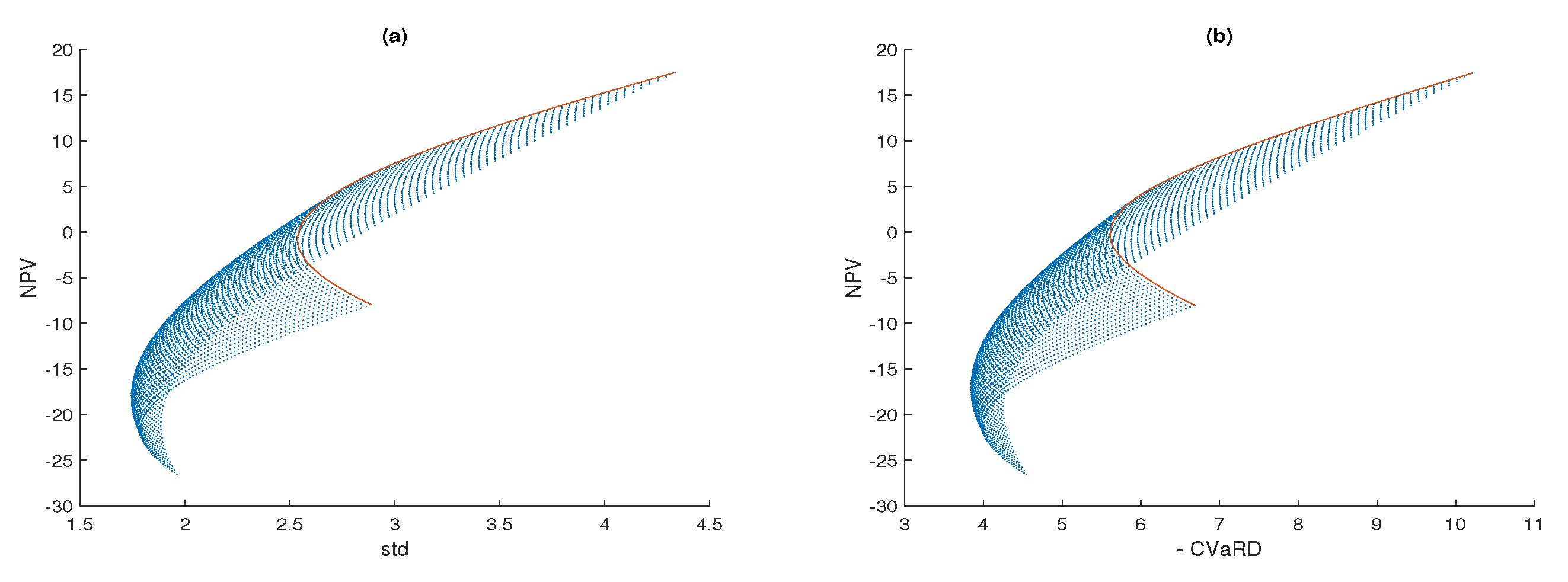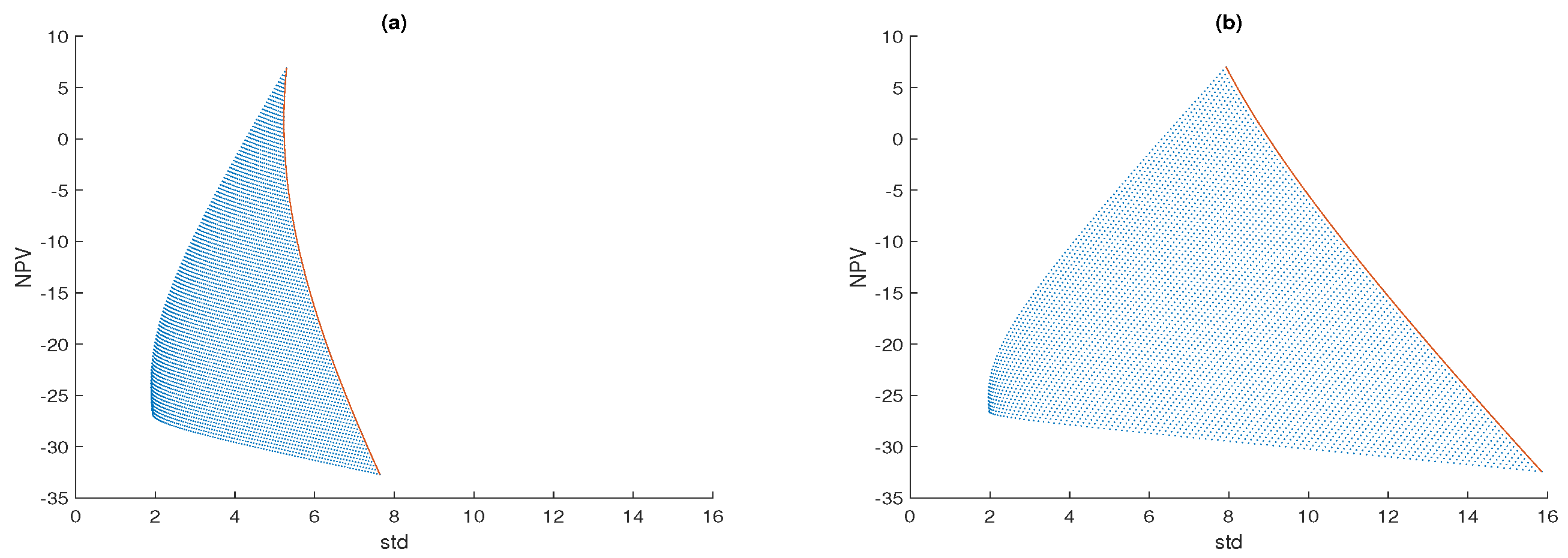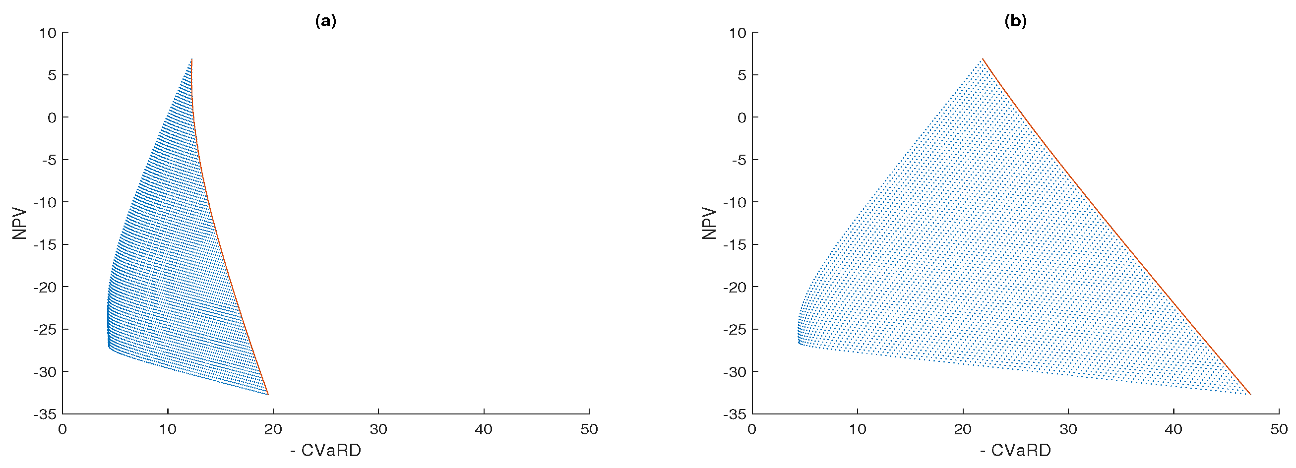Figure 1 depicts opportunity sets for the portfolio selection problem based on the stochastic NPV metric. Frontiers are determined for both risk measures, the standard deviation and the CVaR deviation of the stochastic NPV. Opportunity sets are drawn for both the three-asset (gas, coal, and nuclear power) and the two-asset (gas and coal) portfolio selection problem. Two-asset portfolio opportunity sets are depicted as continuous red lines. When the stochastic NPV metric is used under the CVaRD risk measure, the expected NPV is plotted versus minus CVaRD (i.e. −CVaRD), since adverse events are those with lower NPV values.

The single asset gas portfolio shows the highest values of both risk measures. Such a portfolio is the most profitable and the most risky portfolio. On the other side, nuclear power generation is the less profitable and the less risky option. The efficient frontier, i.e., the locus of power portfolios with the same risk but maximum expected NPV, is represented by the upward sloping curve starting from the minimum risk portfolio and ending to the single asset gas portfolio. It is composed by power generating portfolios that efficiently combine gas, coal, and nuclear generation assets.

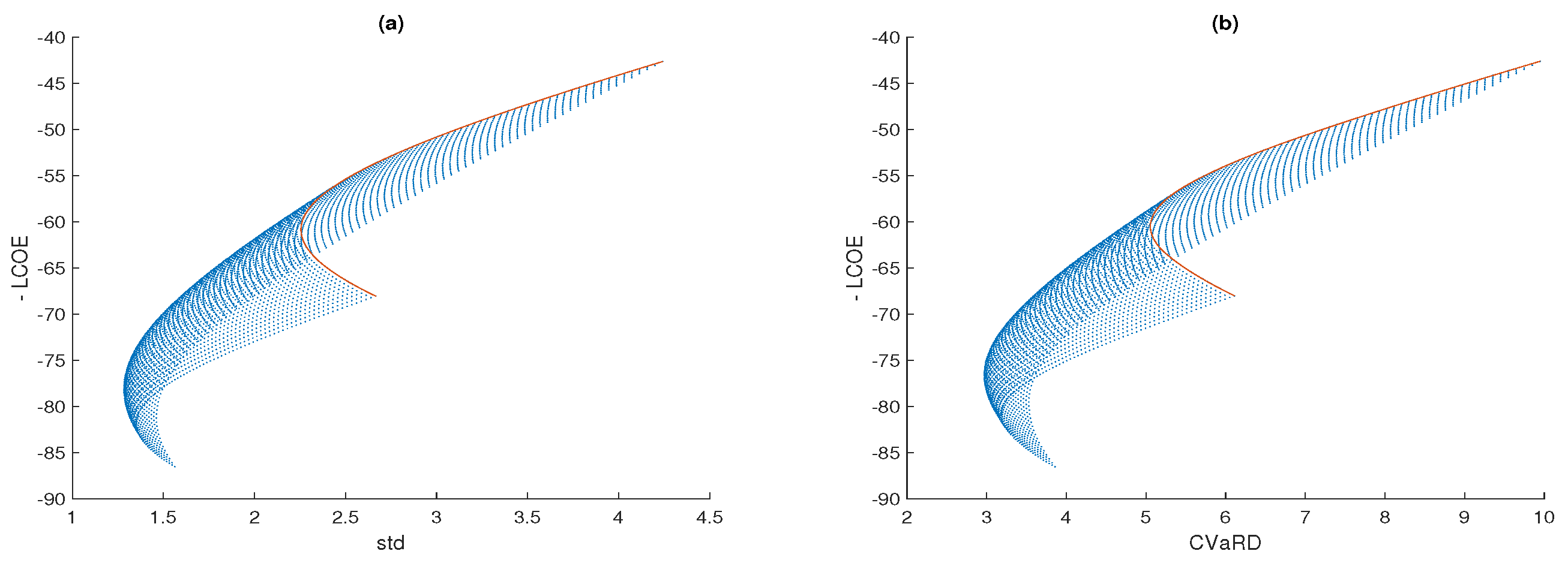
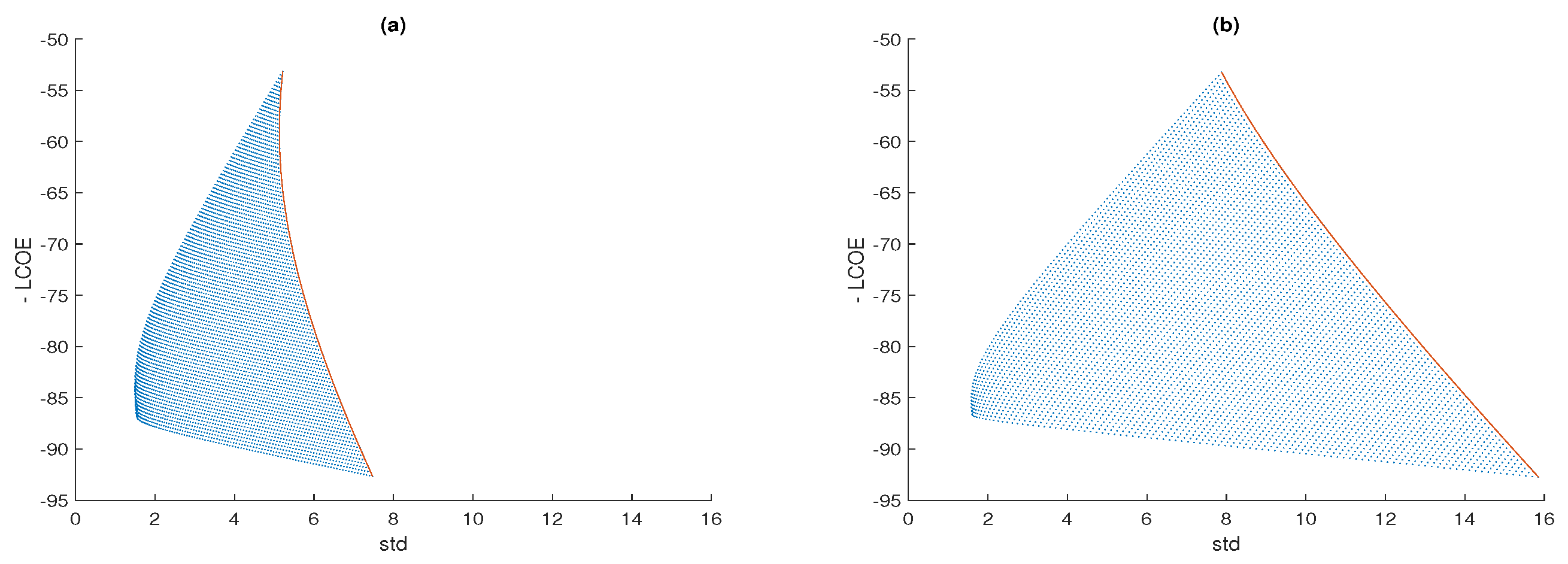
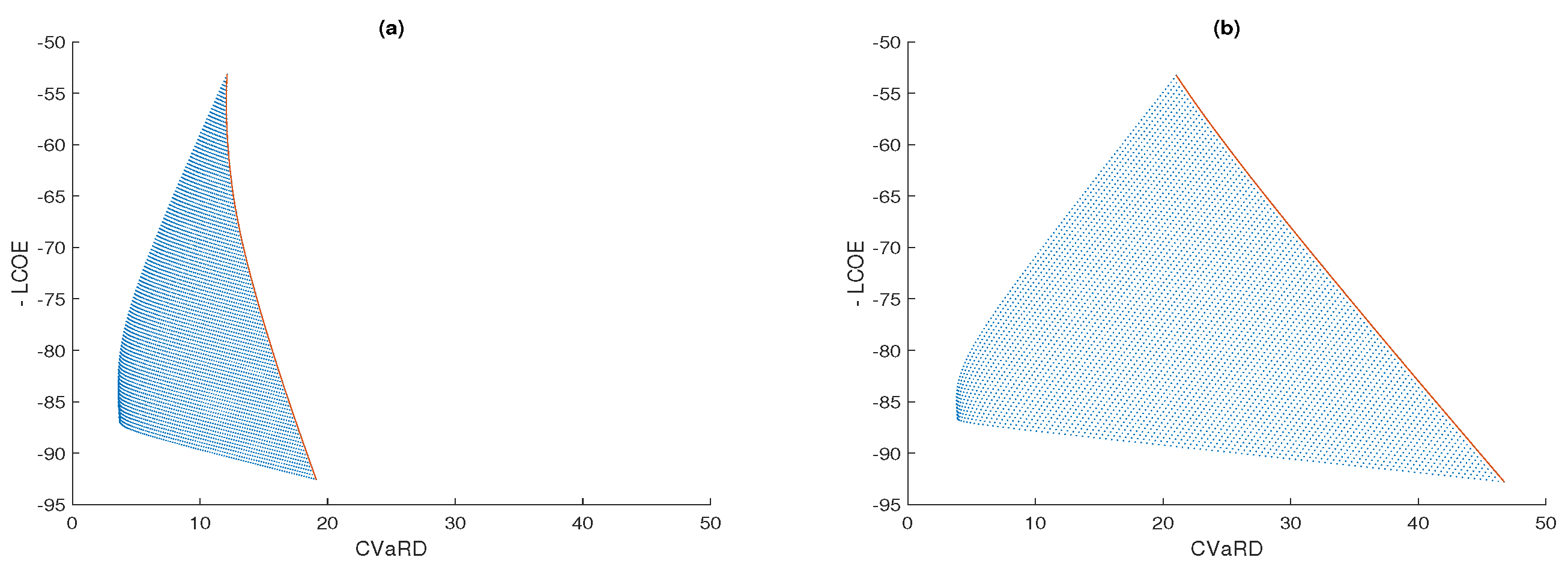
Figure 2 depicts opportunity sets for the portfolio selection problem based on the stochastic LCOE metric. Opportunity sets are determined for both risk measures, namely the standard deviation and the CVaR deviation of the stochastic LCOE. Opportunity sets are drawn for both the three-asset (gas, coal, and nuclear power) and the two-asset (gas and coal) portfolio selection problem. Two-asset opportunity sets are depicted as continuous red lines.

In this case, too, the single asset gas portfolio shows the highest values of both risk measures. Such a portfolio is the less costly and the most risky portfolio [29]. On the other side, nuclear power generation is the most costly and the less risky option. The efficient frontier, i.e., the locus of power portfolios with the same risk but minimum expected LCOE, is represented by the upward sloping curve starting from the minimum risk portfolio and ending to the single asset gas portfolio. It is composed by power generating portfolios which efficiently combine from the cost side gas, coal, and nuclear generation assets.

Table 5. The composition of minimum risk portfolios in the 30-year portfolio selection problem. The two-asset case.

Risk Measure	Metric	${\mathit{w}}^{\mathbf{ga}}$	${\mathit{w}}^{\mathbf{co}}$
std	NPV	29%	71%
	LCOE	29%	71%
CVaRD	NPV	31%	69%
	LCOE	31%	69%

and

Table 6. The composition of minimum risk portfolios in the 30-year portfolio selection problem. The three-asset case.

Risk Measure	Metric	${\mathit{w}}^{\mathbf{ga}}$	${\mathit{w}}^{\mathbf{co}}$	${\mathit{w}}^{\mathbf{nu}}$
std	NPV	9%	24%	67%
	LCOE	9%	24%	67%
CVaRD	NPV	11%	26%	63%
	LCOE	11%	27%	62%

report the composition of minimum risk portfolios, as measured by standard deviation and CVaR deviation, respectively, in the two-asset and in the three-asset portfolio selection problem.

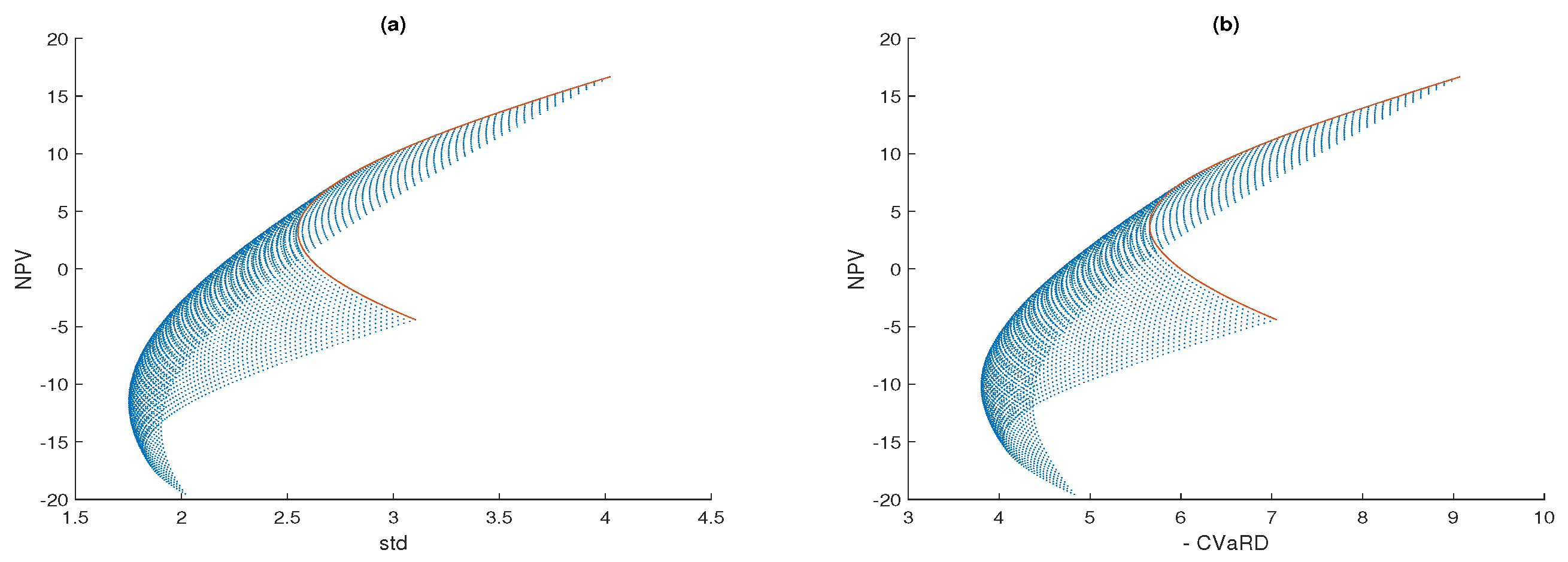
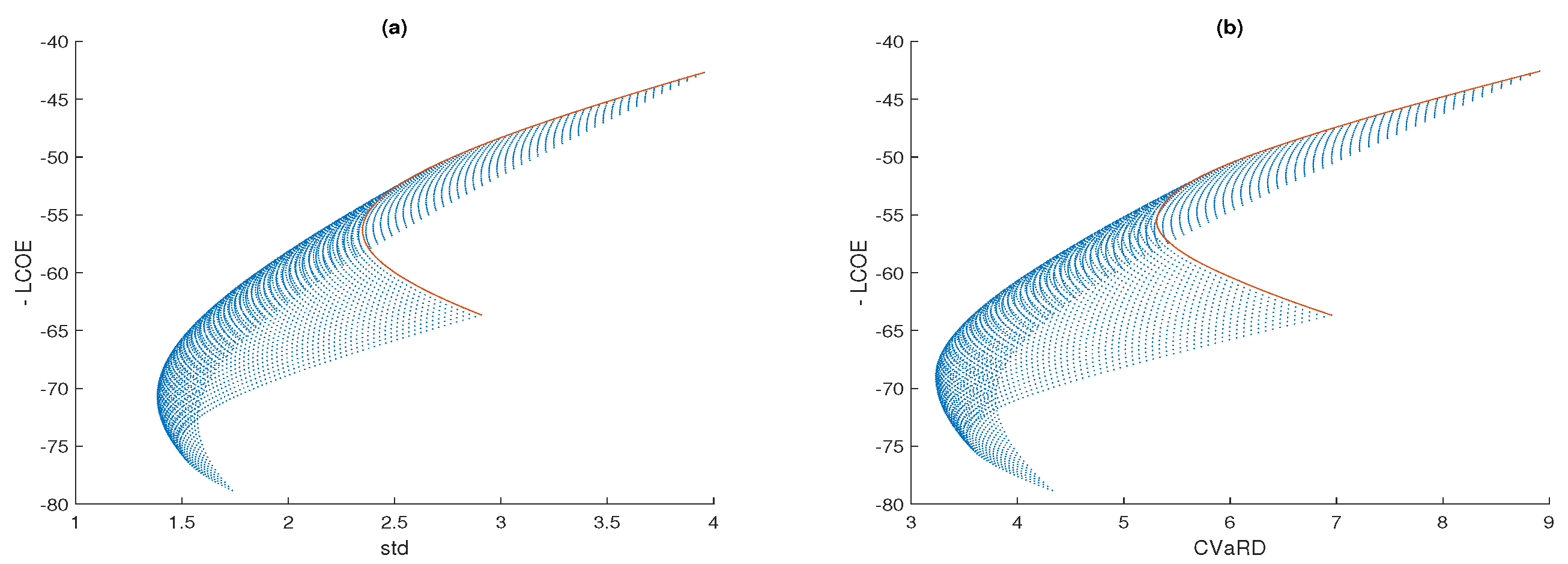
The forty-year portfolio selection problem is depicted in Figure 3 for the stochastic NPV metric, and in Figure 4 for the stochastic LCOE metric.

Table 7. The composition of minimum risk portfolios in the 40-year portfolio selection problem. The two-asset case.

Risk Measure	Metric	${\mathit{w}}^{\mathbf{ga}}$	${\mathit{w}}^{\mathbf{co}}$
std	NPV	35%	65%
	LCOE	35%	65%
CVaRD	NPV	37%	63%
	LCOE	38%	62%

and

Table 8. The composition of minimum risk portfolios in the 40-year portfolio selection problem. The three-asset case.

Risk Measure	Metric	${\mathit{w}}^{\mathbf{ga}}$	${\mathit{w}}^{\mathbf{co}}$	${\mathit{w}}^{\mathbf{nu}}$
std	NPV	12%	23%	65%
	LCOE	12%	23%	65%
CVaRD	NPV	15%	26%	59%
	LCOE	16%	25%	59%

report the composition of minimum risk portfolios.

Let us examine, first, the portfolio selection problem under the standard deviation risk measure. Since revenues for baseload generation do not depend on the power portfolio composition, the stochastic independence between revenues and costs makes efficient portfolio frontiers invariant with respect to the stochastic metric adopted. In such a case, the portfolio selection problem can be performed using the stochastic LCOE metrics, as well as the stochastic NPV metric, thus obtaining the same solution. Minimum risk portfolios, as well as efficient portfolios, i.e., power portfolios belonging to the efficient frontiers, do not depend on the used metric (stochastic NPV or LCOE). A NPV efficient portfolio is also a LCOE efficient portfolio, and vice versa. Such a result does not hold if the CVaRD risk measure is used. However, if the standard deviation of annual revenues is not too high (${\mathsf{\Sigma }}_b=0.10$ in this analysis), the efficient frontier invariance is a very good approximation. As shown in Table 5, Table 6, Table 7 and Table 8, the composition of minimum CVaRD portfolios under both metrics are very slightly different. From this point of view, a cost-based portfolio analysis provides an almost identical solution of that obtained by performing a NPV-based analysis.

Figure 1, Figure 2, Figure 3 and Figure 4 show that some efficient portfolios have negative expected NPV values. This means that for such portfolios the break-even cannot be reached because the expected LCOE is greater than $E\left[{\widehat{P}}^b\right]$. For example, all the minimum risk portfolios derived in the thirty-year case have negative expected NPVs.

Table 9. The composition of efficient portfolios with zero expected NPV. The two-asset case. The composition is the same under both the standard deviation and the CVaR deviation risk measures.

Plant Lifetime	${\mathit{w}}^{\mathbf{ga}}$	${\mathit{w}}^{\mathbf{co}}$
30-year	32%	68%
40-year	21%	79%

depicts the composition of efficient portfolios with zero expected NPV in the two-asset portfolio selection problem.

Table 10. The composition of efficient portfolios with zero expected NPV. The three-asset case. The composition is the same under both the standard deviation and the CVaR deviation risk measures.

Plant Lifetime	${\mathit{w}}^{\mathbf{ga}}$	${\mathit{w}}^{\mathbf{co}}$	${\mathit{w}}^{\mathbf{nu}}$
30-year	40%	48%	12%
40-year	40%	33%	27%

shows the composition of efficient portfolios with zero expected NPV in the three-asset case. The composition of zero expected NPV efficient portfolios is the same under both the standard deviation and the CVaR deviation risk measures. From this point of view, the proposed methodology can be used as a powerful tool of analysis for planning investments in new generating technologies paying attention to risk reducing strategies through power sources diversification, without affecting profitability.

Including CO${}_2$ Costs

The inclusion of CO${}_2$ stochastic costs introduces a further source of risk into the analysis. In this section, the impact that stochastic carbon costs may have on the portfolio selection problem is investigated. To this end, it is assumed that CO${}_2$ stochastic costs do not influence revenues. The effects of CO${}_2$ costs on electricity market price are very difficult to forecast, and this possibility is not considered here. CO${}_2$ costs may impact, in fact, not only on the electricity price level but also on its volatility, thus determining correlation between revenues and costs. However, if such effects are small on the long-run, the results discussed in this section provide a good approximation.

Carbon prices, $P_n^{\mathrm{ca}}$ (the suffix ‘ca’ stands for ‘carbon’), expressed in nominal dollars per ton of CO2, are assumed to evolve in time following a GBM of the type,

$$P_n^{\mathrm{ca}}=exp\left({\beta }_0^{\mathrm{ca}}+{\beta }_1^{\mathrm{ca}}n-\frac{1}{2}{\mathsf{\Sigma }}_{\mathrm{ca}}^{2}n+{\mathsf{\Sigma }}_{\mathrm{ca}}{w}_n^{\mathrm{ca}}\right),$$

(35)

where $w_n^{\mathrm{ca}}$ is a Wiener process independent from fossil and nuclear fuel price processes. Two volatility scenarios are considered corresponding to ${\mathsf{\Sigma }}_{\mathrm{ca}}=0.1$ and ${\mathsf{\Sigma }}_{\mathrm{ca}}=0.2$. Such values are chosen in order to depict, respectively, a low volatility scenario and a high volatility scenario. The parameter ${\beta }_0^{\mathrm{ca}}$ is determined assuming an initial CO${}_2$ price equal to 30 ${\$}_{2018}$ per ton, i.e.,

$$exp\left({\beta }_0^{\mathrm{ca}}\right)=A^{\mathrm{ca}},$$

(36)

where $A^{\mathrm{ca}}=30$ ${\$}_{2018}$. To determine ${\beta }_1^{\mathrm{ca}}$, it is assumed that CO${}_2$ expected prices increase at the inflation rate, i.e.,

$${\beta }_1^{\mathrm{ca}}=\pi .$$

(37)

The contribution of CO${}_2$ costs to the stochastic NPV is computed pointwise at the end of each year.

CO${}_2$ costs increase LCOE expected values and reduce NPV expected values. Investments in gas fired power plants show a positive expected NPV also in the presence of CO${}_2$ costs.

Table 11. Expected NPV and LCOE values.

Metric	Gas	Coal	Nuclear
NPV	6.8	−32.6	−26.5
LCOE	53.2	92.6	86.5

reports NPV and LCOE expected values for a thirty-year plant lifetime.

The inclusion of stochastic CO${}_2$ costs increases financial risk. Figure 5 depicts portfolio opportunity sets under the stochastic NPV metric. Frontiers are drawn for both the three-asset (gas, coal, and nuclear power) and the two-asset (gas and coal) portfolio selection problem on a thirty-year time horizon, using the standard deviation as risk measure. Computations are performed assuming that the volatility of CO${}_2$ prices is equal to ${\sigma }^{\mathrm{ca}}=0.1$ (left panel), and ${\sigma }^{\mathrm{ca}}=0.2$ (right panel) on an annual basis.

Figure 6 shows power portfolio opportunity sets under the stochastic LCOE metric using the standard deviation as a risk measure.

The inclusion of CO${}_2$ stochastic costs makes coal generation the riskiest investment option in both the CO${}_2$ price volatility scenarios ${\sigma }^{\mathrm{ca}}=0.1$ and ${\sigma }^{\mathrm{ca}}=0.2$. As shown in Figure 5 and Figure 6, this happens under both the stochastic NPV metric and the stochastic LCOE metric. If power prices and CO${}_2$ costs are assumed to be independent, the efficient portfolio frontier is invariant with respect to the stochastic metric used. Efficient portfolios under the stochastic NPV metric are efficient also under the stochastic LCOE metric, and vice versa.

Table 12. The composition of minimum variance portfolios: The two-asset case.

${\mathit{\sigma }}^{\mathbf{ca}}$	Metric	${\mathit{w}}^{\mathbf{ga}}$	${\mathit{w}}^{\mathbf{co}}$
0.1	NPV	86%	14%
0.1	LCOE	86%	14%
0.2	NPV	100%	0%
0.2	LCOE	100%	0%

and

Table 13. The composition of minimum variance portfolios: The three-asset case.

${\mathit{\sigma }}^{\mathbf{ca}}$	Metric	${\mathit{w}}^{\mathbf{ga}}$	${\mathit{w}}^{\mathbf{co}}$	${\mathit{w}}^{\mathbf{nu}}$
0.1	NPV	8%	1%	91%
0.1	LCOE	8%	1%	91%
0.2	NPV	4%	0%	96%
0.2	LCOE	4%	0%	96%

report, respectively, the composition of minimum variance portfolios for the two-asset and for the three-asset portfolio selection problem in both volatility scenarios. As expected, the composition of the minimum variance portfolio is the same.

Let us examine the impact of CO${}_2$ price volatility on the portfolio selection problem. First, the two-asset case is discussed. In the presence of stochastic CO${}_2$ costs, the coal component of the minimum variance portfolio reduces as the CO${}_2$ price volatility increases. When ${\sigma }^{\mathrm{ca}}=0.2$, the minimum variance portfolio is fully composed by the natural gas generation asset. As a consequence of the coal component reduction, all minimum variance portfolios show positive expected NPVs. In the three-asset portfolio selection problem, the inclusion of CO${}_2$ costs reduces both the gas and the coal components and increases the nuclear share of power generation of the minimum variance portfolio. In this case, when ${\sigma }^{\mathrm{ca}}=0.2$, the minimum variance portfolio is composed by only two generation assets, namely the natural gas and the nuclear power generation assets. However, minimum variance portfolios show negative expected NPVs. In both CO${}_2$ price volatility scenarios, the zero NPV efficient portfolio is characterized by a natural gas share of about $80\%$ and a nuclear share of about $20\%$.

A similar picture arises also in the case of the CVaR deviation risk measure. Figure 7 shows power portfolio opportunity sets under the stochastic NPV metric, and Figure 8 shows power portfolio opportunity sets under the stochastic LCOE metric, in the presence of CO${}_2$ stochastic costs.

Table 14. The composition of minimum CVaRD portfolios: The two-asset case.

${\mathit{\sigma }}^{\mathbf{ca}}$	Metric	${\mathit{w}}^{\mathbf{ga}}$	${\mathit{w}}^{\mathbf{co}}$
0.1	NPV	93%	7%
0.1	LCOE	94%	6%
0.2	NPV	100%	0%
0.2	LCOE	100%	0%

and

Table 15. The composition of minimum CVaRD portfolios: The three-asset case.

${\mathit{\sigma }}^{\mathbf{ca}}$	Metric	${\mathit{w}}^{\mathbf{ga}}$	${\mathit{w}}^{\mathbf{co}}$	${\mathit{w}}^{\mathbf{nu}}$
0.1	NPV	9%	2%	89%
0.1	LCOE	11%	1%	88%
0.2	NPV	5%	0%	95%
0.2	LCOE	5%	0%	95%

report the composition of minimum CVaRD portfolios for the two-asset and for the three-asset portfolio selection problem in both CO${}_2$ price volatility scenarios, ${\sigma }^{\mathrm{ca}}=0.1$ and ${\sigma }^{\mathrm{ca}}=0.2$. As in the standard deviation case, the coal component of the minimum CVaRD portfolio reduces as the CO${}_2$ price volatility increases. When ${\sigma }^{\mathrm{ca}}=0.2$, it is fully composed by the natural gas generation asset. In this case, too, all minimum CVaRD portfolios show positive expected NPV. In the three-asset portfolio selection problem, the inclusion of CO${}_2$ costs reduces both the gas and the coal components and increases the nuclear share of power generation of the minimum CVaRD portfolio. When ${\sigma }^{\mathrm{ca}}=0.2$, the minimum CVaRD portfolio is composed by only two generation assets, namely the natural gas and the nuclear power generation assets. However, minimum CVaRD portfolios show negative expected NPVs. In both CO${}_2$ price volatility scenarios, the zero NPV efficient portfolio is characterized by a natural gas share of about $80\%$ and a nuclear share of about $20\%$, as in the standard deviation case.

If CVaRD is assumed as a risk measure, the efficient frontier invariance does not hold, even if in our case, the efficient frontier under the stochastic NPV metric and the efficient frontier under the stochastic LCOE metric are almost identical as a consequence of the low value of the standard deviation of annual revenues.

6. Concluding Remarks

The stochastic NPV and the stochastic LCOE are very different evaluation metrics. The first metric accounts for both revenues from selling electricity in power markets and costs incurred during the whole lifetime of each plant in the power generating portfolio. By contrast, the stochastic LCOE is a cost-based metric. If annual revenues are stochastically independent from annual costs, it was shown that efficient frontiers computed using the standard deviation as risk measure are invariant with respect to the used metric. This invariance property is broken in the case of the CVaRD risk measure. However, if the standard deviation of annual revenues is not too high, the invariance of efficient frontiers is a very good approximation. It is worth to underline that the proposed methodology can include also correlation between revenues and costs as, for example, a potential correlation between revenues and natural gas costs, or between revenues and CO${}_2$ costs. However, if such correlation is not too high, the results discussed in this paper hold as a good approximation.

Although the analysis was developed for baseload generation, the proposed methodology can be easily extended also to peak generation. Not only, it can be extended to include renewable power generation with and without energy storage systems. In this last case, i.e. in the absence of storage systems, some hedging mechanism for intermittent renewable generation must be considered. The hedging can be performed at a power system level [18,30] or at a single electricity company level [31]. Moreover, it is worthy to remark that, although the empirical analysis was performed using cost data of new generating technologies, as well as fossil fuel and power prices taken from U.S. markets, spatiality does not affect this methodology. The proposed approach provides, therefore, a powerful tool of analysis to investigate the power portfolio selection problem from a very general and complete perspective. It could offers a quantitative support to electricity companies managers for planning investments in new generating technologies paying attention to risk reducing strategies through power sources diversification, without affecting the profitability of their choices.