1. Introduction
In the United States (US), the residential sector consumes approximately 21% of total energy and generates 19% of all carbon dioxide (CO
2) emissions [
1]. Residential energy consumption is significantly affected by occupant behaviors within their homes [
2,
3]. As a consequence, numerous behavioral intervention methods (e.g., education campaigns, goal setting interventions, and energy-saving incentives) aimed at improving occupant energy use behavior have been studied. Recently, an increasing amount of research has investigated normative messaging interventions, as these interventions have been found to reduce overall household energy consumption and are very cost-effective given its implementation cost (3.3 cents per kWh of electricity saved) [
4,
5,
6,
7]. Normative messaging interventions typically provide households with information about their own energy consumption as well as information about the mean or median energy use of other similar households. The other households’ energy use serves as a descriptive social norm (i.e., a guideline about how other people behave). People feel social pressure to modify their own behavior to fit that of the people around them, especially if they feel similar to those other people [
8,
9]. Thus, a descriptive social norm that conveys that others are energy efficient can motivate high energy consumers to reduce their own consumption to match their peers [
10]. Yet, descriptive social norms can also cause low energy users to increase their consumption by giving tacit permission to match the norm of what their peers are using (i.e., the boomerang effect which refers to unintended consequences of an attempt to persuade resulting in the adoption of an opposing position instead). To mitigate the boomerang effect, injunctive norm messages are frequently added to descriptive normative messages. Injunctive norms convey societal approval or disapproval of a behavior (e.g., a smiley face indicating desirability of low energy use) and have been effective at mitigating the boomerang effect [
10]. From the perspective of electricity utility companies, using normative feedback messages helps reduce overall electricity demand, thus avoiding expensive upgrades to power lines or additional power plant construction. Several large-scale studies in multiple US cities found that normative feedback messages included in monthly or quarterly bills lead to an approximate 2% reduction in energy use (1.4% to 3.3% from approximately 600,000 households [
11] and 1.2% to 2.1% from approximately 170,000 households [
12]). Even small reductions such as this on the aggregate can have a tremendous impact on national energy consumption and thus, net CO
2 emissions.
With norm-based interventions, researchers hypothesize that as reference groups become more personally relevant individuals feel a greater sense of attachment to their group. This connection to the reference group can increase norm adherence and the effectiveness of normative messaging interventions [
8,
13]. Practically, reporting more personalized feedback messages is important because it allows individuals to attend to only what is personally relevant to them [
14]. Until recently, the reference groups in norm-based interventions have been based on geographical proximity (e.g., street and city) and/or housing characteristics (e.g., housing size and heating type) [
5,
11]. Yet, these are not the only characteristics that might inspire feelings of connection between households; other aspects—such as similar lifestyles—may be even more important because of their larger impact on household energy consumption [
15]. Including information about households’ lifestyle in conjunction with geographic and housing characteristics can be used to create more personalized reference groups. Further, because lifestyle information provides insights into when households consume energy, using these reference groups can help individuals learn which time periods offer the most opportunity for them to reduce energy consumption. Nevertheless, more personalized reference group generation has traditionally not been applied as it has been prohibitively costly because of the expense of necessary surveys and home energy audits or extensive manual data collection [
16]. Thus, until recently, personalized normative messaging interventions have not been financially viable on a large scale.
Recent developments and deployment of smart energy metering technology provide new opportunities for behavioral reference group classification as they collected energy consumption data in real-time [
17]. This permits a non-invasive means to generate residential energy use profiles. As energy use profiles are largely dependent on how occupants behave at home, households can be categorized into several normative feedback reference groups based on similar usage patterns [
18,
19,
20,
21,
22]. Thus, by integrating the smart energy metering technology with utility billing systems, it is possible to provide households with the norm of energy profile-based reference groups (i.e., more personalized reference groups) every billing cycle. Further, the non-invasive data collection process makes personalized normative messaging interventions scalable. Unfortunately, although using readily available energy use data permits the creation of personalized normative comparison groups, there has been little understanding of how data granularity and aggregation affect the group categorization performance. In other words, it is still unknown which type of data produces the best reference groups: groups in which members are the most similar to each other. This is important because the typical behavioral pattern of households can change depending on data granularity and aggregation, thus causing different categorization results [
23,
24]. Therefore, the objective of this research is to evaluate the performance of energy profile-based reference group categorization across different temporal granularity and aggregation of energy-use data.
2. Related Works on Electric Energy Consumer Categorization
Studies have used readily available energy use data to find representative behavioral patterns of electric energy consumers for energy tariff structure modelling [
24], building energy use prediction [
25], and renewable electricity generation [
26]. To find representative behavioral patterns, daily energy use profiles for individual energy consumers are created and categorized into several meaningful groups through a clustering analysis. To date, researchers have focused on how profiles should be preprocessed during the categorization process to create more similar groups based on behavioral patterns. The preprocessing step includes reducing the dimensionality of the profiles (e.g., principal component analysis [
26,
27]) and/or transforming the profiles (e.g., min–max normalization [
24,
28] and frequency domain transformation [
29,
30,
31]). Further, several studies [
24,
32] have evaluated the performance of electric energy consumer categorization across different data reduction methods.
In addition to the wide variety of data reduction and transformation methods, researchers [
23,
24] have considered the temporal granularity of energy use data during the categorization process as it can affect group similarity and the number of group members. Specifically, using highly granular data provides more specific information about energy use behaviors of individual electricity consumers and, in turn, will contribute to finding other consumers who are most similar behaviorally [
23,
33,
34]. In contrast, highly granular data may reduce the number of group members, making it difficult to create meaningful groups [
35,
36]. Therefore, the temporal granularity of energy use data should be considered during the categorization process in order to create meaningful groups based on behavioral patterns. Until recently, energy use behaviors of residential and commercial electricity consumers have been represented at a 15-min [
24,
28], 30-min [
26,
37] or one-hour interval [
38,
39]. However, which level of data granularity should be used is still unknown because most studies did not evaluate the categorization performance across time scales. One study [
23] has investigated how data granularity affects the performance of residential electricity customer categorization, but was not without limitation as all clustering results are averaged without accounting for the number of clusters. Since no information is available on the best number of clusters in given datasets, it is necessary to evaluate the clustering performance across different numbers of clusters. Song et al. [
40] examined different temporal granularity levels of residential energy use data as well as the number of clusters during the cluster evaluation process, but did not examine the compound effect of data granularity and aggregation. As a result, it remains unknown which time scale of energy use data produces the best categorization performance.
Moreover, the temporal aggregation of energy use data during the categorization process may improve the similarity within group members [
24]. In general, data aggregation reduces discrepancies in energy consumption caused by irregular changes in a household’s lifestyle (e.g., vacations), which helps more accurately represent typical energy use behaviors. Particularly, as typical energy use behaviors are identified and used for normative comparison group categorization, each household would be categorized into the same energy profile-based groups every intervention cycle. Thus, considering that individuals are more likely to identify with social groups that do not change frequently, the data aggregation would help households have a strong identification with the profile groups. However, data aggregation may not be effective when using long-term data due to significant seasonal changes in energy use behaviors caused by changing weather conditions [
41]. Previous studies aggregated energy use data over one season [
32,
42] or more than six months [
38,
43] to represent typical energy use behaviors of households. Several studies also considered the day types (e.g., weekdays [
32,
38] and all days [
43]). However, the best practice for data aggregation remains unclear as there have been no attempts to compare the clustering performance across different aggregation levels.
After preprocessing the energy use data, various clustering algorithms have been applied to the preprocessed dataset to categorize electricity consumers into meaningful groups. The most widely used clustering algorithms include
k-means [
37,
44], hierarchical clustering [
45] and self-organizing maps [
46,
47]. Recently, several studies have reported the high capability of mean-shift clustering [
48] and mixture model-based clustering [
49] to find representative behavioral patterns of electricity consumers in non-linear or dense datasets. Further, many studies [
43,
50] have evaluated the performance of electricity consumer categorization considering different clustering algorithms because their performance varies depending on data characteristics. However, less effort has been undertaken to investigate how clustering algorithms affect the performance of electricity consumer categorization across different levels of data granularity and aggregation.
3. Behavioral Reference Group Categorization Framework
This research proposes a data mining-based categorization framework using readily available energy use profiles to classify households into highly personalized behavioral reference groups based on their behavioral patterns. The proposed categorization framework considers various levels of data granularity and aggregation while identifying typical behavioral patterns of households. In addition to energy use behavior, we consider housing size during the categorization process as this contributes to significant variations in household energy consumption [
15]. Because all households within normative comparison groups exist in the same climate region, any effects of weather on energy consumption are constant within clusters. By including energy use behaviors in conjunction with housing size and climate region as variables in clustering, energy profile-based reference groups will be more valid for normative comparison.
Figure 1 describes the main process for creating behavioral reference groups based on households’ behavioral patterns. First, data for energy consumption and housing characteristics is preprocessed to improve the clustering performance. Next, clustering algorithms are used for creating personally meaningful reference groups based on households’ energy use profiles. Lastly, clustering performance is evaluated to determine the ideal number of behavioral reference groups.
3.1. Data Preprocessing
The data preprocessing begins with separating households by housing size. Since household energy use is significantly dependent on housing size, comparing energy consumption of household with similar size homes makes more valid behavioral reference groups for normative comparison. Additionally, using public records on housing size permits the creation of behavioral reference groups without any participation of households (i.e., non-invasive manner). In this study, housing size corresponds to the total floor area (m2) of a house. Five categories are created for various house sizes as follows:
HS1: Less than 92.9 m2
HS2: 92.9 to 139.2 m2
HS3: 139.3 to 185.7 m2
HS4: 185.8 to 232.1 m2
HS5: 232.2 m2 or more
The Energy Information Administration (EIA) generally divides housing units into seven housing size categories; this current research uses five categories because using seven categories can create several reference groups with a very low percentage of the total housing units [
51]. Having insufficient members in each reference group undermines the validity of normative comparisons within the group and increases the chance of providing spurious results. For this reason, we combine housing units with less than 92.9 m
2 and more than 232.2 m
2 into two housing size categories, respectively (i.e., HS1 and HS5). This is due to the relatively small number of houses that fall into these two categories; 2.5% of households have less than 46.4 m
2 and 8.3% are between 232.2 to 278.6 m
2 (
Table 1). Combining these groups as such creates an even distribution of households across all housing size categories. On the other hand, this combining process can treat households with small-sized homes (i.e., less than 46.4 m
2 in HS1 and 232.2-278.6 m
2 in HS5) as low energy consumers within their behavioral reference groups. This is because households with small-sized homes account for a small percentage of total households in HS1 and HS5, and generally consume less energy than large-sized homes. Consequently, small-sized homes in HS1 and HS5 may increase their energy consumption when presented with descriptive social norms indicating that other households in their group consume more than them. However, using injunctive norms may prevent households with small-sized homes from increasing their energy consumption when they are treated as low energy consumers in their behavioral reference groups.
After separating households by size, typical behavioral patterns of households are analyzed using different time scales and levels of aggregation. As a data granularity variable, time interval refers to the sampling rate of energy use data, including 15 min, 30 min, one hour, two hours, six hours and twelve hours. The values of time interval have been widely used for representing households’ daily energy use behaviors in previous studies [
23,
37,
38]. The data aggregation variables include monitoring period and day type. The monitoring period denotes the number of weeks: one week, two weeks, three weeks, one month, two months and three months. These values are dependent on messaging cycle (e.g., weekly feedback = all values; monthly messages = one month, two months, and three months) and provide a basis for investigating the short-and long-term effect of data aggregation on the behavioral reference groups categorization. The day type is a variable which consists of weekdays only or all days. If data for energy consumption are collected at a one-hour interval during the weekdays of one week, a typical daily energy use profile is represented in a time-series with 24 time-points by averaging the values for each time interval of the five days (
Figure 2). On the other hand, if energy use date is collected during all days, a typical behavioral pattern is represented by averaging the values for each time interval of the seven days.
Lastly, load shapes are extracted from the typical daily profiles of energy consumption. The load shape extracting process is important because households in a normative reference group should have similar times of energy consumption (i.e., load shapes) but be able to be dissimilar in net energy consumption. In addition, since load shapes represent households’ lifestyles, they should be similar within a behavioral reference group. However, since the clustering process accounts for both the time and volume of energy consumption, households with different patterns of use can be categorized into the same group due to their similar volume of energy use [
24,
28]. For example, although households A and C exhibit different behavioral patterns, they would be categorized into a single group (
Figure 3a). To overcome the adverse effect of volume of the profiles during the categorization process, the three load shape (LS) extraction methods proposed by Song et al. [
45] are adopted because the clustering performance can vary depending on LS:
LS1: Gradient method transforms the existing value of energy consumption (
e) into the rate of change in energy consumption (
erate). It is defined as the change in energy consumption between two consecutive time points (
Figure 3b). The mathematical terms of
erate∗j(
i + 1) can be described by the following equation.
where,
ej(
i + 1) is the amount of energy consumption at time
i+1 for household
j, and
ej(
i) is the amount of energy consumption at time
i for household
j.
LS2: Normalization method transforms the existing values of energy consumption (
e) into the normalized energy consumption (
enorm). It is calculated by normalizing the amount of energy consumption between 0 and 1 (
Figure 3c).
where,
ej(i) is the original amount of energy consumed at time
i,
emin∗j is the minimum amount of energy consumption for household
j,
emax∗j is the maximum amount of energy consumption for household
j.
LS3: Cumulative method transforms the existing values of energy consumption (
e) into the cumulative percentage of energy consumption (
ecper). It is calculated by dividing the cumulative energy consumption at each time by the total amount of daily energy consumption (
Figure 3d).
where,
ecum∗j(i) is the cumulative amount of energy consumption at time
i for household
j and
ed∗j is the amount of daily energy consumption for household
j.
3.2. Application of Clustering Algorithms
To categorize households into personally relevant behavioral reference groups, we applied
k-means clustering (KC), hierarchical clustering (HC), and self-organizing maps (SOM) to the preprocessed dataset for three reasons. First, the performance of the clustering algorithms changes depending on data characteristics [
50,
52]. Consequently, three different clustering algorithms were tested to create more personalized behavioral reference groups. Second, the adopted clustering algorithms do not require prior knowledge on data characteristics. Although other popular clustering algorithms (e.g., mean-shift clustering [
48,
53] and mixture model-based clustering [
49,
54]) have proven useful to categorize objects into several meaningful groups, they make assumptions about how data is distributed within each cluster. Because data distribution as well as the number of clusters in a given dataset of household energy consumption is unknown before the clustering analysis, it is not ideal to apply the assumption-based clustering algorithms for this research. Third, the adopted clustering algorithms have been widely used in the field of identifying representative behavioral patterns of residential and commercial customers [
24].
The KC algorithm partitions objects into
k distinct clusters. The first step of KC is to arbitrarily determine
k initial cluster centers as the initial centroids of groups. Then, each object belongs to the cluster whose centroid is closest to the object (
Figure 4a). If an object
p is apart from the centroid
ci of a cluster
Ci, the sum of Euclidean distances between them can be minimized by the following objective function
E:
This objective function creates k clusters as tightly clustered and unique as possible. Until there is no variation in similarities, the KC reallocates objects to new centroids of clusters and evaluate their quality, using the objective function.
The HC decomposes the given set of data objects and generates a tree diagram, called a dendrogram (
Figure 4b). The HC is implemented in the following four steps: (1) constructs a similarity matrix which correspond to a symmetric matrix representing the distances among all the data objects; (2) defines each object as one cluster; (3) combine the two nearest clusters until there is only a single cluster; and (4) cuts the dendrogram at the proper level which corresponds to the
k clusters.
The SOM projects high-dimensional input data onto a two-dimensional map using an unsupervised network model that consists of an input and output layer (
Figure 4c). In the SOM map, there are connections among the vectors (neurons) in the input and output layer. This connection is dependent on a weighting vector, called the connection intensity. The SOM algorithms consists of the following four steps. First, the Euclidean distance between the input neuron and the weigh vector is calculated. Second, the closest output neuron to the input neuron is found and considered as the best matching unit (BMU). Third, the weight vectors of the BMU and its surrounding area are updated according to Equation (6).
where,
wi(
k) is the previous weight of neuron,
wi(
k + 1) is the new weight of neuron,
ɛ(
k) is the learning rate and
hp(
i,
k) denotes the neighborhood size of the winning neuron
p at an iteration of
k. Fourth, this learning process is continued until a termination criterion is met.
3.3. Clustering Performance Evaluation
The clustering results are evaluated using the Davies–Bouldin Index (DBI) to determine the best number of behavioral reference groups in the given dataset. Many cluster validation indices (e.g., Silhouette Index and Clustering Dispersion Indicator) have been developed for clustering performance evaluation. However, the DBI has proven to be representative of those indices because it is capable of measuring group similarity regardless of data properties (i.e., monotonicity, noise, density and skewed distributions) [
55]. The DBI is one of the most widely used indices in the field of residential energy consumer categorization to not only determine the best number of clusters but also evaluate the clustering performance across different data preprocessing methods [
24,
45] and different clustering algorithms [
24,
48]. For these reasons, researchers [
25,
50,
56] have adopted the DBI as a cluster validation index when solving their clustering problems.
The DBI calculates the relative values to measure the group similarity based on between- and within-cluster variances [
57]. Smaller DBI values indicate better clustering performance; clusters are more tightly knit and have greater distances between each other. The DBI is defined as
where
k: the number of clusters;
di: the average distance between all objects in the
ith cluster and the centroid of the
ith cluster;
dj: the average distance between all objects in the
jth cluster; and
dij: the distance between the centroids of the
ith and
jth clusters. In addition to the group similarity, computational time is evaluated since it can significantly vary depending on data granularity.
4. Data Collection
We collect energy use and housing size data of 3000 households in Holland, Michigan. Each residence has a smart energy meter administered by the Holland Board of Public Works (HBPW). This smart metering technology captured electricity consumption data every 15 min from January 1 through December 31, 2016. The city of Holland experienced four distinct seasons, thus causing 5784 heating degree days (HDD) and 756 cooling degree days (CDD) in 2016 [
58]. In accordance with the HDD and CDD that indicate needs for heating and cooling, energy consumption patterns varied by season (
Figure 5). Since clustering performance can vary depending on data characteristics, clustering one-year electricity consumption data helped to generalize results across different seasons. Additionally, HBPW provides housing size data.
503 households are excluded from the data set as they moved or experienced smart meter failure, causing missing and abnormal energy use data. In this research, households with abnormal energy consumption are defined as homes who have energy consumption data outside of the following range (
Figure 6): Q1−1.5×IQR to Q3 + 1.5 × IQR, where IQR is the interquartile range (i.e., Q3−Q1), Q1 is the first quartile and Q3 is the third quartile of energy use data at a certain time of the day. Additionally, no energy use data was gathered on March 13, 2016 due to a system malfunction with the electrical metering systems. Lastly, no housing size data for 319 households was obtained from HBPW, so these homes were excluded as well. In total, 2248 households are included in the analysis (
Table 2).
5. Results
A clustering analysis is performed using the collected data in conjunction with the proposed categorization framework to investigate the effect of data granularity and aggregation on the behavioral reference group categorization. The proposed categorization framework is coded in MATLAB (R2017b, The MathWorks, Natick, MA, USA) and implemented on an Intel(R) Core(TM) i7-6700 CPU (3.40 GHz) with 16 GB RAM. In order to conduct the clustering analysis under the same condition, we use the same number of households across all the housing size categories since the number of households can affect computational time. As shown in
Table 2, HS5 has the fewest households (i.e., 73), so 73 households are randomly selected from HS1, HS2, HS3 and HS4. Additionally, the cluster
k variable changes from two to ten across all housing size categories. Then, behavioral reference group categorization for each housing size category is performed 52 times with energy use data of 73 randomly selected households during different weekly billing periods of the year. This not only avoids biased clustering results by unequal sample size but also simulates a year-long behavioral intervention that provides normative feedback every week. For each messaging cycle, 72 different types of typical energy use profiles for each household are created for each combination of data granularity and aggregation (i.e., six time intervals by six monitoring periods by two day types = 72 typical daily energy use profiles per household). After applying the clustering algorithms to the preprocessed dataset, we average the clustering results (i.e., DBI and computational time) over different levels of data granularity and aggregation. Lastly, once the most desirable categorization framework is found using DBI values, we identify representative behavioral reference groups for a weekly intervention cycle (i.e., May 9–15, 2016) for two reasons. First, although the categorization framework makes group members the most similar, it is uncertain whether the identified groups are characterized by households’ behavioral patterns and distinguishable from each other. Second, diverse behavioral patterns of residential energy consumers tend to be observed during this period due to the changes of seasons [
40]. Thus, this group identification process enables the testing of how distinguishable groups are in terms of energy use patterns.
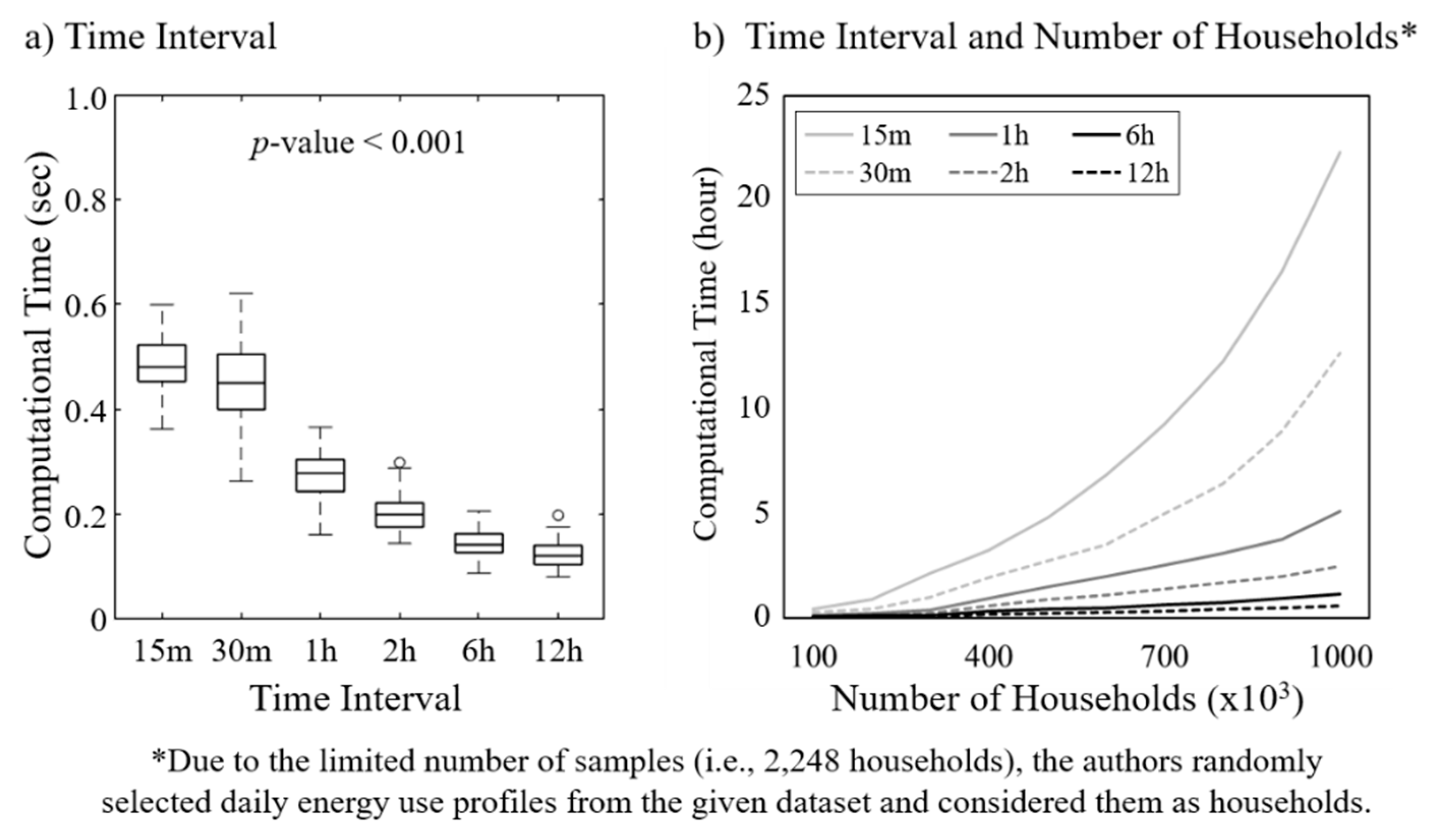
5.1. Clustering Performance by Data Granularity
Representing daily energy use profiles using six-hour intervals produces the lowest average values of DBI except for when three and eight behavioral reference groups are created based on the profiles (
Figure 7). The higher average values of DBI are found when using less granular data. When investigating the average values of DBI by time interval across different load shape extraction methods, using six-hour intervals in conjunction with LS1 generally produces the lowest average values (
Figure 8a). However, the clustering results using LS2 and LS3 show that the lowest average values of DBI are observed with six-hour and 12-h intervals. Additionally, regardless of which clustering algorithm is applied (KM, HC, or SOM), the lowest average values of DBI are obtained from clustering analysis using six-hour intervals (
Figure 8b).
The computational time decreases when behavioral reference groups are created based on less granular energy use data (i.e., six and twelve hours) as would be expected (
Figure 9a). As the number of households increases, the data granularity makes the difference in computational time exponentially larger (
Figure 9b). This significant increase in computational time exists for all the clustering algorithms (
Figure 10).
5.2. Clustering Performance by Data Aggregation
Aggregating energy use data over twelve weeks produces the lowest average values of DBI across all the number of clusters (
Figure 7). The average values of DBI decrease with longer monitoring periods. Looking closely at the average values of DBI by monitoring period across different load shape extraction methods, more aggregated data (i.e., twelve weeks) produce the lowest average values of DBI in case of LS1 (
Figure 11a). However, the clustering results using LS2 and LS3 show that the average DBI values do not vary by monitoring period. In addition, regardless of clustering algorithms, aggregating energy use data over twelve weeks produces the lowest average values of DBI (
Figure 11b).
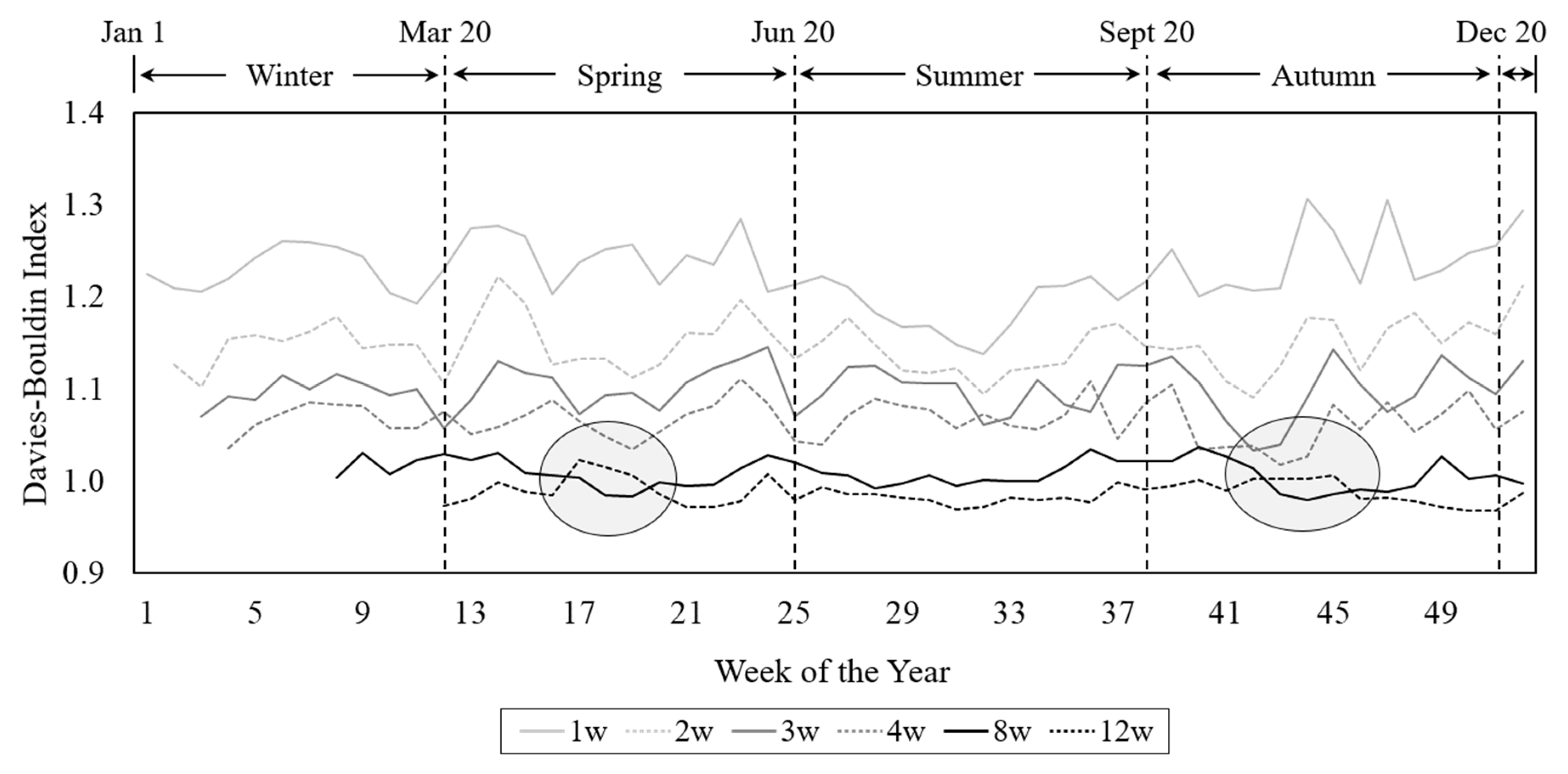
Across different intervention cycles, aggregating energy use data over twelve weeks generally produces the lowest average values of DBI except for the middle of Spring and Autumn (
Figure 12). The average values of DBI tend to decrease with longer monitoring periods.
There is no difference in the average DBI values by day type (
Figure 7). When investigating the average values of DBI by day type across different load shape extraction methods, more aggregate data (i.e., all days) in conjunction with LS2 and LS3 produce the lowest average values of DBI (
Figure 13a). In contrast, the clustering results using LS1 show that aggregating energy use profiles over weekdays produces the lowest average values of DBI. Further, across all the clustering algorithms, the average values of DBI do not vary by day type (
Figure 13b).
5.3. Overall Clustering Performance
Figure 14 shows the results of the clustering analysis considering data granularity and aggregation, load shape extraction methods, and clustering algorithms. The lowest average value of DBI is achieved under the following conditions: (1) data granularity of six hours, (2) data aggregation over all days of twelve weeks, (3) load shape extraction by LS3, and (4) application of hierarchical clustering algorithm to find the ideal number of clusters.
5.4. Behavioral Reference Group Identification
Using three energy profile-based groups produces the lowest DBI values in housing groups HS1 and HS5 (
Figure 15). For housing groups HS2, HS3 and HS4, four energy profile-based groups produce the lowest DBI values. Considering that two groups in HS4 and HS5 show similar behavioral patterns of households, the identified groups have five distinguishable daily energy use profiles (
Figure 16). Households in Group 1 consume energy mostly in the evening. Households in the Group 4 consume energy mostly in the morning. The energy use profiles are also contingent on the housing size category.
6. Discussion
Since lower values of DBI indicate higher intra-class similarities and lower inter-class similarities within a group, it is clear that capturing typical daily energy use profiles of households using a six-hour interval leads to the most similar behavioral reference groups in terms of DBI (
Figure 7). These results are be supported by the following two conflicting observations. First, the sparsity of data points in a group increases with higher dimension of data [
35,
36]. Thus, behavioral reference groups may not be meaningful for normative comparison in a highly dimensional space. Second, groups become more distinguishable as the number of data attributes increase.
The computational efficiency of the group categorization process decreases when using less granular data (i.e., 6 h and 12 h). Time to create groups increases exponentially with more households. This exponential increase is attributed to the linear time complexity of the KC and SOM with respect to the number of data objects [
59] (
Table 3). Clustering a small number of data objects shortly converge clustering results to the global optimum after twelve iterations [
60]. However, when using a large number of data objects, these clustering algorithms make the number of iterations larger and then cause longer computational time for the convergence process. For the HC, the time complexity is quadratic or worse depending on the number of data objects [
61].
Moreover, it appears that aggregating energy use data over longer monitoring periods (i.e., twelve weeks) makes behavioral reference groups more similar (
Figure 7). These results align with the previous findings that the aggregation periods should be long enough in the same seasonal context to represent typical daily energy use profiles for each electricity customer [
24]. Interestingly, using 8-week aggregate energy use data produces the lowest average values of DBI in the middle of Spring and Autumn (
Figure 12) when the weather is shifting from warm to cold and vice versa. These results can be expected because households tend to exhibit similar energy use behaviors within the same season but different behaviors while seasons are changing (e.g., April to May) [
41]. Thus, as the monitoring periods include more days that correspond to this period, using less aggregated energy use data (i.e., eight weeks) produces the lowest average values of DBI.
Further, the similarity of households in behavioral reference groups does not vary by day type (
Figure 7). This conflicts with previous studies that suggested aggregating energy use data over all days of the given monitoring period (e.g., season or year) could interrupt typical energy use patterns of households [
24,
38,
44]. However, these clustering results are understandable because households are likely to consume different amounts of energy but exhibit similar behavioral patterns (i.e., load shape) [
20,
41,
62] and not all regions have similar heating and cooling loads as Holland, Michigan. Consequently, considering weekdays and weekends together contributed to creating typical daily energy use profiles and make behavioral reference groups more meaningful.
Figure 14 presents the most desirable behavioral reference group categorization framework for normative comparison. This framework not only increases the similarity of households in behavioral reference groups, but also makes the groups distinguishable based on daily energy use profiles (
Figure 16). Using six-hour intervals will make behavioral reference groups more personalized and require a relatively short computation time. However, this does not mean that energy use data should be sampled from smart meters at a six-hour interval. This is because different data granularity can be required for other energy saving purposes in the residential sector. For example, using high-resolution energy use data makes it possible to predict and avoid daily peak demand in homes [
63]. Therefore, instead of setting a low data sampling rate, we recommend collecting highly granular energy use data from smart meters and then change the data granularity to six-hour intervals when creating more personally relevant comparison groups.
Additionally, when a normative messaging intervention is deployed to one million homes, using six-hour intervals does not create a feedback lag (it takes approximately two hours for their categorization). However, if household energy use profiles were clustered at a large spatial scale (e.g., state, climate region) to improve the validity of normative comparison with sufficient group members, this could cause a latency of normative behavioral feedback despite using six-hour intervals. Coupling parallel computing techniques with the proposed categorization framework solves this computational issue (e.g., it is 30 times faster for image dataset categorization [
64]). Further, aggregating energy use data over all days of twelve weeks makes behavioral reference groups more similar. A data aggregation issue might arise due to the large volume of historical data that must be stored and processed in databases to create more personally relevant comparison groups. As mentioned by Kaisler et al. [
65], the existing database management systems operated by utility companies may be unable to solve such storage and processing issues due to their limited capacity. This will, in turn, be a barrier to create more personally relevant comparison groups by aggregating energy use data over all days of twelve weeks. However, big data technologies (e.g., cloud computing) have been widely adopted as a means for implementing the smart grid and continue to become more widespread [
66,
67]. In addition to the data storage and processing issues, data aggregation process may have difficulty creating typical energy use profiles when home energy use data has outliers at certain times. This is important because outliers make mean values biased toward them, and thus are not representative of given data. While we removed households with outliers from this analysis, electricity utility companies would include all residential customers in normative feedback programs for overall electricity demand reduction. Therefore, it is recommended that the data aggregation process involves removing outliers and averaging the values of remaining energy use data to create typical daily energy use profiles.
Future research should identify personalized behavioral reference groups within a seasonal context. While using more aggregated and less granular data creates more personalized behavioral reference groups, households can be provided with the norm of different reference groups every billing cycle if they change behavioral patterns. Considering that individuals do not strongly identify with social groups that they can easily join and leave (e.g., people who live in temporary housing such as military family homes does not have a strong identification with their neighbors [
68,
69]), frequent changes in behavioral reference groups may weaken the households’ identification with those groups. Therefore, understanding how frequently individuals change their energy use behaviors will allow interveners to not only find an appropriate categorization cycle but also provide suitable comparison groups across all seasons. Additionally, future work should investigate how households perceive their energy profile-based reference groups, since compliance with social norms depends on residents’ identification with those groups [
70]. Unlike traditional geographic proximity-based groups (e.g., neighbors) whose members may know each other, residents in energy profile-based groups are not expected to know each other on a personal level. Thus, this could make it difficult for residents to feel strongly attached to other members of the profile-based groups. However, individuals regularly build social relationships with others in online communities (e.g., movie-related communities, online gaming) despite a lack of physical contact [
71,
72,
73]. Sharing not only the characteristics of groups but also member behavior makes people feel more attached to their online communities [
71]. Therefore, despite limited physical contact among the members of energy profile-based groups, by highlighting similar patterns of behavior, interveners can encourage residents to strongly identify with their profile group and thus adhere to group norms.
7. Conclusions
Recent advances in energy monitoring technology provide new opportunities to construct more personalized feedback messages by constructing energy-use profiles of consumers on a large scale. The creation of meaningful personalized reference groups based on similar behavioral patterns of households can lead to increases in social norm adherence and thus, improvements in normative messaging intervention effectiveness. However, previous research efforts had two limitations: uncertainties about the role of temporal granularity in group categorization performance and uncertainties about the ideal aggregation of energy use. Therefore, this research evaluates the performance of behavioral reference group categorization across different levels of temporal granularity and aggregation of energy-use data.
Reducing the temporal granularity of energy-use data (i.e., six-hour intervals) creates personalized behavioral reference groups while minimizing computational time, as compared to more granular data intervals. These results are consistent regardless of load shape extraction method and clustering algorithm. Additionally, aggregating energy use data (i.e., across all days of twelve weeks) generally increases the similarity of behavioral reference groups. Data aggregation effects decreases only when seasons change. Also, the compound effect of data granularity and aggregation varies depending on load shape extraction method and clustering algorithm. Using more aggregated but less granular data results in further improvement in the similarity of behavioral reference groups by cumulative percentage-based load shape extraction in conjunction with hierarchical clustering. These results provide a guideline for norm-based energy conservation interventions, specifically for households in Holland and residential areas with similar energy use patterns: energy-use profiles should be categorized after aggregating energy-use data across all days of twelve-weeks using six-hour increments.
This research contributes to the literature by enhancing our knowledge of how the temporal granularity and aggregation of energy use data affects the similarity of behavioral reference groups in terms of energy use profiles. Creating energy profile-based reference groups with higher similarity among group members will help maximize the effectiveness of residential energy use normative feedback interventions. In addition, this research establishes a data mining-based categorization framework to classify households into several personalized normative comparison groups. With this categorization framework, it is possible to generate personally relevant normative comparison groups in a non-invasive manner and likely increase normative feedback effectiveness. The proposed categorization framework provides interveners with a scalable option for creating personalized normative feedback messages.


