The Latest Method for Surface Tension Determination: Experimental Validation

Abstract

The highest effectiveness of heat exchange is under boiling; hence, surface tension is an important parameter and should be determined when new liquid substances are created. The most popular methods are based on numerically solving the Young–Laplace equation by applying the Bashforth and Adams algorithm, which fails at the poles and at the inflection points. The newest algorithm is based on the closed-form expressions that define a drop or bubble. It gives the accurate solutions for the fully created drops or bubbles. To validate it, the surface tension value is determined for the air bubbles in water and compared with the reference data. Because the relative discrepancies are extremely small, the new method may be thought of as positively validated.

1. Introduction

A necessity to increasing the effectiveness of energy transfer results in heat exchange under boiling conditions [1]. Hence, heat transfers across a free surface, which means that surface tension must be included into an analysis. Since new created substances take part in energy transfer, they thermodynamic properties, including surface tension, must be determined. In addition, surface tension is one of the parameters that determine the combustion efficiency [2,3,4,5]. It is also an important property of the new synthesized surfactants that are applied during the fuel processing [6,7]. Moreover, surface tension impacts on the hydraulic characteristics of transporting equipment [8]. Since clouds contain extremely small the water drops and ice particles, the surface effects should be taken into consideration [9,10,11,12]. In the last case, research is conducted for supercooled water [13].

The majority of commonly used methods for determining surface tension originate from an equation that was described by Young [14] and derived by Laplace (1806) (cf. Adamson [15])

$$\Delta p=\gamma \left(\frac{1}{R_1}+\frac{1}{R_2}\right),$$

(1)

where:

Δp - pressure difference between two sides of interface in the bulk phases [Pa];

γ - surface tension [N/m];

R₁, R₂ - the main radii of curvature [m] (cf. Figure 1).

Since Young–Laplace Equation (1) does not contain any coordinate of an interface shape, Bashforth and Adams [16] proposed a numerical algorithm for its solution. The algorithm, which possesses numerous modifications (e.g., [17,18,19,20,21,22,23,24,25,26,27]), is a Cauchy problem and is applied to determining either an interface shape or surface tension value.

However, the algorithm fails when surface tension is determined from a spherical drop (e.g., at 24 °C γ = 79.32 ± 0.19 N/m instead of 72.28 N/m), which was thoroughly investigated by Hoorfar and Neumann [28]. As a result of the comprehensive study, Hoorfar and Neumann [28] summarized that the algorithm has an intrinsic problem that cannot be surmounted by the numerical schemes improvements.

What is more, there is another insufficiency that is not discussed whatsoever. This insufficiency consists in the lack of a solution at a sharpened tip and tapering neighborhood. Thus, the algorithm is used only to solve pendant drops, and the solutions for the fully created droplets are not presented. For instance, the treatise on surface tension phenomena by Hartland and Hartley [17] does not show the solutions in the full range from 0° to 180°, in other words, there is no solution at the tapered apex. In addition, there is no chapter on the fully created drops or bubbles. For example, the shapes of the pendant interface are listed from Θ = 10° to 179.064° and from Θ = 179.064° to 0.935678° (cf. on page 170 in Hartland and Hartley [17]) or from Θ = 1° to 6.36988° and from Θ = 6.36988° to 0° (cf. on page 243 in Hartland and Hartley [17]). A lack of solution for Θ = 0° that is at the most distant place from the nozzle should be emphasized. Undoubtedly, this is a place where the two-phase static model assumptions are satisfied in the experimental conditions most.

The Young–Laplace equation is the static two-phase model; hence, the experiment should satisfy these assumptions. Thus, the best experimental approximation is the state when the drop has just been disconnected from the nozzle (i.e., the third solid phase) and there is no flows inside or outside the drop. Although the ultimate cameras containing charge-coupled devices (CCD) are capable to capture the drop at such a moment, the Young–Laplace equation may not be solved at the poles of the drop.

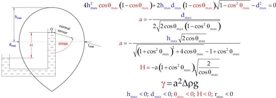
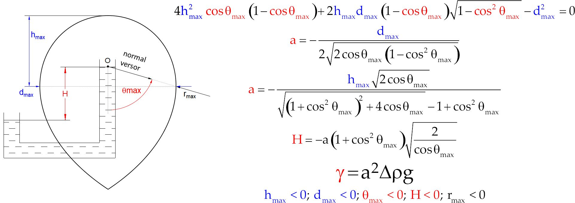
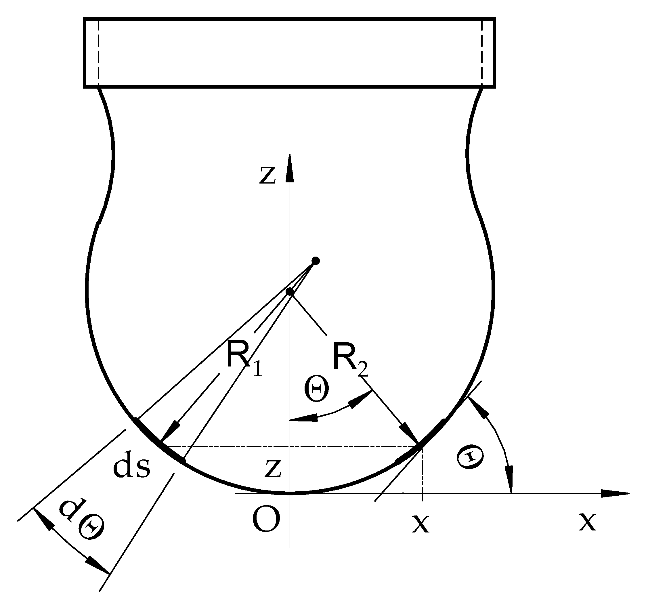
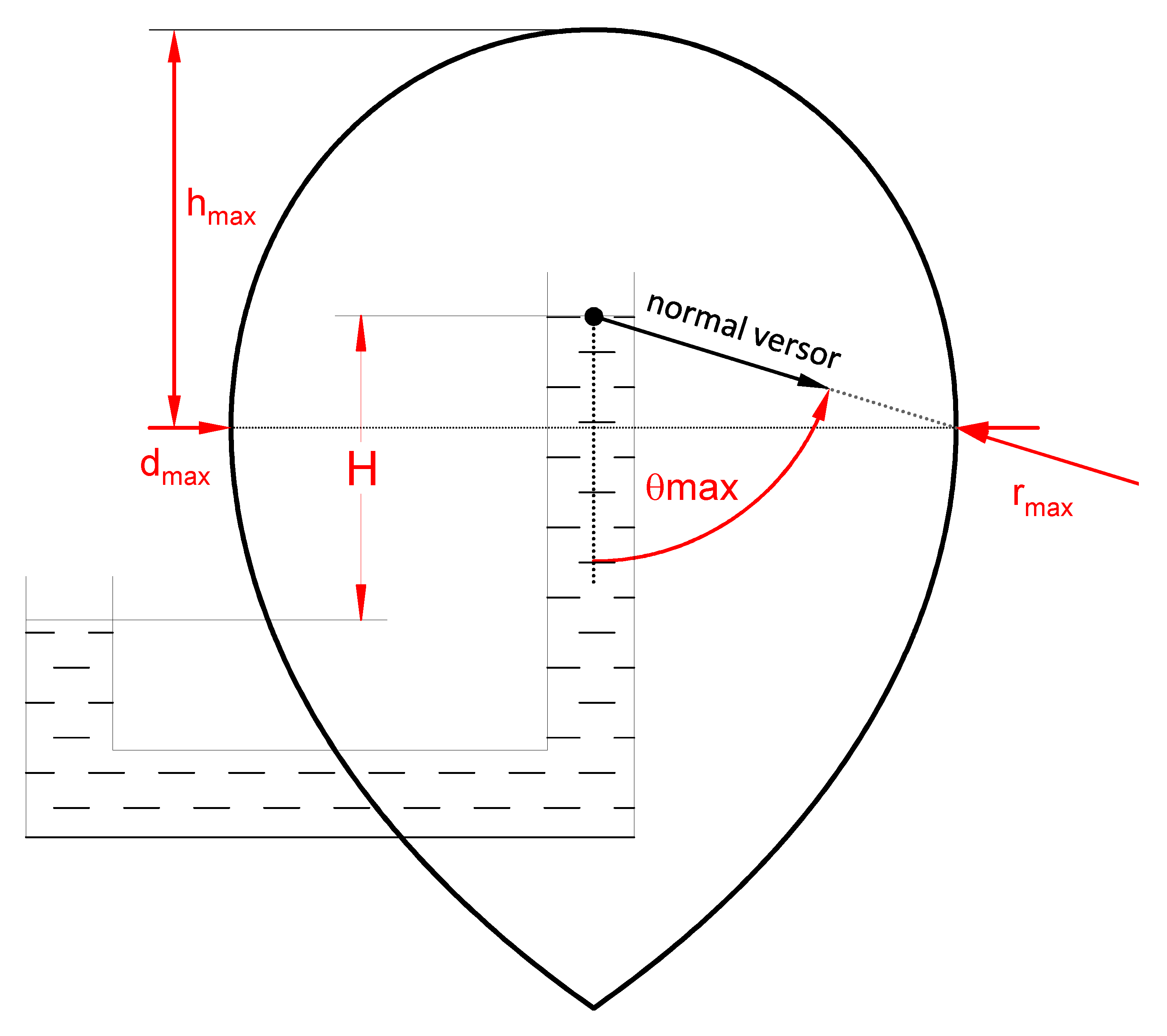
2. Contemporary Interface Model

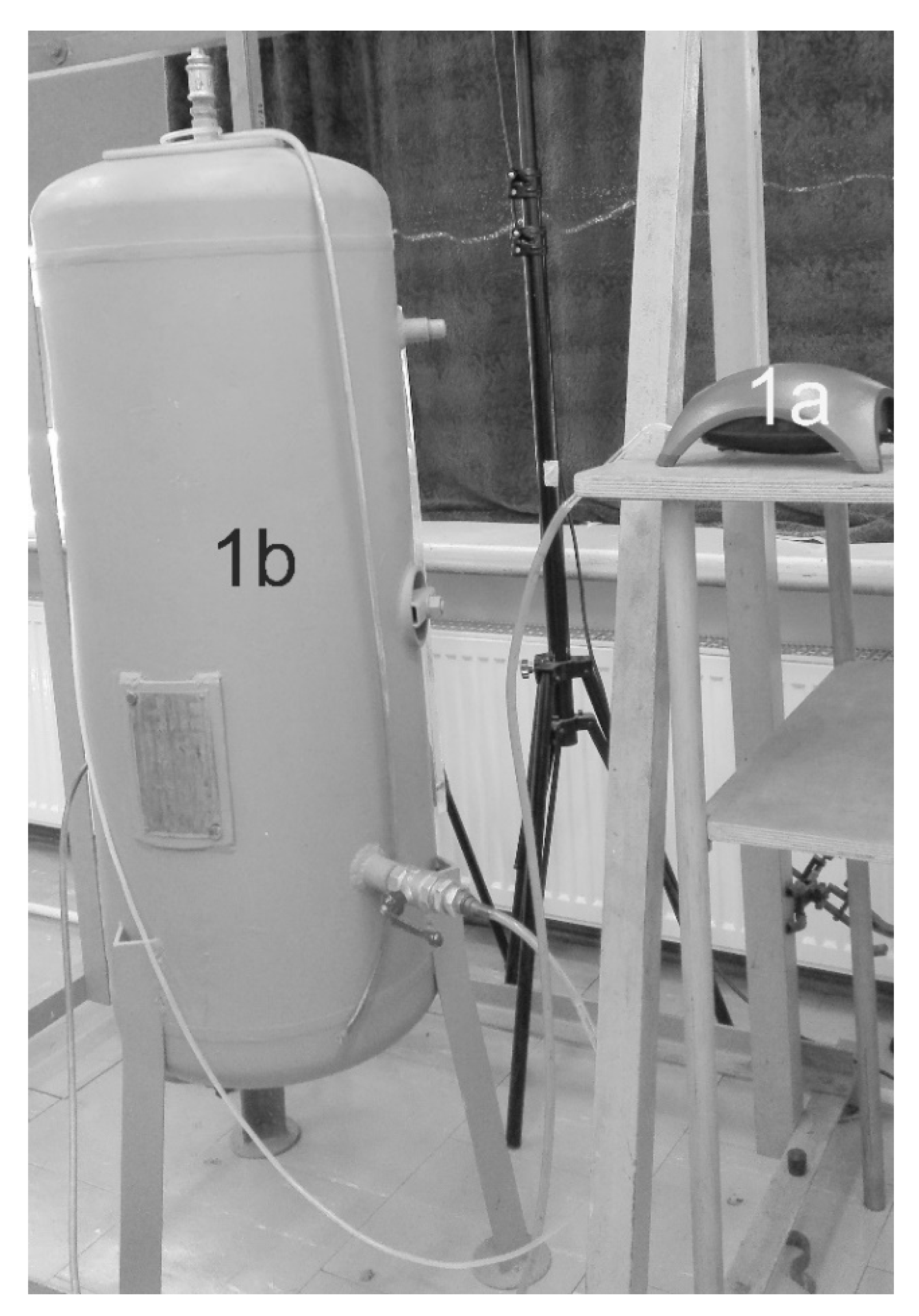
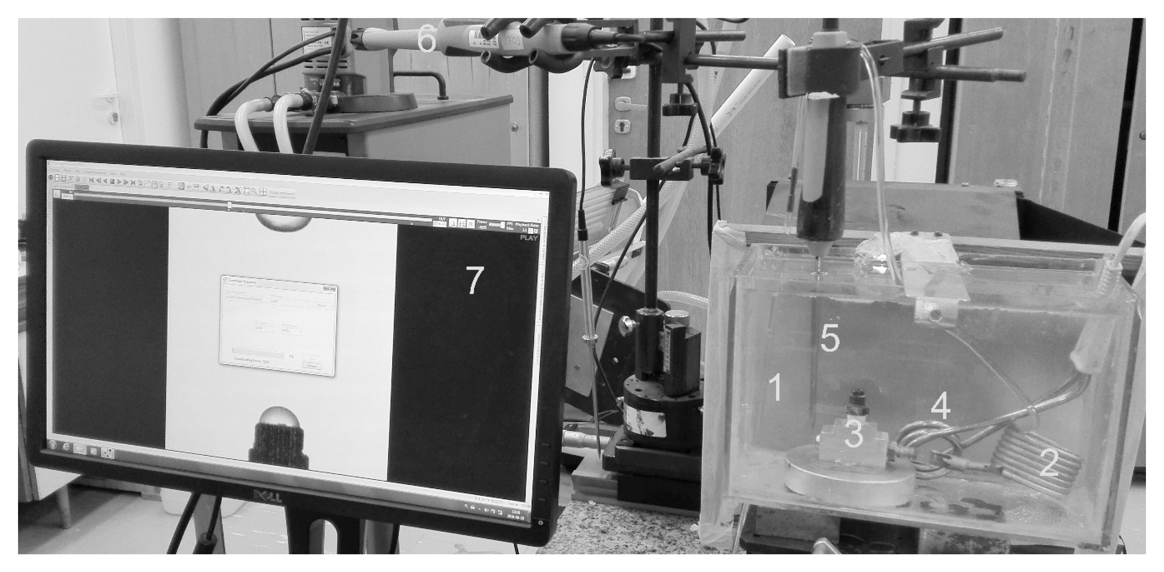
Nevertheless, there are the analytical functions that circumscribe either a drop or bubble under static conditions in the full range from 0° to 180°. Thus, a drop or bubble may be plotted in any phase of its creation and even after the creation. Moreover, these functions are continuously differentiable even at the apex, where the derivative of radial distance with respect to polar angle is 0 (cf. Gajewski [29,30]). Since, there are three variables that must be determined to obtain either surface tension or interfacial tension, the set of three equations must be solved. The unknowns are hydraulic head at the origin H, square capillary constant a² and the cosine of polar angle cosθ_max for the minimal diameter. Forasmuch as there are investigated bubbles, the set of equations is as follows (cf. Gajewski [31]):

$$d_{max}=\left(H+{\left(H^2-8a^{2}cos{\mathsf{\theta }}_{max}\right)}^{\frac{1}{2}}\right)tan{\mathsf{\theta }}_{max} ,$$

(2)

$$h_{max}=\frac{1}{2}\left(+{\left(H^2-8a^{2}cos{\mathsf{\theta }}_{max}\right)}^{\frac{1}{2}}-{\left(H^2+8a^2\right)}^{\frac{1}{2}}\right) ,$$

(3)

$$0=H^2+H{\left(H^2-8a^{2}cos{\mathsf{\theta }}_{max}\right)}^{\frac{1}{2}}-4a^{2}cos{\mathsf{\theta }}_{max}\left(1+{cos}^2{\mathsf{\theta }}_{max}\right) ,$$

(4)

where:

H - hydraulic head at the origin [m];

d_max [m], h_max [m], and θ_max are the sizes at the widest diameter of the bubble (cf. Figure 2), and they are negative numbers in the case of the bubbles;

a²- square capillary constant [m²] is defined beneath.

$$a^2=\frac{\gamma }{\left({\mathsf{\rho }}_{dl}-{\mathsf{\rho }}_{lf}\right)g},$$

(5)

where:

g- gravitational acceleration [m/s];

γ- surface tension [N/m];

ρ_dl –density of denser liquid [kg/m³];

ρ_lf –density of lighter fluid [kg/m³].

The sizes d_max and h_max are measured in a photograph, while a², H, and cosθ_max are the unknowns, which are the solutions of Equations (2)–(4).

The capillary constant definition contains the density difference of a denser liquid and lighter fluid. In fact, the computations are done in a vector space. Consequently, a surface vector is pointed from the denser liquid into the lighter fluid. In the case of a drop of the denser liquid, a normal unit vector is collinear with the surface vector. As a result, we obtain positive values of radial distance r, polar angle θ, and hydraulic head H at the origin. In the case of a bubble or lighter drop, the senses of the normal unit vector and the proper surface vector are in the opposite directions. For this reason, a solution of the force balance yields the negative coordinate of a radius r that is pointed from the denser liquid to the lighter fluid. Moreover, zenith angle θ is measured anticlockwise (cf. Figure 2), hence its value is negative. Thus, other quantities, such as a diameter d, height h, or hydraulic head H have to be the negative numbers.

Gajewski [31] decomposed Equations (2)–(4), which yielded two systems of equation as the solutions. The first set of the equations is solved in the consecutive iterations.

$$cos{\mathsf{\theta }}_{max}=-1-\frac{h_{max}}{2a^2}\left[h_{max}+{\left(H^2+8a^2\right)}^{\frac{1}{2}}\right],$$

(6)

$$H=d_{max}\frac{cos{\mathsf{\theta }}_{max}}{{\left(1-{cos}^2{\mathsf{\theta }}_{max}\right)}^{\frac{1}{2}}}+\frac{4a^2}{d_{max}}{\left(1-{cos}^2{\mathsf{\theta }}_{max}\right)}^{\frac{3}{2}},$$

(7)

$$a^2=\frac{d_{max}}{8\left(1-{cos}^2{\mathsf{\theta }}_{max}\right)}\left[2H{\left(1-{cos}^2{\mathsf{\theta }}_{max}\right)}^{\frac{1}{2}}-d_{max}cos{\mathsf{\theta }}_{max}\right] ,$$

(8)

The second system consists of four equations in which only Equation (9) is solved by iterating (cf. Gajewski [31]).

$$4h_{max}^{2}cos{\mathsf{\theta }}_{max}\left(1-cos{\mathsf{\theta }}_{max}\right)+2h_{max}{d}_{max}\left(1-cos{\mathsf{\theta }}_{max}\right){\left(1-{cos}^2{\mathsf{\theta }}_{max}\right)}^{\frac{1}{2}}-d_{max}^2=0 ,$$

(9)

$$a=-\frac{d_{max}}{2{\left[2cos{\mathsf{\theta }}_{max}\left(1-{cos}^2{\mathsf{\theta }}_{max}\right)\right]}^{\frac{1}{2}}},$$

(10)

$$a=-\frac{h_{max}{\left(2cos{\mathsf{\theta }}_{max}\right)}^{\frac{1}{2}}}{{\left[{\left(1+{cos}^2{\mathsf{\theta }}_{max}\right)}^2+4cos{\mathsf{\theta }}_{max}\right]}^{\frac{1}{2}}-1+{cos}^2{\mathsf{\theta }}_{max}},$$

(11)

$$H=-a\left(1+{cos}^2{\mathsf{\theta }}_{max}\right){\left(2/cos{\mathsf{\theta }}_{max}\right)}^{\frac{1}{2}},$$

(12)

The aim of the investigations is a validation of the latest method with the air–water surface tension values as the reference.

3. The Experiment

The experiment is conducted using the system of apparatus described hereinafter. Air compressor (1a in Figure 3) supplies air to the plenum tank (1b) from which air flows through a tube (1) in Figure 4 and temperature equalizer (2) to the nozzle (3). The water is heated by an electric heater (4), water temperature is measured with a thermocouple type K (5) and recorded with a testo-435 gauge (which is out of the photograph). Dry- and wet-bulb air temperature (T_d and T_w, respectively) as well as air pressure are measured with an indoor air quality (IAQ) probe (6), which is connected with the testo-435 gauge. The image of a bubble is captured by a CCD camera (which is out of the photograph) and is screened in the monitor (7).

4. Determining Specific Gravity of the Fluids

Specific gravity is a product of density and gravitational acceleration that is obtained from Nawrot et. al’s [32] formula.

$$g=9.780318\left(1+0.0053024{sin}^2\mathsf{\phi }-0.0000058{sin}^{2}2\mathsf{\phi }\right)-0.000003086z\hspace{1em}\left[\mathrm{m}/{\mathrm{s}}^2\right] ,$$

(13)

where φ is latitude, and z is altitude in meters above mean sea level. After a substitution of φ and z for the system of apparatus, the gravitational acceleration at the laboratory is 9.81295907 m/s².

Fluid Densities Determination

The water density values are taken from Çengel and Cimbala [33]. To obtain moist air density, the specific humidity of air x [-] must be determined, which is done by using the following formula (cf. Çengel and Boles [34] or Ferencowicz [35]):

$$x=\frac{\mathsf{\phi }{p}_{sat}\frac{R_{air}}{R_v}}{p_{air}-\mathsf{\phi }{p}_{sat}} ,$$

(14)

where:

p_air - absolute air pressure [Pa];

p_sat - saturation pressure of water at dry-bulb temperature [Pa];

R_air - specific gas constant for dry air [J/(kg·K)];

R_v - specific gas constant for water vapor [J/(kg·K)];

φ - relative humidity [-].

Ferencowicz [35] derived a following relation for moist air density ρ_air [kg/m³]:

$${\mathsf{\rho }}_{air}=\frac{p_{air}\left(1+x\right)}{T_d\left(R_{air}+x{R}_v\right)},$$

(15)

where:

T_d – dry-bulb temperature [K].

Since air density is relatively small compared to water density, the relative humidity is taken from the gauge. Thus, it is substituted for x in Equation (15) with Equation (14) and we obtain moist air density as the function:

$${\mathsf{\rho }}_{air}=\frac{p_{air}+\mathsf{\phi }{p}_{sat}\left(\frac{R_{air}}{R_v}-1\right)}{T_d{R}_{air}}.$$

(16)

5. Results and Discussion

After each experiment, the diameters d_max and heights h_max are measured in the photographs, the illustrative measurements are attached in Supplementary Materials. The measured dimensions in the experiment are written down in

Table 1. Experimental data.

Point Number	t [°C]	dmax [mm]	hmax [mm]
1	1.20	−4.076	−2.256
2	5.10	−4.062	−2.248
3	9.90	−4.043	−2.238
4	15.20	−4.024	−2.227
5	20.10	−4.005	−2.217

. Then, either Equations (6)–(8) or the Equations (9)–(12) are solved.

When capillary constant a is obtained from either of Equations (8), (10), or (11) and specific weights of both fluids are known, the surface tension value may be determined from Equation (5). The solution is done in a spreadsheet which is attached in Supplementary Materials. Figure 5 shows the final results. There are also plotted two reference surface tension values Çengel and Cimbala [33] as well as The International Association for the Properties of Water and Steam (IAPWS) [36] experimental data, which both are used as the benchmark values to validating the experimental results.

The models based on the Bashforth and Adams [16] approach require both considerable research experience and an advanced application program. Otherwise, the obtained surface tension values might be improper. Contrastively, the new method requires only thoroughness.

6. Conclusions

The relative discrepancies between the surface tension value obtained from the newest method and the reliable data are relatively small. Therefore, it may be concluded that the newest method for surface tension determination is positively validated.

References

1. Gil, B.; Rogala, Z.; Dorosz, P. Pool Boiling Heat Transfer Coefficient of Low-Pressure Glow Plasma Treated Water at Atmospheric and Reduced Pressure. Energies 2020, 13, 69. [Google Scholar] [CrossRef] [Green Version]
2. Zhang, X.; Li, T.; Ma, P.; Wang, B. Spray Combustion Characteristics and Soot Emission Reduction of Hydrous Ethanol Diesel Emulsion Fuel Using Color-Ratio Pyrometry. Energies 2017, 10, 2062. [Google Scholar] [CrossRef] [Green Version]
3. Tziourtzioumis, D.N.; Stamatelos, A.M. Experimental Investigation of the Effect of Biodiesel Blends on a DI Diesel Engine’s Injection and Combustion. Energies 2017, 10, 970. [Google Scholar] [CrossRef] [Green Version]
4. Na, M.M.; Aziz, A.R.A.; Hagos, F.Y.; Noor, M.M.; Kadirgama, K.; Mamat, R.; Abdullah, A.A. The Influence of Formulation Ratio and Emulsifying Settings on Tri-Fuel (Diesel–Ethanol–Biodiesel) Emulsion Properties. Energies 2019, 12, 1708. [Google Scholar] [CrossRef] [Green Version]
5. Hossain, F.M.; Nabi, M.N.; Rahman, M.M.; Bari, S.; Van, T.C.; Rahman, S.M.A.; Rainey, T.J.; Bodisco, T.A.; Suara, K.; Ristovski, Z.; et al. Experimental Investigation of Diesel Engine Performance, Combustion and Emissions Using a Novel Series of Dioctyl Phthalate (DOP) BiofuelsDerived from Microalgae. Energies 2019, 12, 1964. [Google Scholar] [CrossRef] [Green Version]
6. Belhaj, F.; Elraies, K.A.; Alnarabiji, M.S.; Shuhli, J.A.B.M.; Mahmood, S.M.; Ern, L.W. Experimental Investigation of Surfactant Partitioning in Pre-CMC and Post-CMC Regimes for Enhanced Oil Recovery Application. Energies 2019, 12, 2319. [Google Scholar] [CrossRef] [Green Version]
7. Hussain, S.M.S.; Kamal, M.S.; Murtaza, M. Synthesis of Novel Ethoxylated Quaternary Ammonium Gemini Surfactants for Enhanced Oil Recovery Application. Energies 2019, 12, 1731. [Google Scholar] [CrossRef] [Green Version]
8. Park, J.; Lee, K.-H.; Park, S. Comprehensive Spray Characteristics ofWater in Port Fuel Injection Injector. Energies 2020, 13, 396. [Google Scholar] [CrossRef] [Green Version]
9. Pruppacher, H.R.; Klett, J.D. Microphysics of Clouds and Precipitation; Springer: Berlin/Heidelberg, Germany, 2010; p. 954. [Google Scholar]
10. Khvorostyanov, V.I.; Curry, J.A. Thermodynamics, Kinetics, and Microphysics of Clouds, 1st ed.; Cambridge University Press: Cambridge, UK, 2014; p. 782. [Google Scholar]
11. Hellmuth, O.; Khvorostyanov, V.I.; Curry, J.A.; Shchekin, A.K.; Schmelzer, J.W.P.; Feistel, R.; Djikaev, Y.S.; Baidakov, V.G. Selected Aspects of Atmospheric Ice and Salt Crystallisation; Schmelzer, J.W.P., Hellmuth, O., Eds.; Joint Institute for Nuclear Research: Dubna, Russia, 2013; Volume 1, p. 513. [Google Scholar]
12. Hellmuth, O.; AShchekin, K.; Feistel, R.; Schmelzer, J.W.P.; Abyzov, A.S. Physical interpretation of the ice contact angles, fitted to experimental data on immersion freezing of kaolinite particles. Interfacial Phenom. Heat Transf. 2018, 6, 37–74. [Google Scholar] [CrossRef] [Green Version]
13. Vinš, V.; Hykl, J.; Hrubý, J.; Blahut, A.; Celný, D.; Čenský, M.; Prokopová, O. Possible Anomaly in the Surface Tension of Supercooled Water: New Experiments at Extreme Supercooling down to –31.4 °C. J. Phys. Chem. Lett. 2020, 11, 4443–4447. [Google Scholar]
14. Young, T. An essay on the cohesion of fluids. Philos. Trans. R. Soc. Lond. 1805, 95, 65. [Google Scholar]
15. Adamson, W. Physical Chemistry of Surfaces; John Wiley & Sons: New York, NY, USA, 1997. [Google Scholar]
16. Bashforth, F.; Adams, J.C. Chapter III. On the calculation of the theoretical forms of drops of fluid, under the influence of capillary action, when such drops are bounded by surfaces of revolution which meet their respective axes at right angles. In An Attempt to Test the Theories of Capillary Action by Comparing the Theoretical and Measured Forms of Drops of Fluid; The University Press: Cambridge, UK, 1883; pp. 13–54. [Google Scholar]
17. Hartland, S.; Hartley, R.W. Axisymmetric Fluid-Liquid Interfaces. Tables Giving the Shape of Sessile and Pendant Drops and External Menisci, with Examples of their Use; Elsevier Scientific Publishing Company: Amsterdam, The Netherlands, 1976. [Google Scholar]
18. Rotenberg, Y.; Boruvka, L.; Neumann, A.W. Determination of surface tension and contact angle from the shapes of axisymmetric fluid interfaces. J. Colloid Interface Sci. 1983, 93, 169–183. [Google Scholar] [CrossRef]
19. Cheng, P.; Li, D.; Boruvka, L.; Rotenberg, Y.; Neumann, A.W. Automation of axisymmetric drop shape analysis for measurements of interfacial tensions and contact angles. Colloids Surfaces 1990, 43, 151–167. [Google Scholar] [CrossRef]
20. Kwok, D.Y.; Vollhardt, D.; Miller, R.; Li, D.; Neumann, A.W. Axisymmetric drop shape analysis as a film balance. Colloids Surfaces Physicochem. Eng. Asp. 1994, 88, 51–58. [Google Scholar] [CrossRef]
21. Li, J.; Miller, R.; Möhwald, H. Phospholipid monolayers and their dynamic interfacial behaviour studied by axisymmetric drop shape analysis. Thin Solid Film 1996, 25, 284–285. [Google Scholar] [CrossRef]
22. Passandideh-Fard, M.; Chen, P.C.; Mostaghimi, J.T.; Neumann, A.W. The generalized Laplace equation of capillarity I. Thermodynamic and hydrostatic considerations of the fundamental equation for interfaces. Adv. Colloid Interface Sci. 1996, 63, 151–177. [Google Scholar] [CrossRef]
23. Del Río, I.; Neumann, A.W. Axisymmetric Drop Shape Analysis: Computational Methods for the Measurement of Interfacial Properties from the Shape and Dimensions of Pendant and Sessile Drops. J. Colloid Interface Sci. 1997, 196, 136–147. [Google Scholar]
24. Juza, J. The pendant drop method of surface tension measurement: Equation interpolating the shape factor tables for several selected planes. Czechoslov. J. Phys. 1997, 47, 351–357. [Google Scholar] [CrossRef]
25. Kazayawoko, M.; Neumann, A.W.; Balatinecz, J.J. Estimating the wettability of wood by the Axisymmetric Drop Shape Analysis-contact Diameter method. Wood Sci. Technol. 1997, 31, 87–95. [Google Scholar] [CrossRef]
26. Kwok, D.Y.; Cheung, L.K.; Park, C.B.; Neumann, A.W. Study on the surface tensions of polymer melts using axisymmetric drop shape analysis. Polym. Eng. Sci. 1998, 38, 757–764. [Google Scholar] [CrossRef]
27. Berry, J.D.; Neeson, M.J.; Dagastin, R.R.; Chan, D.Y.; Tabor, R.F. Axisymmetric drop shape analysis (ADSA) for the. J. Colloid Interface Sci. 2015, 454, 226–237. [Google Scholar] [CrossRef] [PubMed]
28. Hoorfar, M.; Neumann, A.W. Recent progress in Axisymmetric Drop Shape Analysis (ADSA). Adv. Colloid Interface Sci. 2006, 121, 25–49. [Google Scholar] [CrossRef] [PubMed]
29. Gajewski, A. Liquid–gas interface under hydrostatic pressure. In WIT Transactions on Engineering Sciences; WIT Press: Split, Croatia, 2012; pp. 251–261. [Google Scholar]
30. Gajewski, A. The Surface Tension Effects in Rivulets and Drops; Oficyna Wydawnicza Politechniki Białostockiej: Białystok, Poland, 2016. (In Polish) [Google Scholar]
31. Gajewski, A. A couple of new ways of surface tension determination. Int. J. Heat Mass Transf. 2017, 115, 909–917. [Google Scholar] [CrossRef]
32. Karolczak, N.D.; Jaworska, J. Encyclopaedia—Physics with Astronomy; Greg: Kraków, Poland, 2016. (In Polish) [Google Scholar]
33. Çengel, Y.A.; Cimbala, J.M. Fluid Mechanics Fundamental and Applications, 3rd ed.; McGraw-Hill Education: Singapore, 2014. [Google Scholar]
34. Çengel, Y.A.; Boles, M.A. Thermodynamics: An Engineering Approach; McGraw-Hill Education: New York, NY, USA, 2015. [Google Scholar]
35. Ferencowicz, J. Wentylacja, Klimatyzacja, 1st ed.; Arkady: Warszawa, Poland, 1962. [Google Scholar]
36. The International Association for the Properties of Water and Steam, “IAPWS R1–76(2014) Revised Release on Surface Tension of Ordinary Water Substance. 2014. Available online: http://www.iapws.org/relguide/Surf-H2O-2014.pdf (accessed on 29 June 2020).
Figure 1. Definitions of the variables in the Bashforth and Adams [16] algorithm. The location of a curvature center for the first radius R1 is illustrative, and the center may be located in any point along the normal of the arc ds.
Energies 13 03629 g001
Figure 2. Shape of a bubble at creation if the ratio of the hydraulic head and capillary constant equals the square root of 8. The inner part contains a lighter gas, while the surroundings is a denser liquid, rmax and θmax are the spherical coordinates at the widest diameter of the bubble.
Energies 13 03629 g002
Figure 3. Air compressor (1a) and the plenum tank (1b).
Energies 13 03629 g003
Figure 4. Applied system of apparatus: 1—a tube supplied air, 2—temperature equalizer, 3—nozzle, 4—electric heater, 5—thermcouple, 6—IAQ probe, 7—monitor with a creating bubble.
Energies 13 03629 g004
Figure 5. Results obtained from Equation (5) and the reference data from Çengel and Cimbala [33] and IAPWS [36]. The relative discrepancies between the Çengel and Cimbala [33] reference data and the experimental results are presented in the labels.
Energies 13 03629 g005