1. Introduction
Over the last few years, the main goal of worldwide energy policy is decreasing the use of fossil fuels, and, consequently, greenhouse gas emissions. Many changes are taking place to make possible the achievement of such a goal, especially in the form of policy of incentives for investments in renewable energy, scientific grants for actions in developing innovative energy systems, or requirements for energy-efficient buildings [
1]. In this context, positive effects in the energy sectors may be achieved. In fact, due to policy, research, and incentive strategies, European total energy consumption in the last decade decreased by about 10%, to 1105 Mtoe in 2017. In general, all the energy-consumption sectors, such as the transport, industry and residential, are involved in the developed strategies. In the framework of energy use, about 25% of European final energy demand, 283 Mtoe, is used in the residential sector, especially for heating and cooling purposes [
1].
Further decreasing demand in this sector is possible due to the development of energy-efficient buildings, especially nearly zero-energy buildings (NZEB) [
2,
3,
4]. The most common energy sources for such buildings are photovoltaic (PV) and photovoltaic-thermal collector (PVT) systems [
5,
6,
7], wind turbines [
8,
9] and heat pumps [
10,
11]. Nevertheless, efforts in reducing energy consumption lead also to the development of highly efficient hybrid and polygeneration systems [
12].
Geothermal energy technologies, involving earth-air heat exchangers or electric heat pumps (EHP), can be coupled with other renewable energy devices to improve the efficiency of the whole system [
11]. Li et al. [
13] presented a parametric study of a standalone installation with a 7 kW wind turbine, a set of batteries, and a heat pump for a single-family house in Sweden. Dynamic simulations of such a system proved that wind energy, due to its intermittent characteristics, cannot fully satisfy the needs of the heat pump.
Roselli et al. [
14] provided an analysis of ground source heat pump supported by a 5 kW wind turbine with battery storage. The model was prepared for 200 m
2 office and analyzed for two locations in Italy—Cagliari and Naples. The dynamic model developed in the Transient System Simulation (TRNSYS) software showed that the coefficient of performance (COP) and energy efficiency ratio (EER) for Naples were consequently 3.97 and 4.59. The primary reduction per kWh of final energy demand was 0.8 for Naples and 1.24 for Cagliari. The use of batteries allowed to lower the value of energy exported to the grid in the range of 27% to 63%, depending on the capacity. The fraction of the energy demand met by renewables was about 25% for Naples and 48% for Cagliari.
PV-based systems also are unsuitable to fully cover the electrical energy needs of heat pumps. Kemmler [
15] provided a simulation of 4 reference buildings in Germany with a PV-EHP system, controlled by an algorithm that was maximizing the self-consumption of PV energy. The authors proved that 25.3–41.0% of the electricity demand may be covered with a PV system. This value increases in the case of adding batteries, but such a solution increases the payback time.
Psimopoulos et al. [
16] evaluated the impact of advanced control strategies on energy and economic performance of a residential heat pump system with a photovoltaic field and electrical energy storage operating under a wide range of climate conditions by means of TRNSYS software. Presented results show that forecast-based control systems lead to greater final energy savings. The presented strategy allowed to reduce final energy use up to 842 kWh per year, which leads to about 175 EUR savings per year in Spain and Germany and about half of this value for Italy, France, and the United Kingdom.
Another trend in the hybridization of EHP systems consists in connecting them with phase-changing material thermal storage. The study reported in ref. [
17] showed that in Italy, due to the use of PCM storage it was possible to reduce electric energy consumption by 18%, thanks to improved COP in terms of heating (increase from 3.5 to 4.13) and cooling (increase from 4.0 to 5.9).
Another interesting concept that may be used with EHP installation is the installation of PVT collectors. Such systems provide electricity for operating the heat pump and also generating heat with high efficiency, allowing to lower the electrical energy consumption of ECH needed to match the thermal demand. Research presented in reference [
18] showed that the installation of PVT collectors in Italy leads to a reduction of the non-renewable primary energy requirements of buildings, nonetheless, it is connected with higher investment costs.
Most of the literature studies describe EHP driven by renewable energy provided only by one source, like wind turbines or PV fields. However, those energy resources are mostly available in different seasons—solar energy abounds in summer months, and wind energy may be available during the whole year or seasonally, depending on local wind resource conditions. Connecting those technologies in one hybrid installation may provide benefits in terms of matching a significant part of electrical energy demand with renewables.
Ozgener provided an experimental study of a solar-assisted geothermal heat pump connected with a 1.5 kW wind turbine to meet the heating demand of a greenhouse in Izmir, Turkey. Only about 3% of energy consumption was provided by the turbine. The author concluded that such a system could be economically viable in areas with higher wind resources, and the results of the presented study could be extended to the residential sector [
19].
Vanhoudt et al. [
20] described an installation based on EHP for a residential building located in Belgium. The system consisted of 7.7 kW of PV panels and a 5.8 kW wind turbine. Authors proved that a dynamic control strategy allows us to decrease the one percent peak power demand by up to 5%, and the average power demand about 17%. The self-consumption of renewable energy increased by about 20%. Due to frequent switching, energy consumption increased by 8–12%.
Stanek et al. [
21] proposed an energy and thermo-ecological analysis to evaluate the impact of a 3.5 kW PV field and small (3 kW) wind turbine on the operation of EHP in a 163 m
2 residential building in Katowice, Poland. Authors considered a combination of operation of both systems, a wind-turbine (WT) system only and three configurations of PV fields. The average exergy efficiency of wind-turbine and PV panels was equal to 25.9% and 12.94% respectively, while the value for system power plants was equal to 33.67%. Average thermo-ecological costs for EHP installation supported by a wind turbine and grid, PV field and grid and wind turbine, PV field, and grid were, consequently, 2.14, 2.16, 1.24.
Li et al. [
22] presented an analysis of a residential building HP system with a 5 kW wind turbine and flat-plate solar collectors. Collectors were used for heating of domestic hot water and increasing heat pump evaporation temperature for room heating. Wind power was used for meeting the heat pump power demand. Wind turbines provided about 7.5% of the yearly power demand of heat pump to satisfy thermal load of 198 m
2 residential building located in Beijing.
Rivoire et al. [
23] analyzed the application of a ground-coupled heat pump (GCHP) in different buildings and climates. The highest profitability of such systems was found for poorly insulated buildings in cold climates, because of its high demands (8.6–9.9 years). However, a balance between heating and cooling needs was found in temperate climate zones for highly insulated buildings. This parameter is important for a ground heat pump (GHP), because of reducing the thermal imbalance of the ground. Authors proved that HP with a capacity of 60% of peak load meets 82–96% of the annual demand. The reduction of primary energy consumption was 33–75% and CO
2 emission was reduced by 27–56%.
A numerical study taken for the tropical environment in Thailand [
24] proved, that using a ground-source heating pump (GSHP) only for cooling purposes allows us to achieve about 40% energy savings. Analysis was performed for three types of administration buildings (about 9 working hours per day, 200, 40, and 25 m
2). Electricity consumption for air conditioning in such buildings was 29,835, 4874, 3372 kWh/year respectively. The authors concluded, that GSHP may be feasible in Thailand’s condition, however, there are problems with installing the required amount of borehole heat exchangers. As a solution, the authors proposed installing them in car parks.
Another study for Thailand described the installation of GSHP with horizontal heat exchangers [
25]. The authors compared experimental data from two months of operation for the GSHP and air-source heat pump (ASHP). It was found that the GSHP consumed about 19% less electricity than the ASHP system. Comparing those two systems it was proved that the reduction of CO
2 emission in the case of GSHP was about 3000 kg. Because of the high initial cost, such installation was found to be unprofitable, however, the growth of electricity costs may significantly increase this parameter.
The literature analysis shows that existing works are mainly dedicated to the description and investigation of systems with one renewable energy source connected to electric ground source heat pumps. Applications with hybridization of energy sources in GHP systems are not so numerous. This paper presents the numerical analysis of a hybrid HP system driven by renewable electrical energy provided by PVT collectors and a wind turbine. To the authors’ best knowledge, this is the first time in literature that a system like the one considered in this paper is comprehensively investigated. In fact, there are no papers available in literature dealing with the proposed system configuration, detailed simulation of the system operation and adoption of realistic user demand. The presented control strategy leads to a maximum reduction of non-renewable primary energy requirements. Analysis was provided for a year’s operation of the system, considering the energy and economic aspects of the presented system. Furthermore, a parametric analysis of the system is performed, where solar field extension and wind turbine power are varied to investigate the effect of these parameters on the system performance.
2. Methodology
The proposed hybrid geothermal-solar-wind system was modelled and dynamically simulated adopting TRNSYS software [
26]. The selected tool is widely used in commercial and scientific applications to perform advanced multipurpose analyses of complex, hybrid and novel energy systems based on close to the reality simulations [
27,
28]. The software comprises a vast built-in library of components, spacing between different categories of equipment (heating cooling and ventilation, solar devices, etc.), models of which are validated experimentally and/or are intrinsically validated because they are based on manufacturer data [
26]. Therefore, the simulation of systems developed within TRNSYS software carries out reliable results.
In the software used, selected components and connections among them were used to develop the system structure in a user-friendly graphical environment. In particular, the modelling and the simulation of the system were performed using both built-in library components (e.g., ground heat exchanger, photovoltaic thermal collectors, wind turbine, etc.) and user-defined components (control system, energy and economic model). As regards the building, Type 56 was used to simulate its thermal behavior, while the SketchUp TRNSYS3d plug-in [
29] was used to implement the geometric structure of the building (thermal model).
The list of the built-in components used to develop the model of the system is shown in
Table 1. In this section, only a brief introduction of the main system components models was provided, since the detailed presentation of the models is available in the software reference [
26]. The model of the fan-coil operating in heating model was taken from the literature [
30], as for the heat pump, manufacturer data (Aermec WRL 026/161 [
31]) was used based on the approach reported in [
32].
2.1. Layout and Operation Strategy of the System
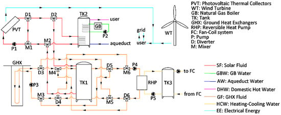
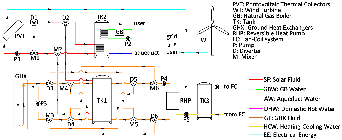
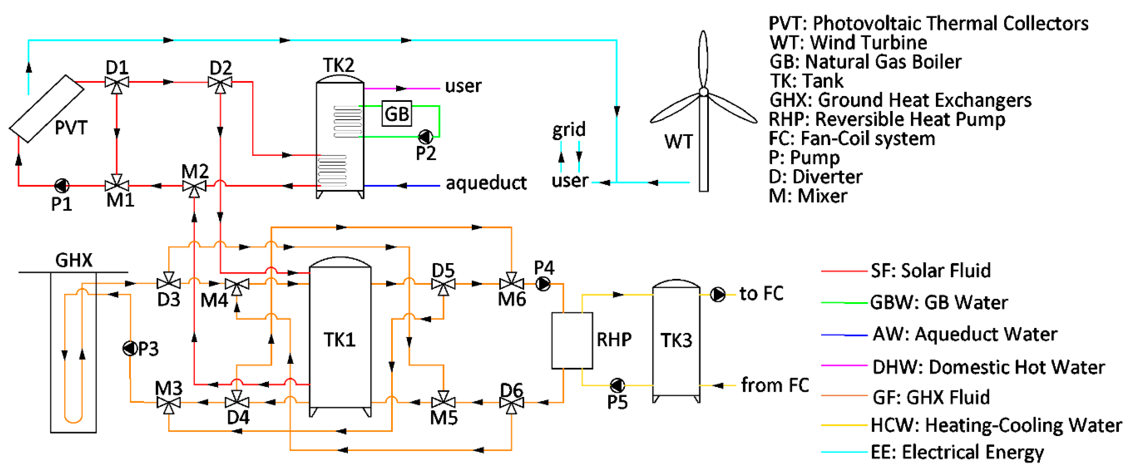
The proposed system includes vertical ground heat exchangers coupled with a reversible heat pump for space heating and cooling purposes, and a photovoltaic/thermal solar collector field assisting the ground heat exchanger in the heating operation during winter and preheating the domestic hot water all year long. The solar field and the micro wind turbine are used for the generation of electrical energy, matching in part the demand of the user.
The basic layout of the system, including all the main components and loops, is shown in
Figure 1.
The loops of the system were designed to manage adequately the thermal energy flows in order to match the thermal energy demand of the user. The loops consist of:
- -
solar fluid (SF) consisting of a 40% propylene glycol-water mixture used to cool the photovoltaic/thermal collector and supply thermal energy to assist the heating of the ground heat exchanger tank and to preheat the domestic hot water;
- -
ground heat exchanger fluid (GF) consisting of the same glycol-water mixture of SF and used to extract or dissipate the heat form or to ground, store the thermal energy and supply the source side of the water-to-water heat pump;
- -
heating and cooling water (HCW) used as working fluid at the load side of the heat pump and supplied to the user fan-coil system;
- -
gas boiler water (GBW) used to transfer the heat from the natural gas boiler to the domestic hot water tank;
- -
Aqueduct water (AW), fresh water used for sanitary purposes;
- -
domestic hot water (DHW), water heated by the solar energy and natural gas boiler operation supplied to the user;
- -
electrical energy (EE) produced by the photovoltaic cells and wind turbine in order to match a part of the user demand.
The devices that were integrated in the system layout are the following:
- -
ground heat exchangers (GHX) consisting of 2 vertical U-tube shape polyethylene heat exchanges arranged in parallel, used to extract and dissipate the thermal energy during the winter and summer operation of the heat pump;
- -
photovoltaic/thermal collectors (PVT) consisting of one glazed flat plate units integrating monocrystalline photovoltaic cells;
- -
wind turbine (WT), a micro-scale wind turbine
- -
reversible heat pump (RHP), a water-to-water unit single-stage unit allowing to modulate the thermal power;
- -
thermal storage tank (TK1), consisting of a thermally stratified unit allowing to store the thermal energy produced by GHX and PVT during winter used to supply RHP, and to buffer the heat rejected by the heat pump during summer before the dissipation by GHX;
- -
domestic hot water tank (TK2), consisting of a tank with two internal heat exchangers used to heat the water by the solar loop (HX1) and by the natural gas boiler (HX2);
- -
natural gas boiler (GB) used as an auxiliary device producing DHW by means of TK2 in case of scarce availability of solar energy;
- -
hydronic system buffer tank (TK3), consisting of a double inlet-output storage used as inertial tank for fan-coil the heating and cooling system;
- -
fan-coil system (FC), consisting a water to air units providing space heating and cooling for the rooms of the building, supplied by heated or cooled water produced by RHP.
The system layout included also several devices in order to manage properly the fluid loops, as diverters (D), mixers (M), and single (P2, P3, P4, and P5) and variable speed (P1) pumps. It is worth noting that the layout presented in
Figure 1, is a simplified version of the system implemented in the simulation environment, since this one includes also other components, like controllers, weather database and components generating the results of the simulation as plotters, variable integrators and printers. The controller components were coupled together in order to develop an efficient control strategy of the system, described as follows.
In the heating season, the ground heat exchanger heated the working fluid provided by the bottom of the storage tank. The heated fluid was supplied to TK1 by means of a stratification supply system that allows one to supply the fluid to the tank to the node with the temperature closest to the entering fluid. In this way, the fluid with a higher temperature was supplied to the top part of the tank while the fluid with a lower temperature was supplied to the bottom part, ensuring thermal stratification of the storage. From top of TK1, the mixture of glycol and water was supplied to the source side of the reversible heat pump, which operated in order to keep the temperature of the buffer tank TK3 within a fixed dead band. RHP was activated when the temperature inside the tank drops to 35 °C while it was turned off when the temperature increased to 38 °C, in order to avoid an unnecessarily heating of TK2. Moreover, during the heating operation, the heating power of RHP was modulated by means of a proportional controller as a function of the tank temperature. The control strategy was developed to set the power of RHP to 100% when a temperature of 35 °C inside the TK3 tank was reached, while it was set to 20% for a temperature of 37 °C. It is worth noting that the activation of the pump dedicated to GHX was activated only when RHP was turned on in order to avoid an unnecessarily electrical energy consumption, and this control strategy was performed during both heating and cooling periods.
RHP ensured a proper operation of TK3 in terms of temperature required by the fan-coil system for the space heating, with the last one activated in order to ensure a temperature of the air inside the building rooms between 20 and 22 °C.
During the cooling season, the RHP was activated in a chilling mode in order the keep the TK3 temperature between 10 and 7 °C, and similarly in the winter period the unit cooling power was modulated proportionally the TK3 temperature. In fact, the load factor of RHP was set to 100% when a temperature of 10 °C inside the TK3 tank was reached, while it was set to 20% for a temperature of 8 °C. During the operation of RHP in cooling mode, the heat rejected by the condenser of the unit was supplied by means of GF to the top of TK1, and from there was dissipated by GHX.
The operation of the loops at the load and source side of TK1 were managed by a diverter and mixing valve system, consisting of D3–D6 diverters and M3–M6 mixers. In particular, the valves were used to supply GHX with the fluid stored in the bottom part of TK1 (lowest temperature) and to supply RHP with the fluid stored in the top part of TK1 (highest temperature) during winter. The same system was used in summer in order to supply from the bottom part of TK1 tank the fluid entering the condenser of RHP and to supply GHX with the fluid stored in the top part. The adoption of this valve system allowed one to operate both GHX and RHP with in a proper way from the level of temperature point of view.
The photovoltaic/thermal collectors were used all year long to heat the water stored in the bottom part of TK3, in order to produce DHW, while during winter they were used also to heat TK1 aiding the space heating operation performed by RHP. The pump of the solar collectors was activated when the solar radiation increases above 100 W/m2 in order to avoid a possible cooling of the fluid flowing within the collectors. Moreover, in order to avoid a possible cooling of TK1, during winter, and TK2, all year long, a by-pass consisting of D1 and M1 valves was adopted. On the basis of which the tank was supplied by solar collector, the control strategy checked continuously that the fluid temperature exiting the collectors was at least 2 °C higher than the one inside the tanks before supplying it to the storage. If such a condition was not met, SF was recirculated within the collectors and M1 and D1 valves. In detail, in this control strategy, the solar collectors’ outlet temperature was compared to the top temperature of TK1 and to the water temperature inside TK2 at the level of the internal heat exchanger supplied by the solar loop. The setpoint temperature of the solar collectors was set by means of the operation of the variable speed pump and depended on the tank to be loaded: 30 °C for TK1 and 60 °C for TK2.
The heating operation of TK2 by the solar system was set to be performed until the water near the bottom internal heat exchanger of the tank reached the setpoint value of 55 °C. In case the DHW demand is not met by solar thermal energy, GB is activated. In particular, then the TK2 top temperature drops to 50 °C GB is turned on in order to heat the water up to 55 °C. The auxiliary operation of GB allows one to match the user DHW independently from the availability of solar energy.
The solar loop operation during winter was designed to heat primarily TK3 and secondarily TK1. The heating of TK1 was allowed only when the temperature of the fluid exiting the solar collectors was not enough high to heat the water near the lower internal exchanger of TK2 (SF temperature 2 °C higher than that of the water). Once the temperature of the fluid exiting PVT increases above the threshold relative to the temperature of TK2, the heating of the DHW is allowed.
Finally, the electrical energy produced by the PVT and WT is supplied to the user or to the grid depending on the demand. The grid allows one to store virtually the energy produced in excess and use it part when the demand overcomes the production.
2.2. Ground Heat Exchanger
The component has been implemented using the Type557 model, simulating a vertical heat exchanger that transfers heat with the ground. The adopted model allowed one to simulate both U-tube ground heat exchanger or a concentric tube ground heat exchanger by means of a subroutine. Nevertheless, for the purposes of this study, the U-tube sub-model was adopted.
The component simulated both heating and cooling operation of the heat exchanger, since the working fluid may absorb heat from or reject it to the ground as a function of the temperatures of the fluid and the ground surrounding the heat exchanger.
The adopted model was based on the following assumptions:
- -
uniform placement of the boreholes within a cylindrical storage volume of ground;
- -
conductive heat transfer between the heat exchanger and the storage volume, and convective heat transfer between the fluid and the pipes;
- -
adoption of global temperature, local solution, and steady-flux solution methods for the calculation of the ground temperature, where an explicit finite difference method was used for the global and local problems, while an analytical approach was used for the calculation of the steady flux solution. The approaches were coupled together by means of a superposition method in order to calculate the temperature within the ground storage.
The detailed description of the model is here omitted fake of brevity. Its comprehensive presentation is available in reference [
33].
2.3. Phototoltaic/Thermal Collectors
The solar field is equipped with flat-plate photovoltaic/thermal solar collectors, consisting of a conventional solar thermal device with an absorber covered by a PV cell layer encapsulated within a transparent protective layer, typical of PV panels. The model of the PVT collector was based on the flat-plate thermal collector mathematical model modified in order to take into account the presence of the PV cell panel. In detail, the TRNSYS model Type50 was used for the simulation of the solar field, where constant values for the overall energy loss coefficient, the glass transmittance, and the absorbance of the absorber were assumed. The model was based on several equations, and the most important ones have been presented below.
The modified Hottel–Willier–Bliss method [
34] and an energy balance was adopted in order to calculate the PV cell temperature (
Tcell). The overall thermal loss coefficient of the collector per unit area (
Ul*), overall collector heat removal efficiency factor (
FR) and the PVT thermal power output (
QPVT) were calculated with the following equations:
where
Itot is the solar radiation,
τg is the glass transmission coefficient,
fp is the efficiency factor,
mf is the mass flow rate,
cf is the fluid specific heat,
APVT is the area of PVT,
αPVT is the PVT absorption coefficient
Tf,in is the fluid inlet temperature and
Tamb is the ambient temperature. The PVT electrical efficiency (
ηPVT) was calculated on the basis of the temperature of the photovoltaic cell:
where
ηPVT,ref is the reference PVT electrical efficiency,
βPVT is the efficiency temperature coefficient,
Tcell is the photovoltaic cell temperature and
Tref is the reference temperature. In addition, energy balances of the collector were used to calculate the electric power and the outlet temperature of the fluid.
2.4. Wind Turbine
The built-in library TRNSYS component Type90 was used to simulate the micro-wind turbine. The adopted model calculated the power produced (
PWT) as a function of air density (
ρ), power coefficient (
cp), rotor area (
Ar) and wind speed (
v), as follows:
where
cp is dependent on the axial induction factor (
a) according to the following equation:
When
a reaches the value of 1/3,
cp reaches the maximum theoretical value of 0.593, according to the Betz limit [
35].
The effect of the variation of the height above the ground of the site of WT installation was taken into account by the model in terms of the air density variation and the increase of wind speed. The density of air as a function of the height (
z) was calculated with the ideal gas law where temperature (
Tz) and pressure (
pz) are considered:
Tz is determined on the basis of the vertical gradient of temperature (“lapse rate” [
36]), as follows:
where
T0 was assumed constant to 15 °C and
B was equal to 6.5 °C/km [
37] Moreover, the pressure
pz was calculated as follows:
where the reference pressure (
p0) is provided on the basis of dynamic local conditions. The wind speed (
v) variation with the elevation was evaluated on the basis of Von Karman analysis [
38]:
where
α is the wind shear exponent, dependent on the site location and its dynamic conditions like atmospheric conditions, presence of objects obstructing the airflow, roughness of the ground surface, etc. In this study, the shear exponent was fixed to 0.14, a value that characterized ideal boundary layer conditions. During the simulation, Equation (10) was used to calculate the wind speed at a certain elevation taking into account time-dependent wind velocities provided at ground level by the Meteonorm weather database included in TRNSYS.
Besides the mathematical formulation of the model, the component in order to calculate the power produced by WT required an external file, where the geometry of the wind turbine as well as the characteristic curve of power as a function of the wind speed were provided. In order to implement such manufacturer data, the data from the datasheet of an ENAIR 30PRO unit [
39] were considered. In order to scale the wind-power characteristic, the manufacturer data was normalized with respect to the nominal power.
2.5. Energy and Economic Model
In order to assess the global energy and economic performance of the hybrid system (HS), a comparison was performed assuming a conventional system (CS) accordingly to the methodology reported in reference [
27,
28]. This approach was adopted since without the adoption of a reference, the energy and economic performance of the hybrid could only have been evaluated in absolute terms, with are not exhaustive for a comprehensive analysis of the system. Using this approach, it was assumed that both HS and CS must supply the same amount of final energy to the user, in terms of space heating and cooling, domestic hot water and electrical energy.
In detail, the reference system consists of:
- -
a natural gas boiler for the production of heat for DHW and space heating, with a seasonal efficiency (
ηGB,ref) of 0.85 [
40];
- -
an electrical chiller providing space cooling, with a seasonal coefficient of performance (
COPcool,ref) of 3.0 [
41];
- -
the electric grid providing electrical energy, with a primary energy efficiency (
ηel,ref) of 0.33 [
40].
HS energy performance was evaluated on the basis of a primary energy (
PE) consumption comparison on a yearly basis with respect to CS.
PE consumption of CS was calculated as follows:
where
Eth,heating and
Eth,cooling was the yearly thermal energy provided for space heating and cooling, respectively, and
Eel,user was the yearly electrical energy demand of the user.
The equation used to calculate the
PE consumption of HS was:
where
EthGB,DHW is the auxiliary thermal energy supplied by GB for the production of DHW and
Eel,grid,net is the energy electrical energy provided by the grid, excluding the electrical energy supplied to and recovered from the grid (net metering) and the
Eel,unrecovered,grid is the electrical energy supplied to the grid and not recovered by the user. On the basis of primary energy consumption, the primary energy saving ratio (
PESr) was evaluated as follows:
The economic performance of HS was evaluated taking into account its investment costs and the operating costs of both HS and CS. In particular, the literature and market cost data were used to determine the capital cost of proposed system components, in accordance with the procedure adopted in reference [
28]. In particular, the following cost function were adopted:
where
LGHX is the length of the vertical ground heat exchangers,
APVT is the area of the PVT collector field,
PWT is the nominal power of WT,
Qnom,heat,RHP is the nominal thermal power of RHP and
VTK1 is the volume of TK1. It is worth noting that the costs of the other tanks (TK2 and TK3) were not taken into account since the devices were assumed to be already present in CS.
The total cost of HS was evaluated summing the cost evaluated by Equations (13)–(17) and adding 10% in order to take into account for the balance of plant components like valves, pumps, etc.
The operation costs for both HS and CS were calculated assuming constant electrical energy tariff (
cel) of 0.133 €/kWh and natural gas price (
CNG) of 0.50 €/m
3 characterized by a reference low heating value (
LHVNG) of 9.59 kWh/m
3 [
40,
42].
For HS, a net metering system, thus the possibility to store and utilize on demand the electrical energy produced in excess, was implemented by means of a bidirectional connection with the grid. In particular, it is assumed that in case of a system with nominal power up to 10 kW it is possible to recover freely up to 80% of the energy supplied to the grid, while the eventual quote exceeding 80% is paid with a mean price for electrical energy. In the case of a nominal power between 10 and 40 kW, the limit is lowered to 70%. This net metering method is adopted in Poland in order to increase the share of small-scale renewable systems in the electrical energy market [
43].
Therefore, the operation cost of HS (
Cop,HS) and CS (
Cop,CS) and the savings (Δ
Cop,HS) were calculated as follows:
where
Eel,recovered,grid was the electrical energy produced by the system and recovered from the grid above the limit established by the net metering prosumer contract (70 or 80% of the energy sent to the grid)
Finally, the simple pay back (SPB) index was introduced in the economic model in order to evaluate in a simple way the performance of the system in terms of profitability.
3. Case Study
The proposed system was investigated under a case study consisting of a single-family household with a ground floor, an attic and a sloped roof. This building as case study was used in a previous paper of the authors [
28]. However, here it was adopted under different climatic conditions from those used in the previous paper, and with a dynamic electrical energy demand of the user and the simulation of the heating load. The building structure is reported in
Figure 2.
The ground floor area was 100 m
2 with a floor height of 2.70 m, while the attic had the same height as the ground floor and a useful floor area of 75 m
2. The roof slope was 30°. The ground floor consisted of two rooms with an area of 25 m
2 and a room of 50 m
2. The components of the building envelope, like walls, roof, and floor, were implemented assuming several series of layers with a global transmittance reported in
Table 2. The detailed structure of the envelope elements has not been reported here for reasons of brevity.
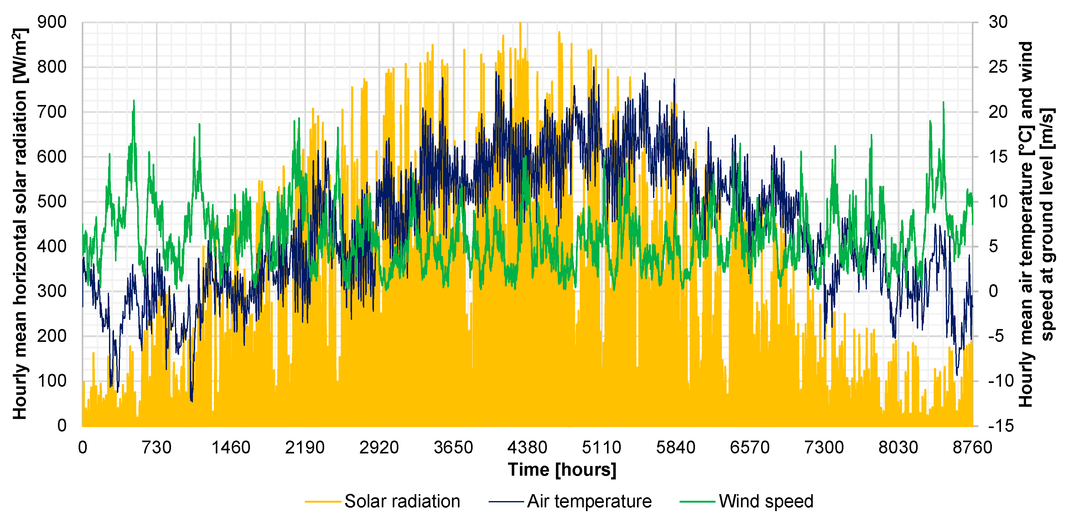
The climatic conditions of Gdansk, Northern Poland, were selected in order to simulate both the system and building operation. For this purpose, the Meteonorm weather database was used, implementing in the simulation a TMY2 file where the mean yearly weather conditions determined on the basis of a 10-year long period were stored. The mean hourly air temperature, horizontal solar radiation, and wind speed at ground level are shown in
Figure 3.
The air-conditioning system of the building integrates an independent fan coil unit for each zone of the house providing space heating and cooling. The space heating period was set from 15 November to 31 March, and the cooling one from 1 May to 15 October. The heating operation was allowed 24 h per day in order to keep the room temperature between 20 and 22 °C, while space cooling was performed between 8:00 am to 10:00 pm in order to maintain the air temperature between 24 and 26 °C.
The model of the building was completed by adding typical loads of a residential house, in order to simulate reliable thermal gains and losses. In particular, the following loads were considered: human activity (5 house inhabitants—sensible heat 75 W, latent heat 75 W), equipment (3.3 W/m2), lights (5.0 W/m2), fresh air infiltration (0.25 Vol/h). In addition, a dynamic DHW demand profile was implemented assuming that each person consumes 60 dm3 of hot water consumption a day.
The electrical energy demand of the user was normalized with respect to the daily demand, and it is reported in
Figure 4 for different days and periods of the year. The profiles were implemented for different days, workdays, Saturdays, Sundays/Holidays, for two periods in the year, period 1 and period 2 assumed from November to March and from April to October, respectively. In particular, the profiles were developed on the basis of standard electrical energy consumption data available for users as the one here investigated [
45] performing a normalization of the hourly data on the basis of daily energy consumption (sum of the hourly consumption). Therefore, the profiles developed were characterized by an integral over 24 h equal to 1.0, thus, in this way it was possible to scale the normalized profiles in order to achieve a fixed annual electrical energy consumption for the user. The yearly electrical energy consumption of the building was set to 5.0 MWh, according to common energy demand levels for this kind of utility [
45].
The main design and operating parameters of the proposed system components are reported in
Table 3. Such parameters were selected on the basis of manufacturer data in order to allows the system a proper operation in terms of the capability of energy transfer, number of activation-deactivation cycles of the components, and to match the user thermal demand.
4. Results and Discussion
The dynamic simulation of the system was carried out for a one-year basis, from 0 to 8760 h. with a 0.04 h time step, calculating temperature and power trends and integrated variables. Under these simulation parameters, a large amount of dynamic data was generated by the simulation, thus for reasons of brevity, only the most important results were reported in this paper. In detail, the dynamic operation of the system is shown for a typical winter operation day in terms of temperature and power trends, while the behavior of the system over the yearly operation was presented on monthly basis. Finally, the yearly results are presented showing the global energy and economic performance. The system is also investigated changing the area of the PVT collector and the nominal power of the wind turbine, remaining the other parameters unchanged. In fact, the dimensioning of the ground heat pump system was performed on the basis of space heating and cooling demand of the user, which is constant under the adopted assumptions.
4.1. Daily Operation of the System in Winter
The dynamic operation of the system was analyzed for all the days of year, nonetheless due to the high amount of data this analysis cannot be presented here; thus, only the results for a winter operation day have been reported. The selected day was 18 February, falling between 1176th and 1200th hour of the year, which presented the full operation characteristic of the system operation from the point of view devices activation.
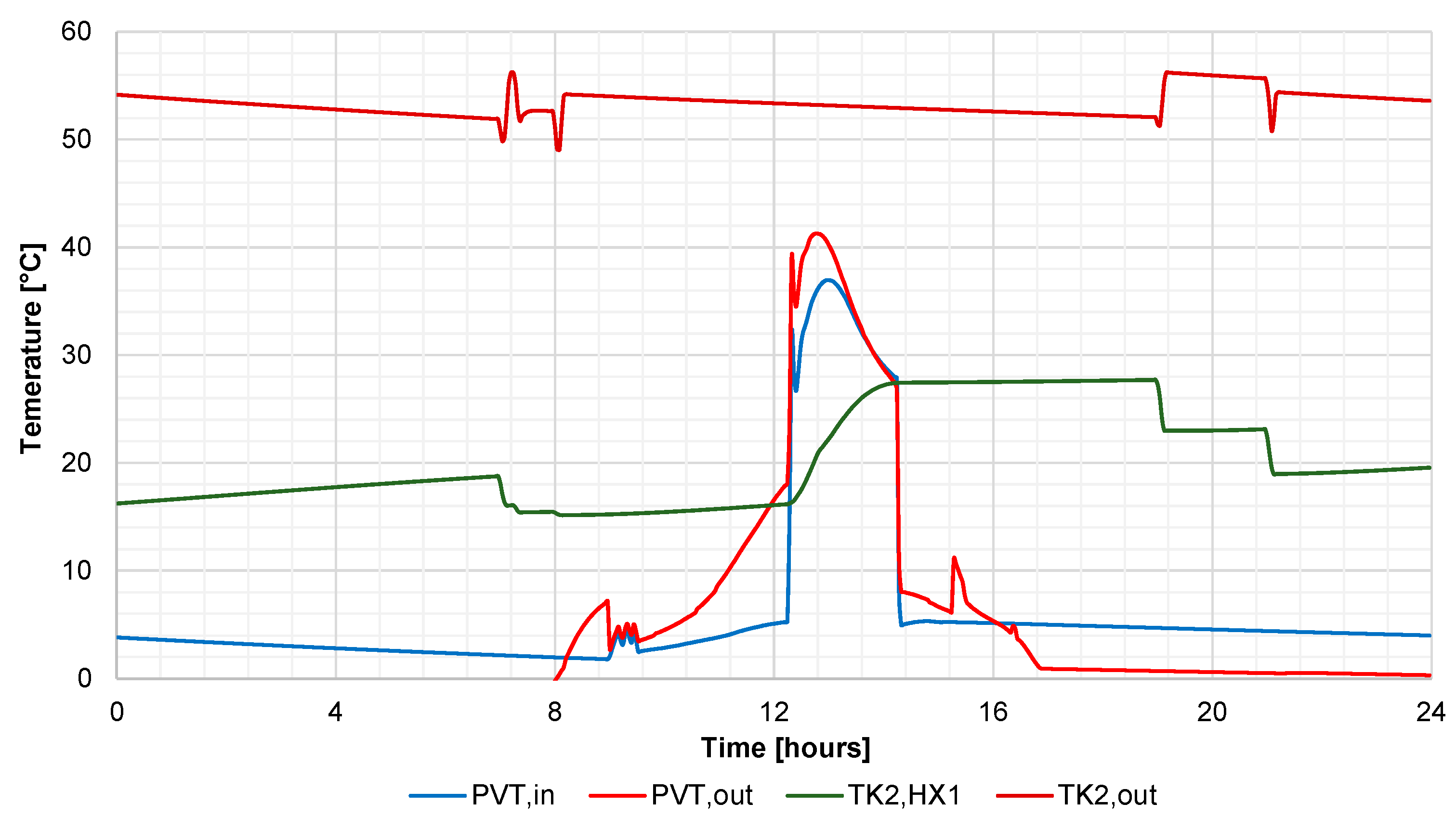
The most important temperatures of the system have been shown in
Figure 5 and
Figure 6. During the firsts hours of the day, both inlet and outlet temperature of GHX (GHX, in and GHX, out) slowly decreases because the heat pump is in operation and this determines a decrease of the temperature at the bottom of TK1, which supplies GHX. The decrease is also due to the fact that thermal energy produced by the PVT during the previous day slightly increased the temperature of the GHX loop. From 0:00 am to about 8:00 am the heat pump is supplied with GF at a temperature about 3 °C (TK1, out), while the temperature exiting the evaporator of RHP (RHP, source, out) oscillates slightly above 0 °C, due to the supplied heat to run the heat pump. After 8:00 am, PVT solar collectors start to supply heat to TK1 and the heat pump starts to reduce the heat output, determining an increase of its top temperature and as a consequence an increase of the temperatures in the GHX-RHP loop. The temperature at the outlet reaches a temperature of about 9 °C just after 12:00 am, and after then starts to decrease because TK2 starts to be heated with solar thermal energy. However, when this operation stops, the heating of TK1 is again performed but the temperature keeps to decreasing due to the operation of RHP.
It is worth noting that during the central hours of the day the temperature at the outlet temperature of RHP condenser slightly decreases while the heated water (HCW) at the outlet of TK3 (TK3, out) increases. This situation is achieved since the heat pump thermal output decreases as a function of a reduction of the space heating load of the building.
As concerns the PVT and TK2 loos, the results point out a decrease of the inlet temperature of PVT (PVT, in) in the night hours due to the heat losses on the pipes connected to the solar field. At the same time, the water temperature at the top of TK2 (TK2, out) decreases being the heat transferred to the lower parts of the tank where the temperature is slightly lower. In fact, the temperature of the water inside the tank near the solar heat exchanger (TK2, HX1) increases during the night by about 2 °C. After 8:00, am the temperature at the outlet of PVT collectors (PVT, out) increases above the inlet one allowing to start the heating of TK1. However, this operation is performed only when the outlet temperature is 2 °C higher than the top of TK1, according to the developed control strategy. The TK1 heating operation ends after 12:00 am when the PVT outlet temperature overcomes by 2 °C the temperature of the water inside TK2 near HX1, which is the condition that triggers the heating of TK2. The control system sets the PVT setpoint temperature to 60 °C from the previous value of 30 °C, thus the outlet temperature increases due to the reduction of the mass flow rate of SF operated by P1 and the proportional controller. In the result, the solar heat increases the water temperature at the bottom of TK2 to about 28 °C, allowing the preheating of DHW, and this temperature level is maintained until occurs the next DHW request near 7:00 pm. During the selected day the heating operation of DHW is completed by GB, which maintains the temperature at the top of TK2 (TK2, out) between 48 and 55 °C.
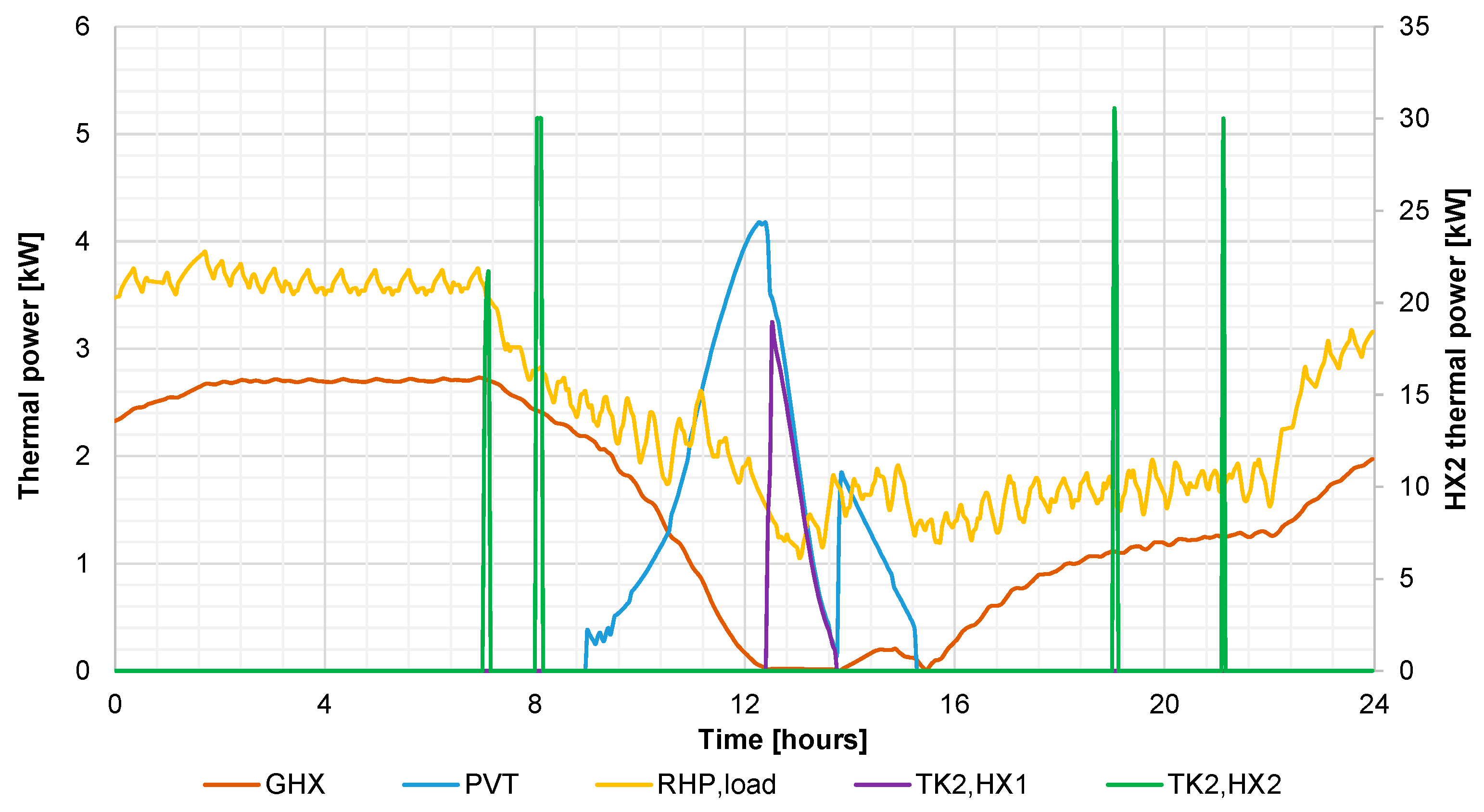
The thermal and electrical powers for the selected day are reported in
Figure 7 and
Figure 8, respectively. The thermal power of the ground heat exchanger (GHX) varies as a function of the temperature of the tank (see
Figure 5) and the thermal power supplied by the heat pump to the user (RHP, load). The thermal demand for space heating is higher, and the heat extracted from the ground is higher. During the day, the reduction of the heating demand along with the heating of TK1 by the solar field implies a decrease of the thermal extracted by GHX to zero just after 12:00 am, since the increase of the temperature of the working fluid of GHX is not possible due to the thermal conditions of the ground coupled with a relatively high bottom temperature of TK1. The solar field thermal power (PVT) increases up to 4 kW at noon, then the heat starts to be transferred to TK2 with lower power (TK2, HX1). This is due to a higher water temperature inside TK2 with respect to that present at the bottom of TK1, which limits the solar heat transfer rate to the tank. The heating of TK2 by renewable thermal energy is not adequate to match the DHW demand, thus the activation of the GB and the heating of the top part of TK2 by HX2 is mandatory (TK2, HX2).
The electrical power trends highlight that during the night hours the output produced by the wind turbine (WT) is lower than the total power demand of the user, consisting of the building equipment, heat pump, and system auxiliaries operation. Therefore, a significant part (about 1/3) of the user demand (user) must be matched by the energy supplied by the grid. This mainly consists of the grid energy that is not taken into account by the net-metering system (net grid) since the contribution of the energy recovered by the grid (from the grid) is marginal. Only for about the first hour of the day, the user demand is matched by the energy that was produced during the previous day and supplied to the grid.
The system operates in the central hour of the day denotes that a certain amount of energy produced by the system is supplied to the grid (to grid), due to the output of the PVT field. The energy virtually stored by the grid is immediately supplied again to the user once the power generated by the system (PVT + WT) decreases below the demand just before 3:00 pm.
4.2. Monthly Results
The results were analysed by performing an integration of the powers on a monthly basis, thus the oscillations typical of the dynamic system operation were agglomerated in the integral results. The main thermal energy flows in the system are shown in
Figure 9. Here, the effect of the user space conditioning demand on the system behavior is clearly shown, since the thermal energies flows inside the system are significantly higher during the winter heating season compared to the cooling one.
The energy extracted by the ground heat exchanger (GHX) rages between 0.78 MWh to 1.41 MWh assuming a trend dependent on the thermal energy supplied by the load side of RHP (RHP, load). It is worth noting that as expected the major part of the thermal demand of the RHP evaporator is provided by GHX (at least 75.3% for all the months), while a relatively small part is provided by PVT (between 6.5% and 26.5%). From the point of view of summer operation, the heat rejected by GHX is from 11 to 37% higher than the one transferred by the condenser of the heat pump (RHP, source), and this is due to the fact that the pump of GHX (P3) operates independently from that of RHP (P4).
Moreover, it is important to note that the monthly thermal energy produced by PVT (PVT) outside the heating season is relatively small compared to the solar energy available (solar). This occurs because the solar field area is oversized with respect to DHW demand present during summer, and this determines a decrease in the thermal performance of the solar collector.
The monthly electrical energy flows are shown in
Figure 10. The solar field electrical energy production (PVT) following the trend of the solar energy availability reported in
Figure 9 ranges between 0.048 and 0.30 MWh. The energy production of the PVT field is lower than the one achieved for the wind turbine (WT) during winter, while the opposite occurs during summer. In particular, the system receives from WT between 0.11 and 0.40 MWh of electrical energy which is used to match in part the user demand.
The results also point out that the operation of the heat pump for space heating significantly affects the user’s electrical energy demand during winter, since in summer the thermal energy removed by RHP from the user in the form of space cooling is relatively small, as outlined in
Figure 9. Under these conditions, the production of electrical energy during the year by both PVT and WT determines the that during winter the amount of energy withdrawn from the grid excluding the net-metering (net grid) is relatively high, being between 41.1% and 58.8% of the demand (user). Conversely, it is null during the summer due to favorable conditions of demand and energy production. In addition to this, it noticeable that the energy produced in excess by the system (to grid) is always above zero, and increases significantly during the central months of the year, as well as the energy recovered from the grid in the frame of the net-metering contract. However, is it interesting to observe that the electrical energy stored virtually in the grid during April and May can be recovered in October and November when the PVT energy production drops.
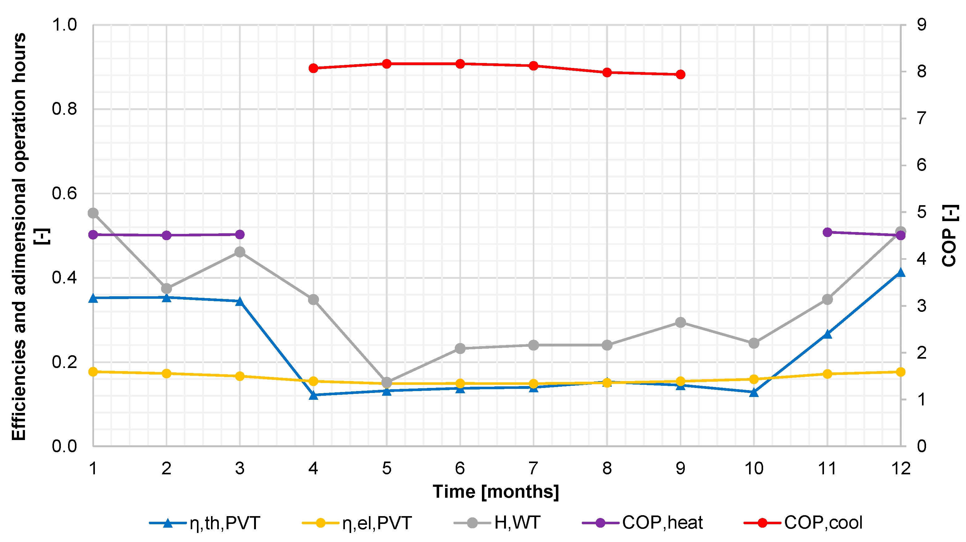
The main efficiency parameters of the hybrid system are reported in
Figure 11. As preliminarily mentioned, the thermal efficiency of the PVT field (
η, th, PVT) in winter is relatively higher than the one achieved in summer, since the temperature of the solar loop increases when only DHW is produced. In fact, the aperture area of the collector allows one to match the major part of the DHW demand in the summer months (more than 70% of the demand). It is worth noting that it is not possible to achieve a higher value due to the time of the DHW demand, occurring in the morning and late evening hours when the solar energy availability is relatively lower.
The decrease of the PVT thermal performance also negatively affects the electrical efficiency (
η, el, PVT), being the PV cell affected by the operation temperature of the solar collectors. The efficiency decreases of about 15.9% with respect to the maximum value of 0.177 achieved in January and December. The wind turbine performance is presented in
Figure 11 as a function of the normalized equivalent number of operation hours (H, WT) defined as the ratio between the equivalent hours of the wind turbine and the total number of hours in the considered time interval. As expected, the performance of WT decreases in summer, operating in terms of equivalent hours less than 30% of the time due to a lower availability of the wind energy source characteristic of the selected location.
Finally, the performance of the heat pump in terms of COP for space heating (COP, heat) and cooling (COP, cool) highlights that the device operates under stable conditions in terms of source and load temperatures. The COP in winter varies less than 1.5% compared to the maximum value of 4.57, while during summer the variation is 2.8% with respect to the maximum value of 8.17.
4.3. Global Energy and Economic Results
As done for the monthly analysis, the yearly results are analysed performing the integration of the variables from 0 to 8760 h. The main thermal and electrical energies of the system in the yearly time scale are reported in
Table 4. Analysis of the results shows that despite a significant availability of solar energy (
Esol,PVT) the production of thermal energy by the PVT field (
Eth,PVT) is less more than 50% of the thermal energy produced by GHX in total (
Eth,GHX,heat and
Eth,GHX,cool). As shown by the monthly analysis, the ground heat exchanger is significantly more exploited in winter compared to summer due to different space conditioning demands, as outlined by the fact that the winter energy extracted 6.4 times higher than the heat rejected in summer.
It is interesting to note that the yearly DHW demand (Eth,DHW) is matched by solar energy only in 38.7%, and this occurs because the contribution of the solar energy to the production of DHW (Eth,HX1) during winter is almost null, while during summer it not exceeds 75.3%.
From the point of view of electrical energies, among the generation devices, WT produces more energy. In fact, the yield of PVT (Eel,PVT) is 0.87 MWh less than the one achieved by WT (Eel,WT), due to the comparatively better availability of wind energy compared to the solar one for the selected locality. The results also show that the incidence of the system auxiliary devices (Eel,AUX) on the system electrical energy balance is negligible, the energy demand of such equipment being only 5.6% of the total amount (Eel,demand), while the yearly energy demand of the heat pump is significant, since its operation determines 25.4% of the annual energy bill.
Moreover, the analysis of the energy flows among the system and the grid points out that the electrical energy supplied to the grid (Eel,to grid) and recovered (Eel,from grid) is the same, and thus the full bidirectional net-metering balance is achieved. In particular, the user sends to the grid 24.5% of the electrical energy produced, while the grid supplies the user with net-metering-free energy (Eel,net grid) in order to cover the demand in 31.4%.
The energy and economic indexes of the system are presented in
Table 5. The savings of HS in terms of primary energy with respect to CS (
PESr) are remarkable (66.6%), nonetheless, some primary energy must be consumed by HS due to the grid intervention to meet the electrical energy demand and to the operation of GB, especially during winter.
The scarce thermal efficiency of the PVT field affects the total efficiency of the collector units (33.1%), while the wind conditions of the selected locality allows one to achieve a good performance of WT, the normalized number of equivalent operation hour being equal to 0.333. This value underlines that the amount of electrical energy produced by WT is one-third of the maximum achievable for such a unit under ideal operational wind conditions (wind speed always above 11 m/s).
The yearly performance of the heat pump for heating and cooling overcomes the nominal conditions, indeed both COPs are higher than the values reported in
Table 3. Such a result is achieved because: (i) during the winter the operation of GHX and PVT allows the evaporator of RHW to operate at a relatively higher temperature, and the outlet condenser temperature is lower than the nominal one (45 °C), (ii) in summer GHX allows one decrease the condenser temperature below the nominal operation conditions (30 °C).
On the basis of the comparison in terms of operational cost between CS and HS, the proposed innovative system allows one to save 0.900 k€/year which is 65.4% of the operational cost of the conventional system. Nevertheless, taking into account the fact that the investment for the whole hybrid system is relatively high (almost 20 k€), the economic performance of the investigated solution is scare. SPB is slightly over 21 years, which implies a feasibility of the system outside reliable criteria for economic investments. However, assuming that both PVT and WT are financed by 70% from incentive policies, SPB value decreases to 11.6 years, which is a value that starts to be economically viable. It is worth noting, that such incentive strategies, based on capital incentives, are increasingly common across Europe, and thus its applicability is reasonable. Moreover, it is worth noting that the proposed economic analysis of the system is performed under the worst scenario, where that total cost of the investment is considered. In case of the necessity of the installation of a new system providing DHW, heating and cooling, or in case of the substitution of the existing one, the cost that should be considered in the investigation would be only the difference of cost between CS and HS. Under such conditions the profitability of the system would be better compared to the present analysis. An interesting possibility of incentive for the proposed system could be that based on the consumption of produced renewable thermal and electrical energy, thus an additional saving may be generated by the hybrid system. In the invested case study, if an incentive of 0.05 €/kWh is adopted for both thermal (heating and cooling) and electrical energy produced and consumed by the user, SBP decreases to 13.1 years.
4.4. Parametric Analysis
The energy and economic performance of the system was also investigated changing the extension of the PVT field and the nominal power of WT. This analysis was performed with the aim of determining the effect of such design parameters on the global results when all the other ones are assumed to be constant. The PVT area was varied from 3.0 to 15.0 m2, with a step to 3 m2, whereas WT power was increased from 0.3 to 1.5 kW, with a step of 0.3 kW.
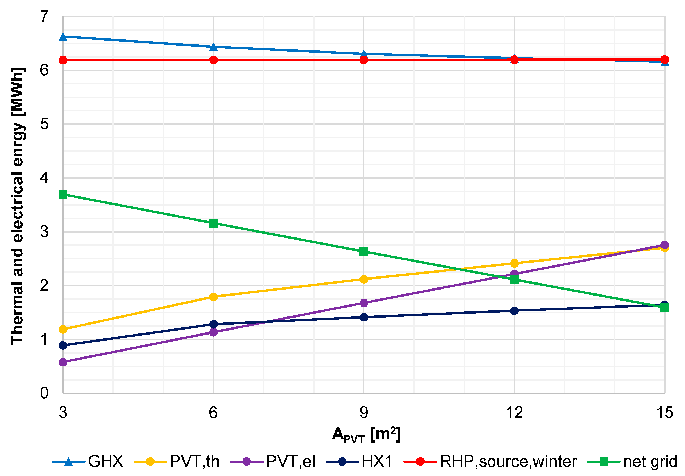
The results of the parametric analysis as a function of the PVT field area is presented from the point of view of energy in
Figure 12, and from that of the efficiency and economical viewpoint in
Figure 13.
The variation of PVT area affects almost linearly the electrical energy producible by the solar field, thus the negative effect of a mean higher solar loop temperature achievable for a higher collector extension is limited. As a consequence, the electrical energy supplied by the grid and the net of the net-metering contract decreases linearly. The opposite occurs for the thermal energy produced by PVT collectors, increasing less when the area is gradually augmented. In particular, the increase of the thermal energy produced by the field configuration of 3 to 6 m2 is 0.606 MWh, whereas from 12 to 15 m2 it is only 0.288 MWh. The increase of the production of the thermal energy by PVT implies a decrease of the thermal energy extracted by GHX, due to a higher mean temperature of TK1, and an increase of the heat supplied to TK2 by means of HX1. Nevertheless, the yield of GHX is scarcely affected by such variation, because the additional thermal input of the PVT field to TK1 achieved in case of a higher area is marginal, and a similar situation is achieved for HX1. In this case, the solar field reaches the almost the maximum capability of providing heat to TK2, due to the DHW demand and dynamics of solar thermal energy production during the day, for and PVT area above 6 m2. Additionally, it can be observed that the increase of the collector area does not affect the thermal energy used by the load side of RHP (evaporator) to match the used space heating demand, the latter being constant. In addition to this, also the COP of RHP in heating model remains practically constant, showing that the contribution of the solar field to the heating of TK1 is negligible.
The thermal efficiency of PVT decreases more than two times when the area increases from 3 to 15 m2, due to the previously discussed reasons, highlighting that the increase of the PVT field extension significantly affects the operation of the solar system in terms of thermal efficiency. On the other hand, a limited decrease of the electrical efficiency of PVT is achieved along the range of investigated area values (only 5.1%), because the increase electrical losses of PVT due to a higher PV cells temperature is marginal.
The savings of primary energy achievable by HS increase as a function of the PVT area on the basis of a higher thermal and electrical energy produced and used in the system. However, the main reason for the increase of PESr is due to the production of electrical energy rather than the production of heat, being the effect of the last one on the energy balance of the system relatively marginal. Therefore, in terms of primary energy savings, it is convenient to increase the PVT area, and the same condition is achieved from the economic viewpoint, since SPB decreases for a higher area. However, the decrease is not sufficient to achieve the system economic profitability because the value remains over 21 years.
The capacity of WT affects only the electrical energy flows in the system as the thermal and electrical parts of the system are decoupled. The increase of WT nominal power, keeping constant the hub height and the wind conditions, determines a proportional increase of the generated electrical energy, which is equal to 2.92 MWh per kW. In view of this trend, the electrical energy supplied to the grid and withdrawn from the grid increases as well for a larger wind turbine, although the increase, in this case, is not linear due to the characteristic curve of the device. In fact, the increase of power from 0.3 to 0.6 kW implies a variation of energy supplied to the grid of 0.196 MWh, although the increase of 0.544 MWh for the variation from 1.2 to 1.5 kW. Moreover, it is important to note that beyond 1.2 kW of WT power, it is not possible to recover all the electrical energy supplied to the grid, since due to the intrinsic characteristic of the user demand and dynamic production of electrical energy by PVT and WT. Therefore, even when a turbine with a larger diameter is installed, the electrical energy needed from the grid is not null for the WT capacities considered. In practice, the increase of the wind turbine yield per unit of power determines the same reduction of the electrical energy produced within the grid and required by the user is needed to match the demand.
Finally, the analysis of primary energy savings shows that the trend of energy production achieved increasing the WT capacity directly affects PESr, and this is achieved because a higher production of electrical energy means a higher saving of non-renewable energy provided by the grid to the user. In the investigated case, the numerical data shows that increasing WT power 5 times implies an increase of PESr of 82.3% compared to the value achieved for a 0.3 kW unit.
As concerns the economic savings of HS with respect to CS, they increase of 67.0% passing from a wind turbine with 0.3 kW to a one with 1.5 kW, and on the other side in the same range of power, the total cost of the system (C, tot) increases of 30.6%. Therefore, coupling these two economic conditions, it is clear why the trend of SPB is decreasing as a function of WT power. In particular, SPB trend passed from 25.4 years for a 0.3 kW unit to 19.8 years for a power 5 times higher, consequently, the effect of higher savings overcomes the effect of the system cost increase when larger wind turbines are considered.
5. Conclusions
In the paper, a novel micro-scale hybrid geothermal-solar-wind system for a residential user has been investigated through dynamic simulation performed using a complex model developed in TRNSYS software [
26]. The layout of the system included vertical ground heat exchangers, photovoltaic/thermal solar collectors, wind turbine, net-metered bidirectional connection with the grid, and a water-to-water reversible heat pump. The system was used to match a part of the user electrical energy demand, and to provide space heating and cooling along with DHW. The dynamic operation of the system and the building was simulated simultaneously in order to take into account their mutual interaction. In order to investigate the system, a case study of a single-family house under Polish northern climatic conditions, and a conventional reference system for the user, were considered.
The operation of the system was investigated from the viewpoints of temperature and thermal and electrical power trends for a selected winter day. Monthly and yearly analyses were carried out in order to assess the energy and economic system performance during the year and in terms of global performance. The study was concluded performing a parametric analysis of the system, where the solar collector field area and micro wind turbine power were varied.
The main results of the study were the following:
- -
during the firsts hours of winter operation day, both inlet and outlet temperature of the ground heat exchanger slowly decreased due to operation of the heat pump, determining a decrease of the temperature at the bottom of the tank storing the working fluid of the heat exchanger;
- -
the morning hours of a winter day, the hybrid solar collectors start to supply heat to the ground heat exchanger storage tank and the heat pump starts to reduce the heat output, determining an increase of the tank temperature and as a consequence an increase of the temperatures in the loop of the ground heat exchanger and source side of heat pump;
- -
the energy extracted by the ground heat exchanger ranges between 0.78 MWh to 1.41 MWh per winter month assuming a trend dependent on the thermal energy supplied by the load side of the reversible heat pump. The major part of the thermal demand of the heat pump evaporator is provided by the ground (at least 75.3% for all the months), while a relatively small part is provided by the solar field (between 6.5 to 26.5%);
- -
the production of electrical energy along the year and the user demand determine that during winter the amount of energy withdrawn from the grid excluding the net-metering is relatively high, being between 41.1% and 58.8% of the demand. Conversely, it is null during the summer due to favorable conditions of demand and energy production;
- -
the ground heat exchanger is significantly more exploited in winter compared to the summer due to different space conditioning demand, as outlined by the fact that the winter energy extracted was 6.4 times higher than the heat rejected in summer;
- -
the savings of the hybrid in terms of primary energy with respect to the reference system are 66.6%, nonetheless, some primary energy must be consumed by the proposed system due to the grid intervention to meet the electrical energy demand and to the operation of the gas boiler in order to match the domestic hot water demand, especially during winter;
- -
the simple pay back period is slightly over 21 years, implying a scarce economic feasibility of the system. However, assuming that both solar field and wind turbine are financed by 70% from incentive policies, the payback time decreases to 11.6 years;
- -
the increase of the thermal energy produced by the field configuration of 3 to 6 m2 is 0.606 MWh, whereas from 12 to 15 m2 it is only 0.288 MWh. The increase of the production of the thermal energy by the solar field implies a negligible decrease of the thermal energy extracted by the ground heat exchanger, due to a higher mean temperature of the storage tank;
- -
the increase of wind turbine nominal power, assuming constant the hub height and the wind conditions, determines a proportional increase of the generated electrical energy, which is equal to 2.92 MWh per kW.
The present study outlined that the hybrid system under consideration achieves a satisfactory performance in terms of energy, whereas its economic profitability is not adequate to permit its application as a valid alternative compared to an existing reference system based on a natural gas boiler from domestic hot water production and heating, an electrical chiller for space cooling and the grid for matching user demand. However, considering the installation of a new system matching the user demand, or in the case of the substitution of the existing one, only the extra cost for the hybrid system with respect to the reference one must to be considered. Thus, the profitability of the hybrid system will increase and the gap between the reference system in terms of economic competitiveness will be significantly reduced.
The investigations of the proposed system will be expanded by performing analyses regarding the modification of the system layout, comprehensive parametric analysis of the system, and optimizations aiming at determining the characteristics of the system depending on the design parameters and user type and behavior.


