Abstract
The paper presents an analytical mathematical model of a car radiator, which takes into account various heat transfer coefficients (HTCs) on each row of pipes. The air-side HTCs in a specific row of pipes in the first and second passes were calculated using equations for the Nusselt number, which were determined by CFD simulation by the ANSYS program (Version 19.1, Ansys Inc., Canonsburg, PA, USA). The liquid flow in the pipes can be laminar, transition, or turbulent. When changing the flow form from laminar to transition and from transition to turbulent, the HTC continuity is maintained. Mathematical models of two radiators were developed, one of which was made of round tubes and the other of oval tubes. The model allows for the calculation of the thermal output of every row of pipes in both passes of the heat exchangers. Small relative differences between the total heat flow transferred in the heat exchanger from hot water to cool air exist for different and uniform HTCs. However, the heat flow rate in the first row is much higher than the heat flow in the second row if the air-side HTCs are different for each row compared to a situation where the HTC is constant throughout the heat exchanger. The thermal capacities of both radiators calculated using the developed mathematical model were compared with the results of experimental studies. The plate-fin and tube heat exchanger (PFTHE) modeling procedure developed in the article does not require the use of empirical correlations to calculate HTCs on both sides of the pipes. The suggested method of calculating plate-fin and tube heat exchangers, taking into account the different air-side HTCs estimated using CFD modelling, may significantly reduce the cost of experimental research for a new design of heat exchangers implemented in manufacturing.
1. Introduction
Cross-flow plate-fin and tube heat exchangers (PFTHEs) are widely applied in industry, power plants, cars, as well as in the air conditioning and heating of buildings. If the gas temperature flowing perpendicular to the pipe axis is high, such as in evaporators, water heaters, and superheaters in heat recovery steam boilers (HRSGs) behind gas turbines, the individual round fins are welded to the outer surfaces of the pipes. If the gas temperature is slightly higher than the ambient temperature, such as in car engine coolers, air coolers in air conditioning units, evaporators and condensers in fan coils, and in so-called "dry systems" for cooling water heated in turbine condensers, aluminium tubes are usually used, on which the aluminium continuous fins are placed.
In ribbed heat exchangers with continuous fins when the air flow between the ribs is laminar, the highest HTC occurs in the first pipe row and decreases in subsequent pipe rows. This situation happens in heat exchangers with an in-line pipe array and is even more evident in heat exchangers with a staggered pipe layout. This can be explained by the very high HTC in the inlet section of the channels between the fins. On the surface of the fins, near their inlet edges, the HTC is more than ten times higher in comparison with the average coefficient over the entire surface of the fin. For continuous fins, the length of the inlet section, where fluid flow in channels formed by adjacent ribs is hydraulically and thermally developing, may be several dozen widths of the gap created by the adjacent fins.
In analytical and engineering calculation procedures such as ε-NTU (effectiveness–number of transfer units), P-NTU (effectiveness–number of transfer units), or LMTD (log mean temperature difference) method, a constant HTC on the gas side must be assumed. The ε-NTU method calculates only one effectiveness value for the whole exchanger [1], whereas the P-NTU method calculates the efficiency P separately for each medium [2]. The formulas and graphs for determining the efficiency of exchangers with typical flow systems are presented in Kuppan’s book [3].
In the case of multi-pass heat exchangers with several rows of tubes, where the specific heat for one or both of these media depends on the temperature, the fluid temperature can be determined using numerical models [4]. For solving a system of partial differential equations describing the temperature of fluids, pipe walls, and fins, the finite difference method or the finite volume method may be applied.
A large number of papers deal with the determination of air-side heat transfer correlations for the estimation of the average HTC in one, two, three, and four-row PFTHEs. If a PFTHE has more than four-pipe rows, then the same air-side heat transfer correlation as for a four-row heat exchanger is used to calculate the average HTC for the entire heat exchanger. Heat transfer and friction correlations for wavy PFTHE with in-line and staggered tube arrangements were developed in [5]. Similar equations for PFTHEs with staggered pipe arrays were proposed in [6] based on experimental research. Both papers [5,6] provided relationships for the air-side Nusselt number and friction factor for single, double, and triple row PFTHEs. Performance tests of continuous plain fin and tube heat exchanger under dehumidifying conditions were reported by Wang et al. [7] and Halici et al. [8]. Studies carried out by Wang et al. [7] demonstrated that increasing the number of pipe rows causes a substantial reduction in the heat transfer characteristics of the heat transfer rate when the air is dry, and there is no condensation on the surface of the continuous fins.
The influence of the tube row number on the average HTC in the whole PFTHE was also experimentally investigated by Halici et al. [8] for PFTHEs with a staggered tube layout, which were constructed of copper tubes and aluminium fins. Four PFTHEs with numbers of rows from 1 to 4 each were studied. The friction and Colburn factors, as well as the air-side HTCs, were estimated when the air velocity varied in the range from 0.9 to 4 m/s. The experiments revealed that the friction factors and HTCs for the wet surfaces were higher than those for the dry surfaces. The average air-side HTC in the PFTHE for both wet and dry conditions deteriorated with the number of pipe rows. The HTC was approximately 21% higher for the one-row PFTHE when the air velocity was about 1 m/s. The HTC was about 14% higher compared to the four-row PFTHE for the velocity of the air equal to 3 m/s. It should be emphasized that in [5,6,7,8], correlations were determined for the Colburn parameter for the entire PFTHE and not for individual rows of tubes. Similarly, in the case of experimental investigations of a two-row car radiator presented in papers [9,10], heat transfer correlations were derived for the Nusselt number on the water and air side for the whole car radiator, and not separately for the first and second row.
Experimental studies demonstrating the influence of the pipe row number on the Colburn factor for individual tube rows and the whole heat exchanger were conducted by Rich [11]. Five PFTHEs with staggered tube arrays of five to six rows were studied. The air-side HTC decreased with row depth for a frontal air velocity calculated on a free channel cross-section lower than about 3.5 m/s. The Reynolds number evaluated for the air velocity in the narrowest free section for an equivalent hydraulic diameter equal to the tube row distance was less than about 12,000 [11].
A reliable relationship for evaluating the air pressure drop in PFTHEs with staggered tube arrays was proposed by Marković et al. [12]. Based on 872 experimental data sets, a simple equation for the friction factor of Darcy–Weisbach as a function of the Reynolds number and the ratio of the total area of the outside surface of the finned tube to the unfinned surface of the tube was developed.
The influence of other parameters, such as the shape and diameter of pipes, wall and fin thickness, and longitudinal and transverse pitch of the pipe spacing on the heat transfer in plate-fin and tube heat exchangers was discussed in books [1,3] and [13,14]. Webb and Kim [14] also studied the influence of various ways of intensifying the heat exchange on the inner surfaces of pipes to increase the thermal output of the heat exchanger.
The uniform air-side HTC on all pipe rows can also be determined by employing computer simulation using commercial CFD programs [15,16,17].
The paper by Sun et al. [15] deals with enhancing heat transfer in a PFTHE by using guiding channels (winglets) to direct the airflow to the back of the pipes to avoid the formation of dead zones in the region of the back stagnation point. The aim of optimizing the topology was to minimize the pressure drop on the air side in the PFTHE with constraints on the number of obstacles while improving heat exchange. The results of the simulation of the new PFTHE with the ANSYS-Fluent program were compared with experimental studies.
Performance comparison of a wavy and plain fin with radiantly distributed winglets around each tube in a PFTHE was carried out both numerically and experimentally by Li et al. [16]. The air velocity before the PFTHE varied from 1.5 to 7.5 m/s. If the velocity of the air in front of the PFTHE was between 1.5 m/s and 3.5 m/s, the laminar flow was adopted in CFD modelling and if higher than 3.5 m/s, the flow was simulated as turbulent. Equations for the air-side Nusselt number for different types of continuous fins were found in experimental studies.
Direct numerical simulation (DNS) was also recently used to estimate air-side correlations in PFTHEs. Nagaosa [17] provided the air-side heat transfer correlation based on the DNS simulation, which is in good agreement with the experimentally determined correlation. However, the disadvantage of the DNS is the very long time of computer calculations.
For large values of the air-side Reynolds numbers when the flow is turbulent, the first row Nusselt number is smaller than the Nusselt numbers on the second and further rows of pipes. An increase in the average Nusselt number on each subsequent pipe row for turbulent air flow occurs in heat exchangers made of plain [1,2,3] or individually finned pipes [18] and also in exchangers with continuous fins [11]. Kearney and Jacobi [18] applied laser triangulation to naphthalene sublimation experiments to determine row-by-row Nusselt numbers in cross-flow ribbed tube heat exchangers with two rows of tubes. The equations for the average Nusselt number in the first, second, and whole heat exchanger were obtained for the in-line and staggered two-row arrays in a Reynolds number range from 5000 to 28,000. The Reynolds number was calculated for the hydraulic diameter and maximum air velocity in the narrowest cross-section of the heat exchanger. For the in-line layout, the first-row Nusselt number was 34% lower than the Nusselt number in the second row for a Reynolds number of about 5000 and 45% lower for a Reynolds number of about 28,000. The first row of pipes in the exchanger with staggered pipe arrangement showed a 45% lower Nusselt number in the whole range of Reynolds numbers compared to the second row.
The opposite is true for cross-flow tube heat exchangers in steam and water boilers, such as water heaters, convection evaporators, and superheaters. In these heat exchangers, the largest HTC occurs in the first row of pipes. In front of the heat exchangers in boilers, there are large spaces containing radiating gases such as carbon dioxide or water steam. In addition to the convection heat exchange in the first row of pipes, there is also very strong irradiation of three-atomic gases in front of the heat exchanger. At high temperatures in the range from about 600 °C to 1100 °C, there is strong irradiation of the pipe circumference on the inflow side from the flue gas. The sum of convection and radiation HTC is the largest in the first row and decreases in the next rows of pipes.
Particularly high heat fluxes are taken up by ribbed tubes situated in the first row of tubes, which are usually used in HRSGs and gas-fired water or steam boilers. For this reason, the pipes in the first row are subject to premature wear due to the overheating of the pipe wall and fins on the inlet side.
The analysis of the works published so far shows that there are no mathematical models of heat exchangers taking into account different HTCs in particular rows of pipes. This paper develops an exact analytical mathematical model of a two-pass car radiator, taking into account the different air-side HTCs in the first and second row of tubes. The results of modelling car radiators made of round and oval pipes were compared with the results of experimental research. The water flow in the pipes can be laminar, transition or turbulent while maintaining the continuity of the heat transfer coefficient when changing the flow regime. A calculation method of PFTHs was proposed without using empirical heat transfer correlations on the water and air sides. CFD modelling does not have such an advantage at this stage of development.
2. Mathematical Model of the Two-Pass PFTHE accounting for Different HTCs in Every Tube Row
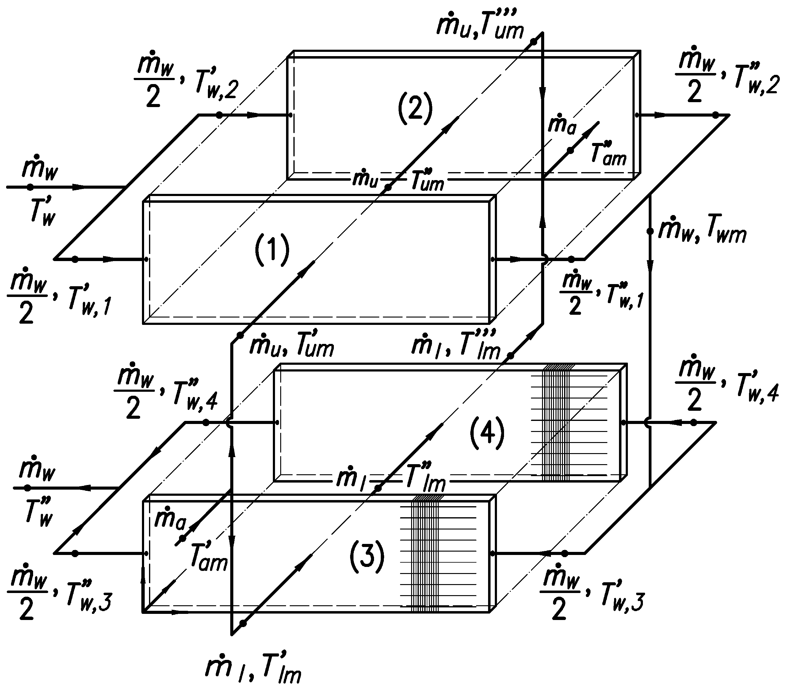
An analytical mathematical model of an automobile radiator with two rows of pipes was developed. The HTCs in the first and second tube row were calculated using heat transfer correlations, which were found based on CFD (computational fluid dynamics) simulations. The flow diagram of the coolers analysed in the study is depicted in Figure 1.
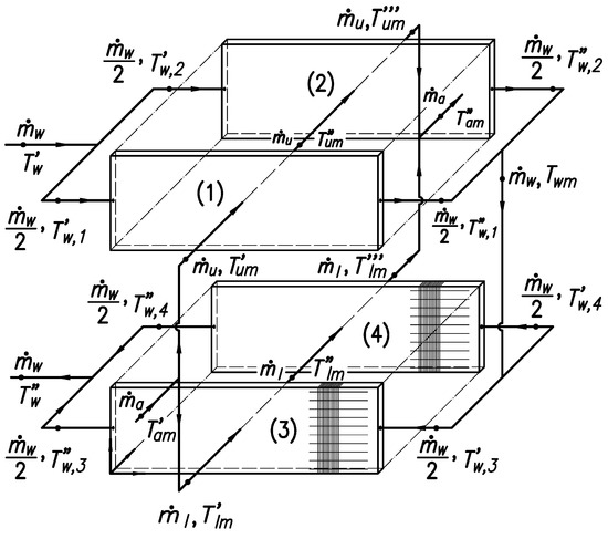
Figure 1.
Flow arrangement of the car radiator analysed in the study: the two-pass car radiator with two rows of tubes consists of the first tube row in the first pass (1), second tube row in the first pass (2), first tube row in the second pass (3), and second tube row in the second pass (4).
The flow rate of the water to the engine cooler is divided into two equal parts flowing through both rows of pipes in the first pass. The starting point for building a mathematical model of an engine cooler is a single-pass of the double-row PFTHE (first pass in the two-pass PFTHE with two tube rows) (Figure 2).
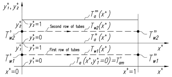
Figure 2.
Two rows of tubes in a single-pass heat exchanger.
2.1. Analytical Model for the First Row of Pipes
The governing energy conservation equations for the water and air for the tube situated in the first row are
where , dimensionless coordinates , Cartesian coordinates (Figure 2) the water temperature in the tube in the first row, the temperature of the air in the first row of pipes.
Two local dimensionless coordinate systems were introduced and (Figure 2). The following expression determines the average air temperature over the first-row width
The number of heat transfer units (NTU) on the water-side and air-side is defined as follows
where , the total number of pipes in the first row of the first pass, outer surface area of the bare pipes in the first row of the first pass, the outer circumference of the plain tube, length of a tube in the PFTHE. The symbol is the average specific heat of the water in the temperature range from to and the average specific heat of the air in the temperature range from to (Figure 2).
The overall HTC is calculated using the expression
where , the inner surface area of the pipes in the first row of the first pass, the inner circumference of the tube, HTC at the inner surface of the pipe, mean surface area of the plain pipe in the first row, the thickness of the tube wall, the thermal conductivity of the tube material.
The equivalent HTC , considering the heat exchange through the fins fixed to the outer surface of a plain tube, is given by
where air-side HTC in the first row of tubes in the first pass, fin surface area, tube surface area between fins, fin efficiency.
The boundary conditions for differential Equations (1) and (2) are
The solution to Equations (1) and (2) with boundary conditions (7) and (8) is
The air temperature after the first row of pipes is obtained from Equation (10) after substitution
The temperature in Equation (11) is defined by Equation (9). The mean air temperature behind the first row of pipes is obtained from its definition
where B is as follows:
The temperature distribution of water and air in the first tube row can be determined using Equations (9)–(13).
2.2. Analytical Model for the Second Row of Pipes
The relevant differential equations for the second row of pipes are
where
The overall HTC can be calculated using Equation (5), in which the HTC is to be substituted by . Expression (6) is used to calculate the effective air-side HTC , but instead of the HTC, , the HTC for the second row of pipes must be substituted.
The average air temperature across the width of the second tube row is determined as follows
The water temperature at the inlet to the second row of pipes is , and the air temperature in front of the second row of tubes is equal to the outlet temperature of the air from the first row of pipes. Thus, the boundary conditions are as follows:
The solution to Equations (14) and (15) under boundary conditions (18) and (19) is
where
The coefficient is given by Equation (13). The expression for air temperature after the second row of pipes (Figure 2) is obtained from Equation (21), taking into account that . After substitution of Equation (20) into Equation (21) and transformations, the following expression for the air temperature behind the second tube row is obtained
The mean air temperature leaving the second tube row is calculated as follows
When the air-side HTC in the first pipe row is equal to the HTC in the second pipe row, then D = B and the denominator (D−B) is zero. When D = B, Equation (20) requires transformation. Writing Equation (20) as
and applying the L’Hôpital rule to an expression where, at D = B, the numerator and the denominator are equal to zero, one obtains
where z = D−B.
Taking into account the relation (26) for D = B (i.e., for ) in Equation (25) gives
where .
If , then the air temperature after the second row of pipes is obtained with Equation (23) after taking into account the relation (26)
where the symbol C is as follows:
3. An Analytical Model of an Internal Combustion Engine Radiator
The equations derived for the single-pass double-row PFTHE, taking into account the different HTCs in individual tube rows, were used to develop an analytical model of the entire radiator depicted in Figure 1. This radiator is used in spark engines with a displacement capacity of 1600 cubic centimeters.
A description of the radiator construction made of round tubes is presented in [10], and the radiator built of oval tubes in [9]. First, the temperatures and of the liquid at the outlet from the first pass of the cooler are calculated. Water from the first and second row of pipes is mixed in the reversing manifold connecting the outlet from the first pass with the inlet to the second pass.
The water mixture with temperature (Figure 1) feeds the second pass of the automobile radiator. The water mass flow rate is the same as in the first pass. The stream of the water is divided into two equal parts flowing through the first and second tube rows. The air flows evenly across the entire radiator cross-section. The rate of the air mass flow across the first (upper) pass is and that of the second (lower) pass is . The symbol is the mass flow rate of air in front of the radiator. The symbols and are the respective numbers of pipes in the first and second passes in the first row of tubes. The numbers and are equal to ten and nine, respectively. Thermal calculations of the second (lower) pass were carried out analogously to those of the first (upper) pass. The comparison of characteristics of oval and round tube are shown in Table 1.

Table 1.
Characteristics of finned tubes in the heat exchanger from oval and round tubes.
The thermal conductivity of aluminium tubes and fins was assumed to be W/(m·K).
4. The Air-Side Heat Transfer Correlations
The air-side HTCs were estimated by CFD simulation using ANSYS CFX. The method of determining the correlations for the average Nusselt number in the individual row of tubes and the whole radiator was presented in [19].
Nusselt number correlations for PFTHE from oval and round pipes are given below:
- oval pipe radiator
The Nusselt number is defined as , where is the thermal conductivity of the air. The Reynolds number on the air side is based on the hydraulic diameter and air velocity at the minimum flow area. The hydraulic diameter for the analysed oval pipe cooler was mm. The exponent of the Reynolds number is very small, which indicates that the average Nusselt number in the first row is almost constant. A constant Nusselt number is a characteristic feature of hydraulically and thermally developed laminar flow. The effect of vortices forming near the forward and backward stagnation point is more pronounced in the second tube row, as the power exponent of the Reynolds number is larger than in the first row. The heat transfer correlation (32) for the average Nusselt number in a two-row bundle is similar to the expression for the average Nusselt number on a flat surface for a thermally and hydraulically developing laminar flow, for which the power exponent of the Reynolds number is 1/3. The following are heat transfer correlations for calculating the Nusselt number on the air side for an engine radiator manufactured from circular tubes.
- round pipe radiator
A comparison of correlations (33) and (34) demonstrates that laminar flow predominates in the first row of round tubes, as the exponent of the Reynolds number is low and equals 0.2414. In the second row of pipes, there are vortexes at the front and back of the pipe, and the exponent of the Reynolds number is higher and amounts to 0.5499. However, the average Nusselt number in the first row is higher than that in the second row, which is mainly due to the inlet section in the gap formed by the two adjacent fins, characterized by very high heat transfer coefficients on the fin surfaces. As a result, the heat flow rate transferred to the air in the first row is higher than that in the second row. The reduction of the heat transfer from the pipe surface and the fins in the second pipe row is strongly influenced by the vortexes forming near the front and backward stagnation point on the pipe surface. The rotating air has a temperature close to that of the fin and pipe surface, and from the point of view of heat exchange, these are dead zones.
The comparison of heat flow rates obtained by the method developed with the experimental results was conducted for two various car radiators. The flow system of both radiators is the same (Figure 1). The first radiator is manufactured from circular pipes and the second one from oval pipes.
5. The Liquid-Side Heat Transfer Correlations
One of the objectives of this study is to illustrate that by the use of theoretical relationships to calculate the HTC on the inner surfaces of the heat exchanger pipes and the use of the liquid-side heat transfer correlations determined by CFD modelling, very similar results can be obtained as with experimental HTCs. By using known and experimentally tested correlations to calculate HCTs, experimental research costs can be significantly reduced or even eliminated entirely. Therefore, Gnielinski’s formulas presented in the VDI (Verein Deutscher Ingenieure) Heat Atlas [20] were applied to determine the HTC in the laminar flow and relationships proposed by Taler [21] for transition and turbulent flow in tubes. In the range of the laminar flow regime, the average HTC along the entire length of pipe , assuming that the velocity distribution at the cross-section of the pipe inlet is flat and the liquid flow is hydraulically and thermally developing, is determined by the following formula [20]
The symbol designates the average Nusselt number in the developed laminar flow
The second Nusselt number represents the Lévêque solution [4] for developing flow over the planar surface, and was derived numerically for the constant liquid velocity at the tube inlet
The Nusselt number in the transition and turbulent flow range was evaluated by the Taler correlation [21]:
The Darcy–Weisbach friction factor for turbulent flow, when was calculated by the Taler equation [22]:
The relationship for the coefficient of friction for the transition region was obtained by the linear interpolation [22] between the value for and
The Reynolds number on the water side was determined using hydraulic diameter . The hydraulic diameter was mm for oval tubes and mm for circular tubes. The water’s physical properties were evaluated at the average temperature .
6. Experimental Results
Using the results of experimental research on two car radiators, one of which is made of oval tubes and the other of round tubes, heat transfer correlations on the air side were found. The HTCs on the inner surface of pipes were calculated using Equations (36)–(42), depending on the laminar, transition, or turbulent flow mode.
6.1. Engine Cooler Made of Oval Tubes
Experimental research was conducted at a test facility presented in [10]. The unknown parameters, the coefficient, and power exponent of the Reynolds number were determined based on 48 measurement series. The velocity of the air before the radiator varied between 0.98 and 2.01 m/s, and the water volume flow rate at the radiator inlet was between 627 and 2421 litres/h. The air temperature in front of the PFTHE ranged from 11.0 to 15.0 °C, and the temperature of the water at the car radiator inlet was between 59.6 and 72.2 °C. The air side Reynolds number ranged from 150 to 330, and the water-side Reynolds number in the first (upper) pass varied from 2500 to 11,850. When determining the correlations on the air-side, the water-side HTC was calculated using Equations (36)–(42). The following Equation for the Nusselt number on the air side was found using the experimental data
where the parameters and are
Numbers with a sign in Equation (44) represent half of the 95% confidence interval.
6.2. Engine Cooler Made of Round Tubes
Flow and heat measurements of a car radiator made of round pipes were carried out on the stand presented in paper [10]. The air-side heat transfer correlation was determined using 70 measurement sets. In the measurement tests, the air velocity, flow rate, and temperature of the water at the car radiator inlet were changed.
The velocity of the air changed between 0.74 and 2.27 m/s, and the water flow rate at the radiator inlet was between 300 and 2410 litres/h. The air temperature before the car radiator ranged from 3.6 to 15.5 °C, and the temperature of the water at the inlet to the radiator was between 50 and 72 °C. The water flow regime changed from laminar to transitional and then to turbulent during testing. The air-side Reynolds number ranged from 150 to 560. The Reynolds number on the water side in the first pass of the heat exchanger varied from 1450 to 16,100 during the test. The water-side HTC in round tubes was evaluated using relationships (36)–(42). The following Equation for the Nusselt number on the air side was obtained by the least-squares method
Based on the 70 data series, the following values of parameters and were found
Numbers with a sign in Equation (46) represent half of the 95% confidence interval.
7. Analysis and Discussion of Heat Flow Rates from Water to Air Transferred in the Entire Heat Exchanger and Individual Rows of Pipes
For a radiator constructed from oval pipes, the results of mathematical modelling and measurements are presented versus the Reynolds number on the air side for two selected volume flow rates of water litres/h and litres/h. For a car radiator built of round tubes, the results of tests and calculations are presented versus the water Reynolds number for the first pass of the heat exchanger for the preset velocity of the air before the radiator equal to 2.27 m/s.
7.1. Engine Cooler Made of Oval Tubes
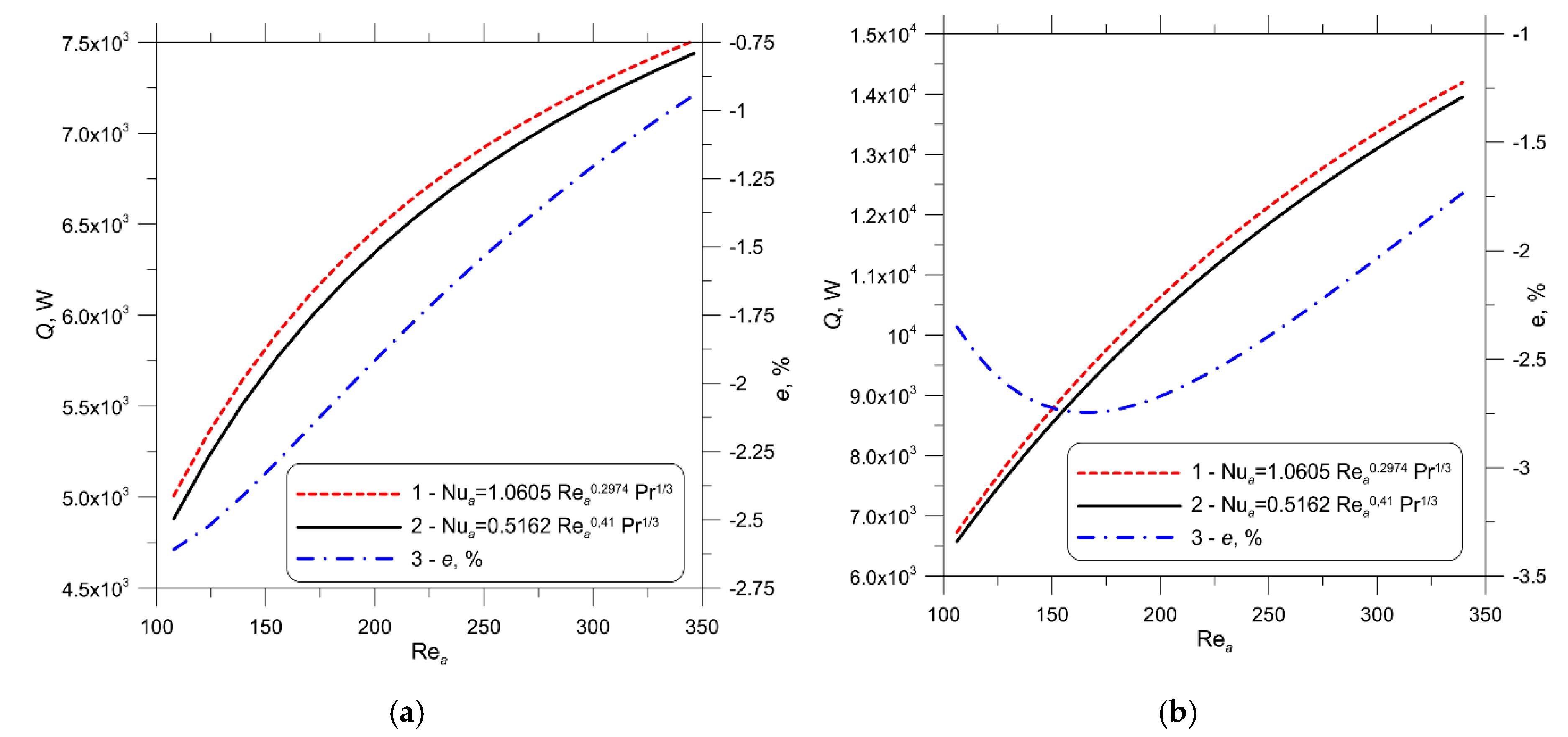
The thermal capacity of the radiator was calculated by using the radiator analytical model developed in this study, assuming the uniform air-side HTC on both rows of pipes. Figure 3a shows heat flow rates estimated using the analytical model of the PFTHE for mean volume flow rate liters/h, average air temperature at the inlet , and average water inlet temperature . The mean values , , and were calculated for seven measured data series. The water flow in the tubes was laminar. The water side Reynolds number in the first (upper) pass ranged from 1,222 to 1287, and in the second pass from 1358 to 1430. The air velocity w0 varied between 0.71 m/s and 2.2 m/s. Figure 3b presents heat flow rates obtained for the following data: liters/h, , and . The water flow in the pipes was turbulent as the Reynolds number in the first pass of the cooler varied from 5238 to 5440, and in the second pass ranged from 5820 to 5883. The air velocity in front of the heat exchanger changed from 0.71 m/s to 2.2 m/s.
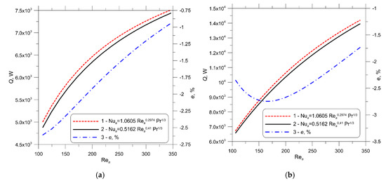
Figure 3.
The heat transfer rate from water to air in an engine radiator made of oval tubes with an equal HTC on the air side of the entire radiator; (a) litres/h, and ; (b) litres/h, and ; 1—air side equation for obtained from the CFD modelling, 2—empirical air side equation for , 3–relative difference e.
The HTC on the water side was calculated with a mathematical model of a radiator using Equations (36)–(42). The air-side HTC was calculated using Equation (32) based on CFD simulation (Equation (1) in Figure 3) or empirical Equation (43) (Equation (2) in Figure 3).
The inspection of the results depicted in Figure 3a,b illustrates that the absolute value of the difference e does not exceed 2.75%. The heat flow rates based on the measurement data and CFD simulations were calculated as follows
where -the average specific heat of the water in the interval between the outlet (Equation (47)) or (Equation (48)) and inlet water temperature , -volumetric water flow rate measured at the car radiator inlet.
The relative difference e was obtained from the following Equation
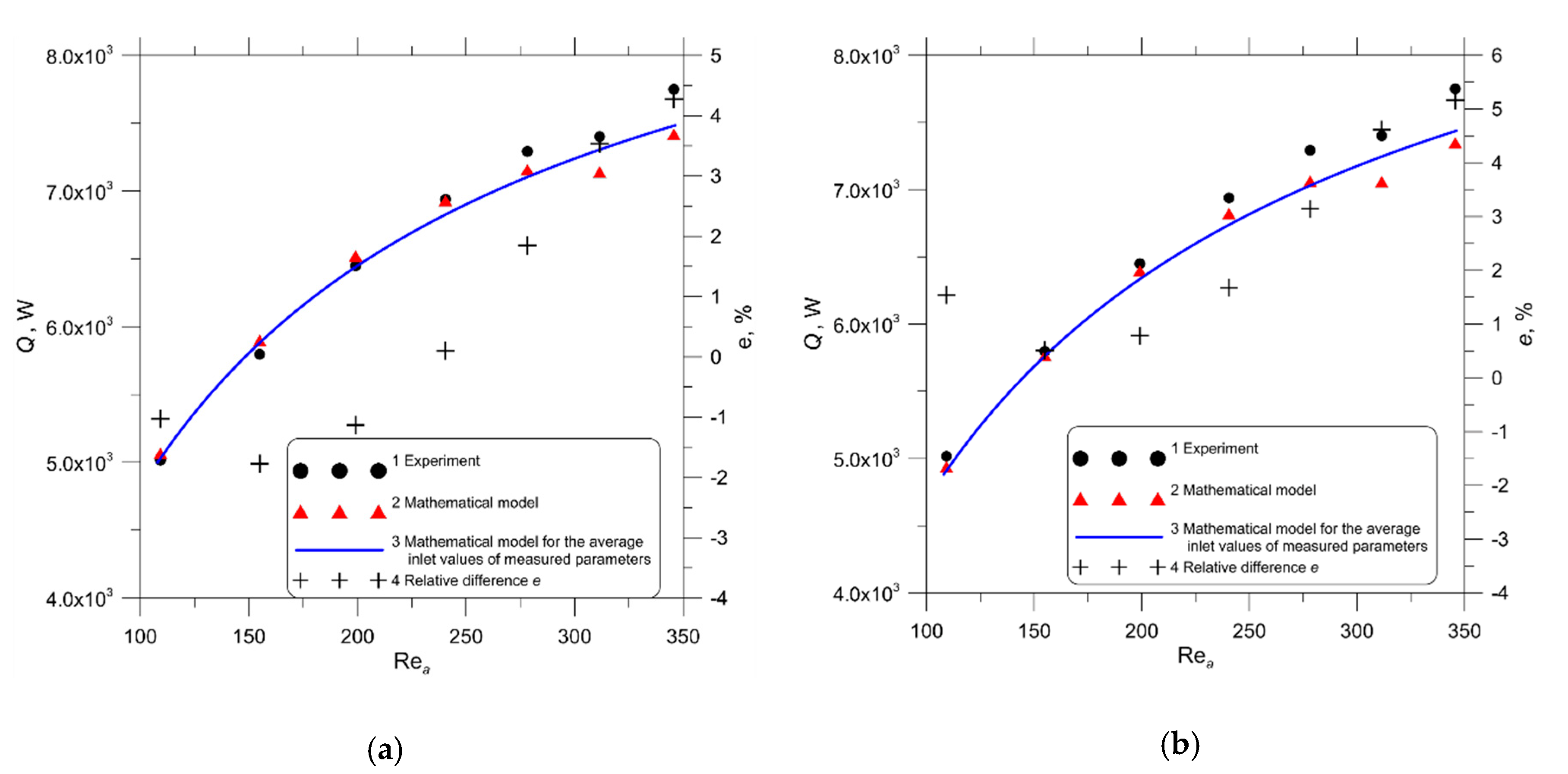
Figure 4 shows the measurement and calculation results for the heat transfer rate for the seven measurement series and the calculation results for the averaged measurement data: litres/h, , and . The heat flow rate values (Entries 2 and 3) were determined using an analytical model of the engine cooler, in which the water-side HTC was calculated using Equations (36)–(42). Because of the small water flow rate, the flow regime of water in the heat exchanger pipes was laminar. The HTC on the air side was determined either by Equation (32) obtained from CFD simulation (Figure 4a) or by empirical correlation (43) (Figure 4b). The values of the relative difference , calculated using Equation (49), are also shown in Figure 4. The analysis of the results shown in Figure 4a,b indicates that the use of correlation (32) based on CFD modelling for the calculation of the air-side HTC gives an excellent agreement between the calculated and measured heat flow rates. When using both CFD-based Equation (32) or empirical Equation (43), the relative differences range from about (−1.5%) to about 5.2%.
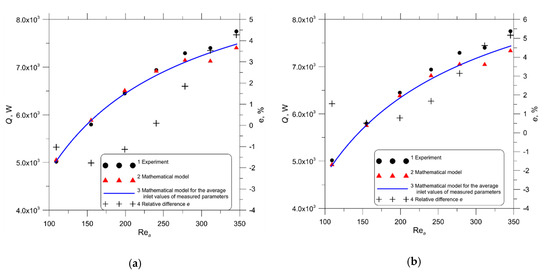
Figure 4.
Heat flow rate transferred from hot water to cool air in the car radiator; 1: values determined using the measurement results, 2: heat flow rate obtained for the air-side Nusselt number estimated by CFD simulation (a) or empirical correlation (b), 3: heat flow rate calculated using the CFD-based Equation (a) or empirical Equation (b) and the average input data from seven measurement series: liters/h, and , 4: the relative difference between and (between 1 and 2).
Figure 5 shows a similar comparison as in Figure 4, but for other averaged measurement data: litres/h, and . Due to the higher flow rate of water flow through a car radiator equal to liters/h, the flow regime of water in pipes was turbulent. The water-side Reynolds number in the first pass pipes was between 5238 and 5440. In the lower pass, the Reynolds number was higher due to the smaller number of pipes and varied between 5820 and 5883.
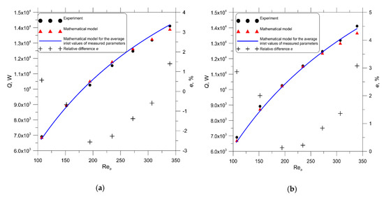
Figure 5.
The thermal output of the car radiator; 1: values determined using the measurement results, 2: thermal output calculated with the air-side Nusselt number obtained by CFD simulation (a) or empirical Equation (b), 3: thermal output obtained using the CFD-based correlation (a) or empirical correlation (b) and the average input data from seven measurement series: litres/h, and , 4: the relative difference between and .
The analysis of the results presented in Figure 5a,b shows that the thermal output of the car radiator calculated using a mathematical model is very close to the output determined experimentally, both for the relationship for the air-side HTC determined by computer simulation (Figure 5a) and for the empirical correlation for HTC determined by experimental tests (Figure 5b). The relative differences between the measured and calculated capacities are in the range of about (−2.5%) to 4.5% (Figure 5).
It was found that the correlation for the air-side Nusselt number determined for the entire double-row radiator based on CFD modelling provides a perfect match between the calculated and measured thermal output (Figure 4 and Figure 5). Then, the heat flow transferred in the first and second rows of pipes in both radiator passes was calculated, taking into account different first and second-row HTCs. The following equations were applied to calculate the capacity in each row of pipes in both passes in the car radiators:
The total capacity of the car radiator was evaluated as follows:
The designations mean the thermal capacity of the specific pipe row (Figure 1) with a uniform HTC throughout the car radiator given by Equation (32). The symbol stands for the thermal capacity in a particular row, with different HTCs in the first and second pipe rows. The first-row HTC was evaluated, applying Equation (30) and in the second row by using Equation (31). When the HTC on the air-side is constant across the entire radiator, then in Equations (50)–(54), is assumed, and if the HTCs in the first and second tube rows are different, then should be used. The relative differences between the thermal capacity with different HTCs and the capacity with constant HTC across the entire car radiator were also determined:
The relative difference for the entire PFTHE was determined by a similar formula
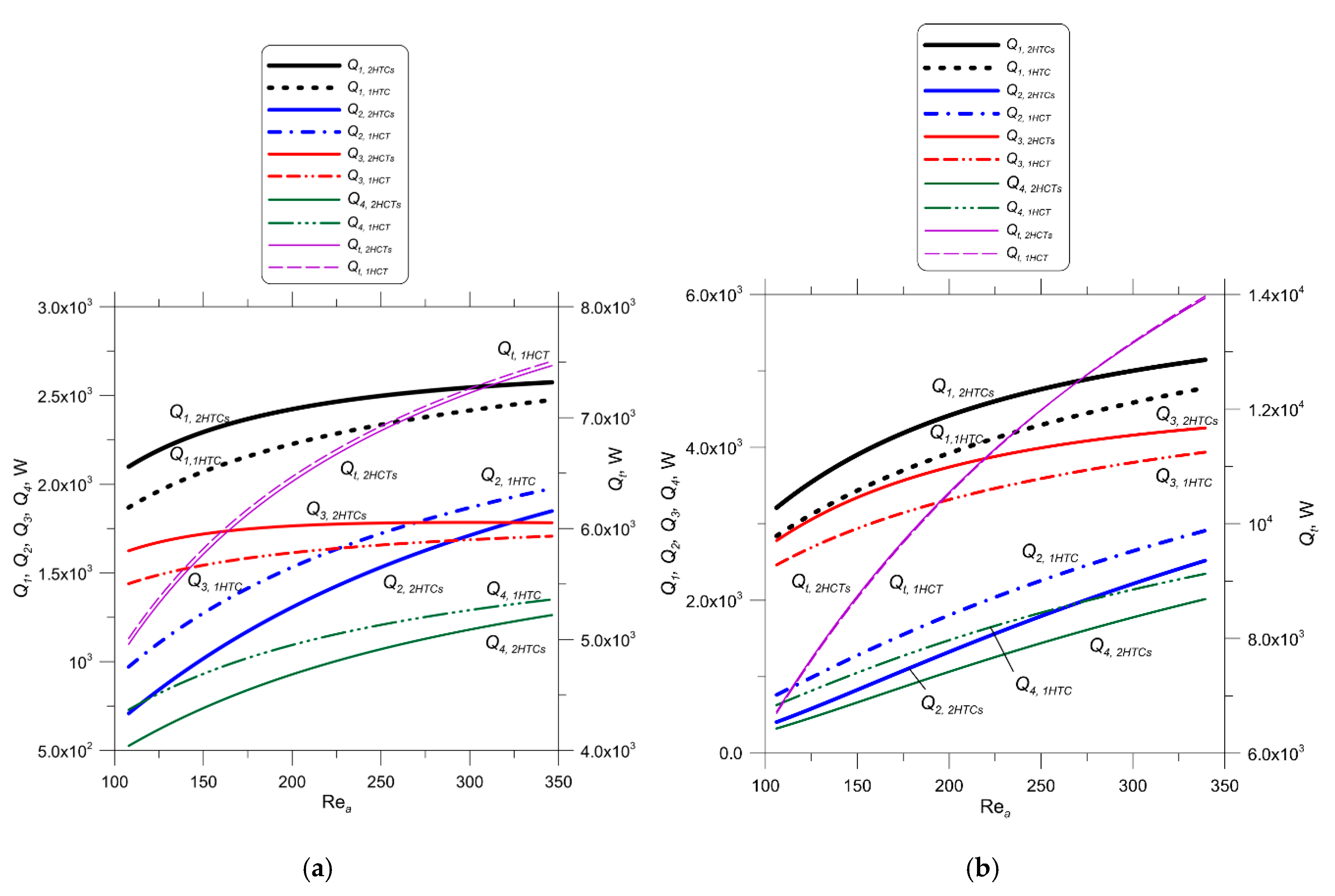
A comparison of the thermal output of the specific tube rows and the radiator heat output for the uniform HTC throughout the radiator and different HTCs in individual tube rows are depicted in Figure 6a for liters/h and in Figure 6b for litres/h.
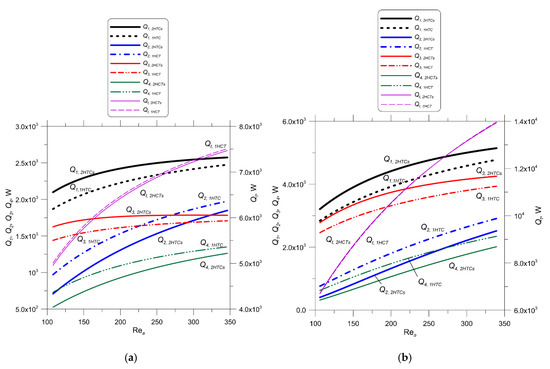
Figure 6.
Comparison of thermal outputs of the specific pipe rows and whole-car radiator considering that the air-side HTC is constant in both pipe rows with the corresponding thermal outputs for different HTCs in the first and second pipe rows; (a) litres/h, and , (b) litres/h, and ; , : thermal output of the specific pipe row (Figure 1) adopting the same correlation (32) for the Nusselt number on the air side, , : thermal outputof a specific pipe row for different correlations for the air side Nusselt number (Figure 1); Equation (30) was used for the first row and Equation (31) for the second row of tubes, : car radiator output for constant HTC calculated from Equation (32) for all rows of pipes, : car radiator output for different HTCs; Equation (30) was used for the first tube row and Equation (31) for the second tube row.
The inspection of the results presented in Figure 6a,b shows that the thermal output of the radiator is almost identical for a uniform HTC throughout the radiator and different HTCs in both rows of pipes. As shown in Figure 5 and Figure 6, the radiator capacity determined by applying an analytical model of the engine cooler using the CFD-based air-side equation for the Nusselt number is in line with the measurements. It can also be seen that the thermal output of the first and second tube rows in both passes of the radiator is significantly higher for different correlations for the air-side Nusselt compared to the heat flow rates obtained assuming the same HTC in both pipe rows.
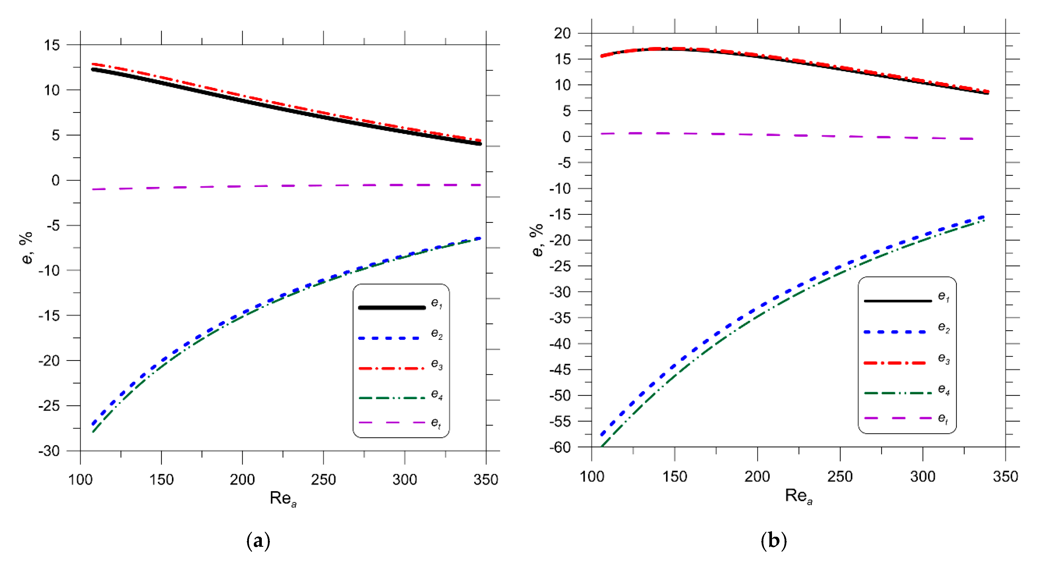
The heat capacity of the heat exchanger is almost identical to the same and different HTCs for both rows of pipes (Figure 5 and Figure 6). Uniform HTC for two rows of pipes was found from the condition of equal air temperature rise in the whole exchanger determined from CFD modelling and analytical formula [19]. Considering that the air temperature gain in both pipe rows is equal to the sum of the temperature rise in the first and second pipe rows, it can be expected that the heat output of the entire heat exchanger will be almost identical to the uniform and different HTCs. Figure 7a,b illustrate the higher heat absorption by the air in the first pipe row and the considered reduction of the heat flow rate in the second pipe row if different correlations for the Nusselt numbers are adopted compared to the respective outputs of the individual rows with uniform HTC.

Figure 7.
The relative differences between thermal outputs of specific tube rows for different and constant HTCs; (a) litres/h, and , (b) litres/h, and .
Figure 7a,b show that considerable discrepancies in the exchanged heat flow through the first and second rows of pipes for uniform and different HTCs are higher for a larger volume flow rate passing through the cooler. The differences in the thermal capacities of individual pipe rows with equal and different HTCs for both pipe rows become smaller as the Reynolds number on the air side increases.
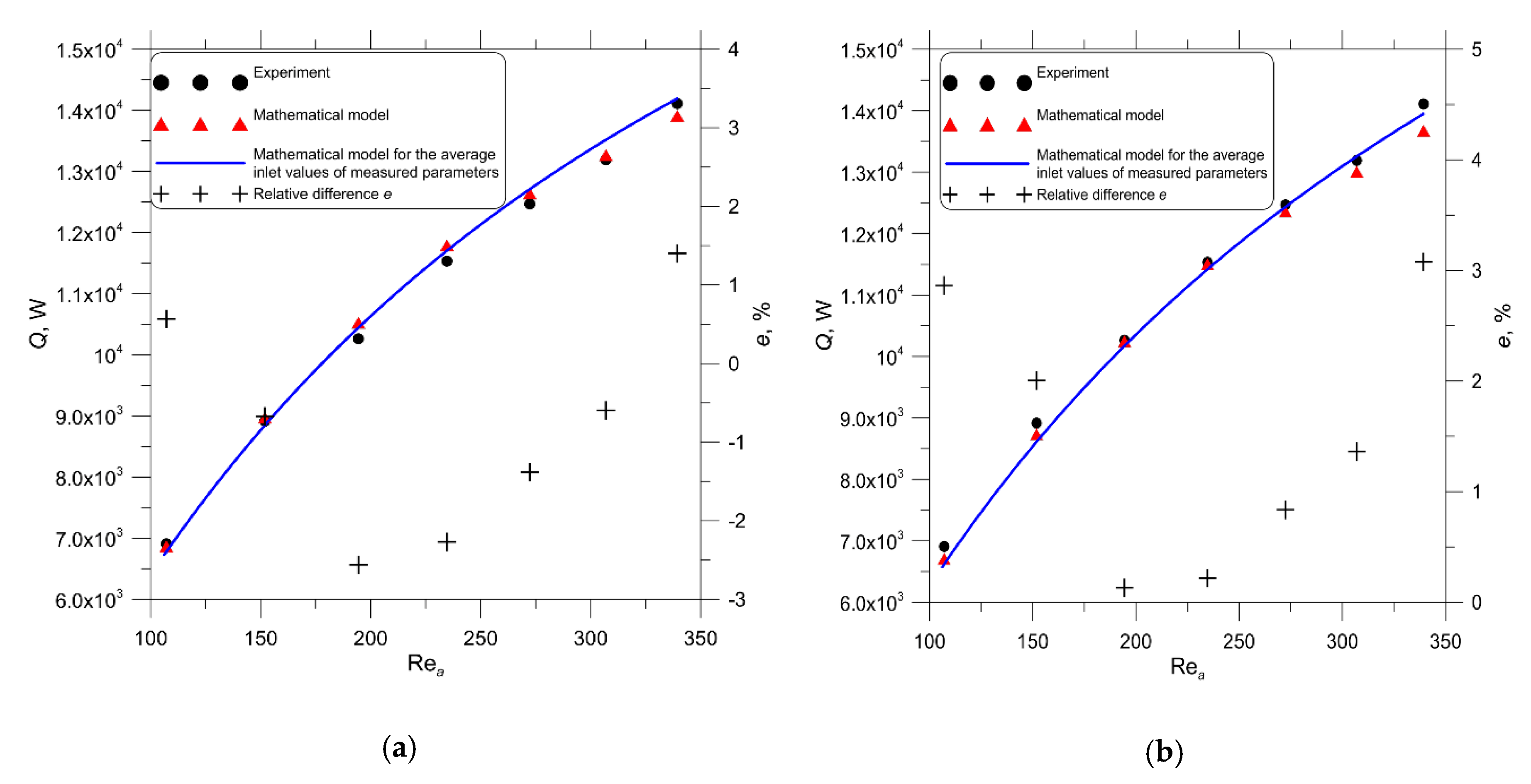
7.2. Engine Cooler Made of Circular Tubes
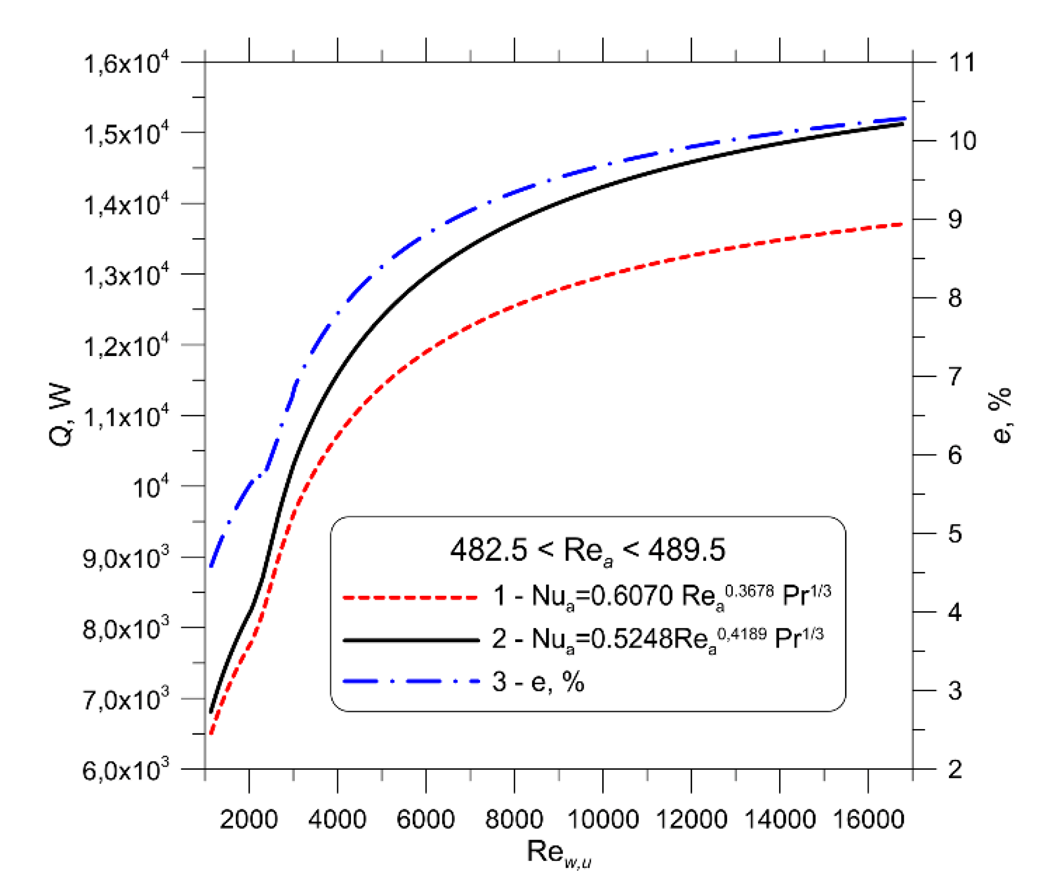
Figure 8 depicts a comparison of the thermal output of the car radiator for the CFD-based air-side correlation (35) and empirical correlation (45) for averaged measurement data: m/s, , and . The volume flow rate of water at the radiator inlet varied from 309 to 2,406 litres/h. The Reynolds number on the air side changed from 482.5 to 489.5, and the water-side Reynolds number in the first (upper) pass of the cooler varied from 1,834 to 16,084. Examination of the results reported in Figure 8 reveals that the capacity of a round-tube radiator calculated for the empirical correlation with the air-side Nusselt number exceeds the capacity of the radiator calculated using the correlation with the Nusselt number on the air side obtained by CFD modelling. The relative difference calculated using Equation (49) is about 5% for a Reynolds number on the water side of 1800 and about 10% for a Reynolds number of 16,000 (Figure 8).
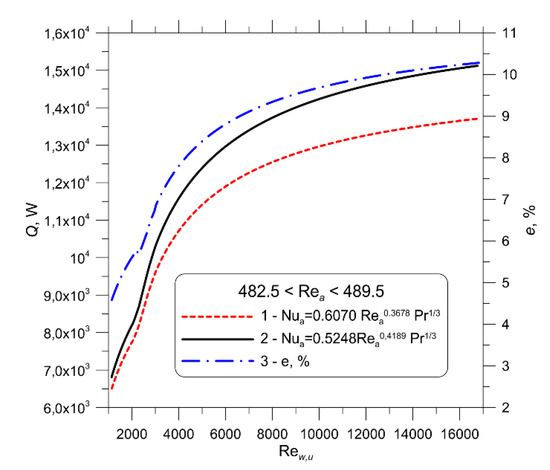
Figure 8.
The heat flow rate from water to air in an engine cooler constructed from round tubes with an equal HTC on the air side of the entire radiator versus the first-pass Reynolds number on the water side; 1: air-side correlation for based on CFD modelling, 2: air-side relationship for based on experimental data, 3: relative difference e.
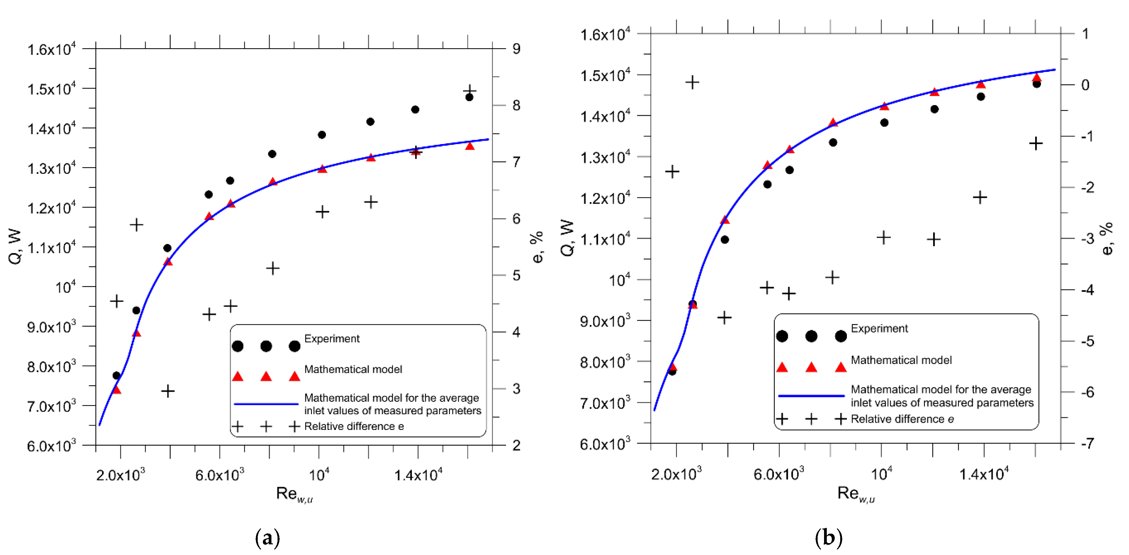
The analysis of the results shown in Figure 9a indicates that the relative difference between the radiator output determined experimentally and that calculated using a mathematical model of the radiator with a correlation to the air-side Nusselt number obtained by CFD modelling is between 3% and about 8.3%. In the case when the air-side relationship is determined experimentally, the relative difference is smaller and is in the range from −4% to 0% (Figure 9b). Figure 10 presents a comparison of the thermal outputs of the individual pipe rows assuming the same air-side HTC in the analytical model of the radiator and different HTCs in the first and second pipe rows.
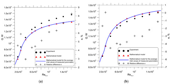
Figure 9.
The comparison of radiator output versus the water-side Reynolds number obtained experimentally and using the mathematical model of the engine cooler with the uniform air-side Nusselt number determined by (a) CFD modelling and (b) empirical correlation; : relative difference.
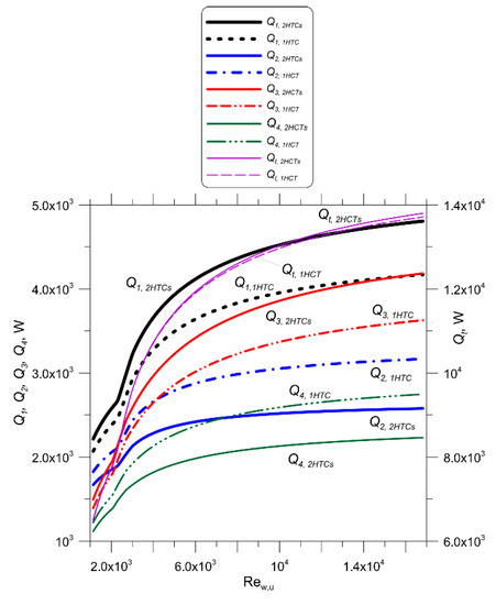
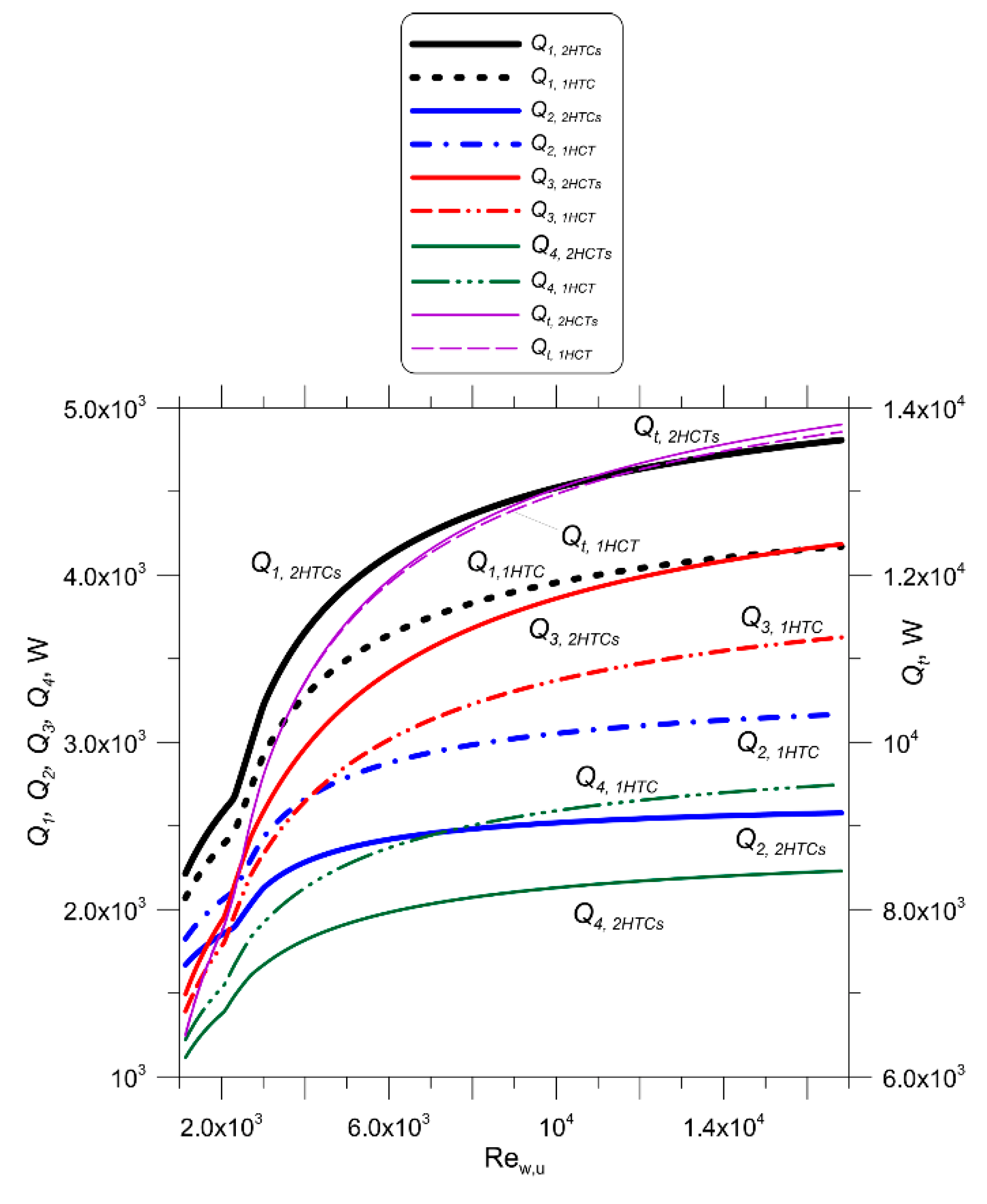
Figure 10.
Comparison of thermal capacities of specific pipe rows and the whole-car radiator supposing that HTC on the air-side is uniform in both pipe rows with the corresponding thermal capacities obtained for different HTCs in the first and second pipe rows; m/s, , and ; , : thermal output of the specific pipe rows (Figure 1) supposing the same Equation (32) for the Nusselt number on the air-side throughout the radiator, , : thermal outputs of individual pipe rows (Figure 1) for different equations for the air-side Nusselt in both pipe rows; Equation (30) was used for the first row of tubes and Equation (31) for the second row, : car radiator output calculated using Equation (32) for all rows of pipes, : car radiator output calculated using different heat transfer correlations for the first and second tube rows.
The air in the first pipe row has a much larger heat flow rate assuming different HTCs in the first and second pipe rows compared to the heat flow rate determined considering an even HTC throughout the heat exchanger (Figure 10 and Figure 11).
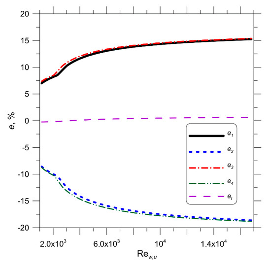
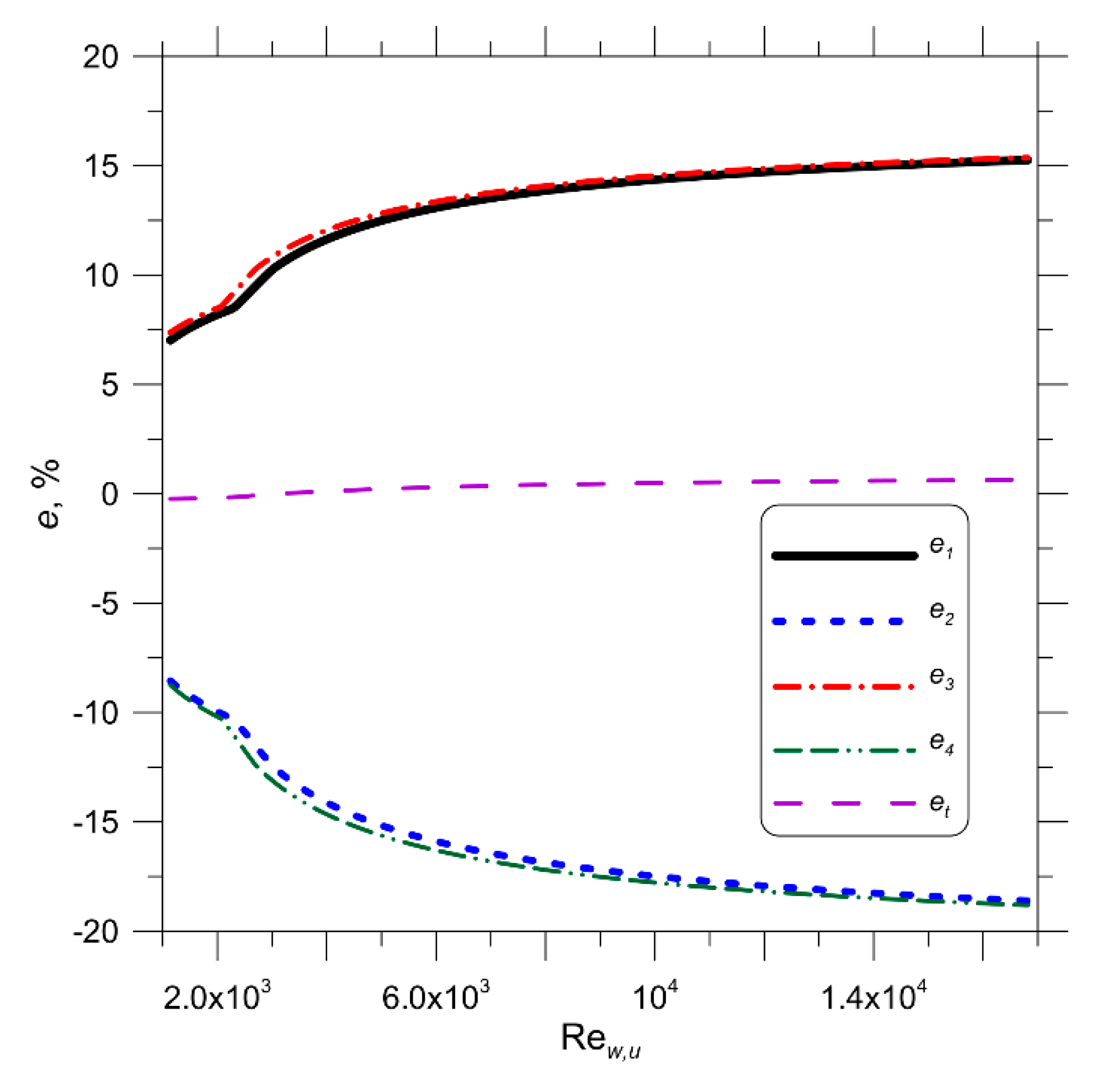
Figure 11.
The relative differences and between thermal outputs of individual tube rows and the entire car radiator for different and uniform HTCs calculated using Equations (55) and (56); m/s, , and .
The relative differences and are approximately 7.5% for equal to 1000 and increase with to about 15% for the Reynolds number equal to 18,000. The relative differences of and are approximately −8% for equal to 1000 and decrease with to approximately −18% for the Reynolds number equal to 18,000. The results depicted in Figure 10 and Figure 11 show that the radiator thermal output is almost identical for the same and different HTCs on both rows of pipes, despite the various capacities of the first and second rows of tubes.
8. Conclusions
An analytical model of a two-pass automobile radiator with two rows of pipes has been developed. Correlations determined by CFD modelling should be used to determine the air-side HTC. Radiators made of round and oval pipes were analysed. Mathematical models of car radiators were proposed, in which only one average HTC for the entire heat exchanger was used, as well as various correlations for calculating the air-side HTCs for the specific of rows of pipes. Calculation of the PFTHE with various HTCs for each row of tubes makes it possible to calculate more accurately the thermal output of individual rows of pipes, which, for example, allows designing a PFTHE with an optimum tube row number. The relationships based on the numerical solution of the equations of momentum and energy conservation for the fluid were used to calculate the HTC on the inner surface of the pipes. The water flow in the tubes may be laminar, transitional, or turbulent. The results of the calculations of both tested car radiators were compared with experimental data. The agreement between calculation and measurement results is excellent. The proposed method of calculating PFTHEs is attractive because of the elimination of costly experimental research necessary for the experimental determining of the heat transfer correlations on the air and water side.
The main achievements presented in the article are as follows:
- An exact analytical model of a single-pass double-row heat exchanger with different heat transfer coefficients on the first and second rows of pipes.
- Exact analytical model of a two-row, two-pass car radiator (plate-fin and tube heat exchanger (PFTHE)) with different heat transfer coefficients for the first and second tube rows.
- Calculation method of PFTHE without using empirical heat transfer correlations on the water and air sides.
- The results of extensive experimental research on two car radiators, one of which is made of oval tubes and the other of round tubes.
- The water flow in the pipes can be laminar, transient or turbulent while maintaining the continuity of the heat transfer coefficient when changing the flow regime. CFD modeling of all three flow ranges would be difficult.
Author Contributions
Conceptualization, J.T. and D.T.; methodology, D.T.; software, M.T. and D.T.; validation, J.T., D.T. and M.T.; formal analysis, J.T.; investigation, M.T. and D.T.; resources, M.T.; data curation, M.T.; writing—original draft preparation, D.T. and J.T.; writing—review and editing, J.T., D.T. and M.T.; visualization, D.T. and M.T.; supervision, J.T.; project administration, D.T.; All authors have read and agreed to the published version of the manuscript.
Funding
This research received no external funding.
Conflicts of Interest
The authors declare no conflict of interest.
References
- Shah, R.K.; Sekuli, D.P. Fundamentals of Heat Exchanger Design; John Wiley & Sons: Hoboken, NJ, USA, 2003. [Google Scholar]
- Kakaç, S.; Liu, H.; Pramuanjaroenkij, A. Heat Exchangers. Selection, Rating, and Thermal Design, 3rd ed.; CRC Press-Taylor and Francis Group: Boca Raton, FL, USA, 2012. [Google Scholar]
- Kuppan, T. Heat Exchanger Design Handbook, 2nd ed.; CRC Press Taylor and Francis Group: Boca Raton, FL, USA, 2013. [Google Scholar]
- Taler, D. Numerical Modelling and Experimental Testing of Heat Exchangers; Springer: Berlin/Heidelberg, Germany, 2019. [Google Scholar]
- Kim, N.-H.; Yun, J.-H.; Webb, R.L. Heat Transfer and Friction Correlations for Wavy Plate Fin-and-Tube Heat Exchangers. J. Heat Transf. 1997, 119, 560–567. [Google Scholar] [CrossRef]
- Kim, N.H.; Youn, B.; Webb, R.L. Air-Side Heat Transfer and Friction Correlations for Plain Fin-and-Tube Heat Exchangers With Staggered Tube Arrangements. J. Heat Transf. 1999, 121, 662–667. [Google Scholar] [CrossRef]
- Wang, C.-C.; Hsieh, Y.-C.; Lin, Y.-T. Performance of Plate Finned Tube Heat Exchangers Under Dehumidifying Conditions. J. Heat Transf. 1997, 119, 109–117. [Google Scholar] [CrossRef]
- Halıcı, F.; Taymaz, I.; Gunduz, M.; Halici, F. The effect of the number of tube rows on heat, mass and momentum transfer in flat-plate finned tube heat exchangers. Energy 2001, 26, 963–972. [Google Scholar] [CrossRef]
- Taler, D. Mathematical modeling and experimental study of heat transfer in a low-duty air-cooled heat exchanger. Energy Convers. Manag. 2018, 159, 232–243. [Google Scholar] [CrossRef]
- Taler, D.; Taler, J. Prediction of heat transfer correlations in a low-loaded plate- fin-and-tube heat exchanger based on flow-thermal tests. Appl. Therm. Eng. 2019, 148, 641–649. [Google Scholar] [CrossRef]
- Rich, D.G. The effect of the number of tube rows on heat transfer performance of smooth plate fin-and-tube heat exchangers. ASHRAE Trans. 1975, 81 Pt 1, 307–317. [Google Scholar] [CrossRef]
- Marković, S.; Jaćimović, B.; Genić, S.; Mihailović, M.; Milovancevic, U.; Otović, M. Air side pressure drop in plate finned tube heat exchangers. Int. J. Refrig. 2019, 99, 24–29. [Google Scholar] [CrossRef]
- McQuiston, F.C.; Parker, J.D.; Spitler, J.D. Heating, Ventilating, and Air Conditioning Analysis and Design, 6th ed.; Wiley: Hoboken, NJ, USA, 2005. [Google Scholar]
- Webb, R.L.; Kim, N.H. Principles of Enhanced Heat Transfer, 2nd ed.; CRC Press: Boca Raton, FL, USA, 2005. [Google Scholar]
- Sun, C.; Lewpiriyawong, N.; Khoo, K.L.; Zeng, S.; Lee, P.-S. Thermal enhancement of fin and tube heat exchanger with guiding channels and topology optimisation. Int. J. Heat Mass Transf. 2018, 127, 1001–1013. [Google Scholar] [CrossRef]
- Li, M.; Zhang, H.; Zhang, J.; Mu, Y.; Tian, E.; Dan, D.; Zhang, X.; Tao, W. Experimental and numerical study and comparison of performance for wavy fin and a plain fin with radiantly arranged winglets around each tube in fin-and-tube heat exchangers. Appl. Therm. Eng. 2018, 133, 298–307. [Google Scholar] [CrossRef]
- Nagaosa, R. Turbulence model-free approach for predictions of air flow dynamics and heat transfer in a fin-and-tube exchanger. Energy Convers. Manag. 2017, 142, 414–425. [Google Scholar] [CrossRef]
- Kearney, S.P.; Jacobi, A. Local Convective Behavior and Fin Efficiency in Shallow Banks of In-Line and Staggered, Annularly Finned Tubes. J. Heat Transf. 1996, 118, 317–326. [Google Scholar] [CrossRef]
- Taler, D.; Taler, J.; Trojan, M. Thermal calculations of plate-fin-and-tube heat exchangers with different heat transfer coefficients on each tube row. Energy 2020, 203, 117806. [Google Scholar] [CrossRef]
- Gnielinski, V. Heat transfer in pipe flow, chapter G1. In VDI Heat Atlas, 2nd ed.; Springer: Berlin/Heidelberg, Germany, 2010; pp. 691–700. [Google Scholar]
- Taler, D. A new heat transfer correlation for transition and turbulent fluid flow in tubes. Int. J. Therm. Sci. 2016, 108, 108–122. [Google Scholar] [CrossRef]
- Taler, D. Determining velocity and friction factor for turbulent flow in smooth tubes. Int. J. Therm. Sci. 2016, 105, 109–122. [Google Scholar] [CrossRef]

© 2020 by the authors. Licensee MDPI, Basel, Switzerland. This article is an open access article distributed under the terms and conditions of the Creative Commons Attribution (CC BY) license (http://creativecommons.org/licenses/by/4.0/).