Abstract
Overall heat transfer coefficient, also known as the intrinsic performance measurement of the building, determines the amount of heat lost by a building due to temperature difference between indoor and outdoor. QUB (Quick U-value of Buildings) is a short-term method for measuring the overall heat transfer coefficient of buildings. The test involves heating and cooling the house with a power step and measuring the indoor temperature response in a single night. Ideally, the outdoor temperature during QUB experiment should remain constant. To compare the influence of variable outdoor temperature, the QUB experiments are simulated on a well-calibrated model with real weather conditions. The experiments at varying outdoor temperature and constant outdoor temperature during the night show that the results in both conditions are nearly similar. A ±2 °C increase or decrease in the outdoor temperature during the QUB experiment can change the results in the measured overall heat transfer coefficient by ±5%. QUB experiments simulated during the months of winter show that the majority of results are ±15% of the steady-state overall heat transfer coefficient. The QUB results during the months of summer show relatively large variation. The large errors coincide with the small temperature difference between indoor and outdoor temperatures before the start of QUB experiment. The median error of multiple QUB experiments during summer can be reduced by increasing the setpoint temperature before the start of QUB experiment.
1. Introduction
Significant savings can be achieved in both new and existing buildings. Depending on the level and type of retrofit (deep or shallow) and the type of building, the potential savings can range from 25% to 90% [1]. Due to this potential, building energy efficiency sector received highest percentage (58%) of investments in energy efficiency sector in International Energy Agency (IEA) member countries (including six major emerging economies Brazil, China, India, Indonesia, Russian Federation, and Mexico) in 2017 [2].
Energy efficiency improvements require investments that are justified against the predicted savings. The saving predictions are based on simulation of baseline annual energy consumption and are hardly realized in field over the course of time due to several factors. This difference between estimated energy consumption and the measured energy consumption is usually referred to as ‘Performance Gap’ [3]. Some of the reasons of performance gap are deterioration of building thermal properties, reduction in efficiency of equipment, operation off the designed values, changing weather pattern, changes in operation schedule, occupancy, and inability of simulation tools to cover complete dynamics of building [4]. A study of domestic buildings in the UK shows that savings from building envelope retrofits can be overestimated by 30% when based on calculations only [4]. In case of old buildings, it was shown that the savings from retrofits were overestimated in 77% of cases [4].
A better indicator of building performance is to measure the building parameters, such as overall heat transfer coefficient, solar aperture, building time constants, etc., also known as the intrinsic performance measures [5,6]. The intrinsic performance measures give the performance of building envelope, i.e., heating and cooling losses, free gains, etc., and remain stable with changing weather conditions, operation schedule, occupancy, etc.
The overall heat transfer coefficient , the most popular parameter for building performance measurement [6,7], gives a measure of building heat loss due to temperature difference between the building and its environment [8]:
This includes losses via building surfaces and infiltration. A simple equation presenting the calculation of overall heat loss coefficient from the stated building properties is [6,7]:
where:
| product of heat transfer coefficient of building elements (Ui) and its area (Ai), W/K; | |
| HTB | thermal bridge heat loss coefficient, W/K; |
| infiltration losses, W/K. |
Equation (1) is based on the thermal properties of the building that are used in design phase but that may change due to wear and tear, transfer of moisture through building envelope, and missing insulation layers. The overall heat transfer coefficient is, therefore, determined using onsite test methods. The common onsite test methods discussed in the literature are classified as [8,9]:
- -
- long-term or short-term;
- -
- intrusive or non-intrusive;
- -
- controlled or non-controlled;
- -
- measurement of individual building components such as walls, roofs, etc. or of entire building.
Based on the available data and purpose of the identification, the methods can be either steady-state or dynamic.
Co-heating, calorific test method, and flow meter test are long-term, steady-state test methods. Co-heating test method is the most common long-term method; it is considered as a reference method used as a benchmark for the other methods. The co-heating test method involves heating the building at a constant temperature and measuring the required power input, the solar radiation, and outdoor temperature during the test [9]. The overall heat loss coefficient is estimated using [3]:
where
| heating power supplied to keep the temperature constant, W; | |
| solar power received by the building, W; | |
| overall heat transfer coefficient, W/K; | |
| indoor temperature of the building, K or °C; | |
| ambient temperature of the external environment, K or °C. |
The required time duration for co-heating is at least two weeks but can increase up to a month. Since the method is performed in empty buildings and the duration is long, it is difficult to employ it as part of regular energy audits. Short-term test methods can be used to circumvent the problem of long duration. ISABELE (In-situ Assessment of the Building Envelope Performances), PSTAR (Primary and Secondary Terms Analysis and Renormalization), and QUB (Quick U-value of Buildings) are some of the short-term, dynamic test methods [10,11,12].
PSTAR (Primary and Secondary Terms Analysis and Renormalization) is one of the earliest short-term test methods, with pioneering work by K. Subbarao [11]. The test duration for PSTAR is three nights and four days. It involves the first step to attain steady-state conditions, followed by a free-floating period and a final step to control the indoor temperature at a given setpoint. One or more of the days during the test should be sunny to allow for determination of the solar aperture. The overall heat loss coefficient is determined by using the measurements of the last two nights. It is important to follow strict experimental protocols during the test. The PSTAR test method has repeatable results; however, they are influenced by heat losses to ground and solar radiation.
ISABELE (In-situ Assessment of the Building Envelope Performances) is a short-time method based on the response of the indoor temperature to controlled heat input. This test method identifies transmission heat transfer coefficient with a standard RC model consisting of five resistances and one capacity. The method involves observing the indoor temperature during free-floating period (no heating), followed by heating at a constant temperature and the last stage of no power input. The indoor air temperature, input power, infiltration rate, and outdoor weather conditions are measured during the test. The test duration ranges between 5 and 15 days [12]
QUB (Quick U-Value Building) is an onsite method proposed originally by Saint Gobain [13,14]. It is the shortest method among the in-situ thermal performance test methods. It involves the application of power as a step input (Figure 1). The method commences after the sunset and involves a heating phase followed by a cooling phase. The method can be performed in one or two nights [15].
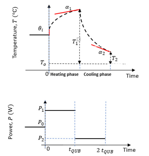
Figure 1.
QUB (Quick U-Value Building) test method and steps.
In QUB test method, the overall heat loss coefficient is estimated as [16]:
where:
| slope of the measured indoor temperature at the end of heating phase; | |
| slope of measured indoor temperature at the end of cooling phase; | |
| input power during heating phase, W; | |
| input power during cooling phase, W; | |
| temperature difference between indoor and outdoor temperature at the end of heating phase, K or °C. | |
| temperature difference between indoor and outdoor temperature at the end of cooling phase, K or °C. |
The outdoor temperature is estimated by taking the mean temperature during the night [17].
Ideal Conditions for QUB Experiment
QUB method is based on the evolution of indoor temperature derived from the differential equation [15]:
where:
| apparent heat capacity or thermal mass of the building, J/K; | |
| indoor air temperature, K or °C; | |
| power input during heating phase, W; | |
| ambient/outdoor temperature, K or °C. | |
| overall heat loss coefficient, W/K |
The conditions for the derivation of QUB Equation (4) from Equation (5) are that the outdoor temperature should remain constant during heating and cooling phases [18]. A steady setpoint temperature is maintained before the experiment [14]. The power dissipated during the cooling phase should be zero, i.e., . The method assumes that homogeneous internal temperature is maintained inside the building; in case of a house with many rooms, the temperature during heating and cooling phases inside each room should be ideally the same, a condition that is difficult to achieve in real experiments. There should be no air stratification (temperature difference along the height of the room) inside the zones. There are different techniques used to avoid stratification of air, i.e., using mat-heaters in vertical position for heating, fans for mixing of indoor air, or taking temperatures at different levels/heights and then taking the mean indoor temperature for QUB estimations. The test is carried with no occupants inside [8].
Ideally, QUB experiment should start from the steady-state conditions. The literature, however, does not mention how long before QUB test an initial steady state should be maintained [13].
The temperature evolution during QUB experiment depends on the initial internal air temperature as well as the distribution of different temperatures inside the building envelope. Before the start of QUB experiment, the building should be in steady state [16]. The power input is from an electric heater as the heating from gas or boiler requires conversion efficiencies for power calculation that can increase the errors.
To reduce the variance of QUB results, a dimensionless quantity is introduced [16]:
where is the assumed initial power before the start of QUB experiment and is given as [15]:
where is the temperature difference between initial indoor temperature and the average outdoor temperature during the night. Since in Equation (2) is not known in advance of QUB experiment, it can be determined from either the design value or from calculations using envelope surface properties [10]. The power should be optimized based on the value of [14]. The heating and cooling phases should be of equal durations. The theoretical model shows a strong dependence on value. For experiments, it is recommended that should be between 0.4 and 0.7 [14].
The ideal conditions for QUB experiment, as discussed in this section, can be summarized as [19]:
- -
- constant outdoor temperature during the experiment;
- -
- homogenous temperature inside the zone where the experiment is performed;
- -
- building should be in steady-state conditions before the start of QUB experiment;
- -
- equal duration of heating and cooling phases;
- -
- power ratio (Equation (6)) between 0.4 to 0.7.
The robustness of QUB method was tested by both numerical and physical experiments. QUB experiments were carried out in a house with controlled environment, in a detached house, and an apartment with real weather conditions [8,13,14,16]. The results of these experiments show that QUB method can generate results within ±15% of the reference overall heat loss coefficient () (obtained via co-heating experiment). The simulation of QUB experiments for non-ideal weather conditions and a well-insulated house (large temperature variation during the experiment night) show that results lie within of the reference [10].
A method for the design of experiment by simulation was developed in which the error can be predicted for any power and time duration [17]. It was shown that QUB experiment can be performed with duration of time shorter than the second-largest time constant of the building and that QUB method is robust at the variation of the optimum power during the heating phase [10,17]. The method shows also robustness with variation in the insulation level of the building for which the experiment was originally designed such that even with error in overall heat loss coefficient, the QUB errors lie within of the reference value [10].
The robustness of QUB experiment was tested on a real house [7]. The indoor temperature was maintained at steady-state value using thermostatically controlled heaters. The house was tested between the end of September and the end of April. The experiment reported that errors for QUB test were within of the steady-state value of the overall heat transfer coefficient. There was no influence of criterion on the results, provided that the -value was maintained in the range of [7]. When , the results were consistently within region. The results of the experiments performed on a real house showed that there is no correlation between the wind speed and -value of the QUB method, although it was argued that the house was sheltered from three sides and only the west side of the house was exposed [7]. The QUB experiments for an apartment building showed that results were in good agreement with steady-state test method. Some of the variance (with a determination coefficient of 0.21 to 0.16) in QUB results can be attributed to external temperature, where an increased external temperature can increase the -value measured with QUB method [8].
QUB experiments show relative robustness, as discussed in literature [16,18,19,20]. However, there is a limited experiment set that discusses the variation of QUB results with change in test conditions and insulation levels of building. The performance of the method when ideal conditions are not respected during the experiment needs to be analyzed further [14]. In the knowledge of authors, influence of different seasons such as summer or winter was not tested. This work aims to simulate QUB experiments under non-ideal conditions during the experiment. QUB experiments are simulated for winter and summer seasons to analyze the suitability of particular season for QUB experiments. Experiments are simulated using different levels of insulation to determine the effectiveness of QUB method with building typologies.
2. Model Description and Validation
In order to simulate QUB experiments under non-ideal conditions, a dynamic state-space model is used to perform the simulations [21]. The dynamic simulations are based on the Heat Balance method of ASHRAE [22] using hour-by-hour typical EnergyPlus meteorological data file [23] interpolated to obtain a timestep of 10 min. The model is generated in the steps: description of building components, generation of thermal circuits, assembling of thermal circuits, conversion of assembled circuits to state-space model, and numerical simulation of the model with weather and indoor power data [21]. The method has the advantage of obtaining the model of the building as a single matrix. This allows us to obtain the eigenvalues and time constants of the building that can be used to analyze QUB method. The state-space modeling method also offers a transparent way of running the simulations, controlling the time step for simulation, changing the geometry of buildings, and changing layers and components of the envelope. The weather data can be manipulated conveniently to determine the influence of boundary conditions, such as solar radiations, outdoor temperature, etc. [10].
A model calibrated on a real house is used to simulate QUB experiments. The house consists of attic, ground floor, and basement [24]. The ground floor of the house is used for QUB experiments. The ground floor is enclosed on the top by an attic and on the bottom by a basement. Therefore, the soil and roof heat exchange is not considered in this study. The ground floor consists of seven zones: kitchen, doorway, two bedrooms, bathroom, corridor, and living room (Figure 2). The blinds on southern face are kept closed to reduce the influence of solar radiation. The outdoor ventilation system in the house is closed during the experiments.
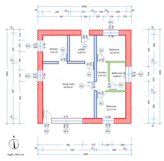
Figure 2.
The twin house layout and dimensions (centimeters).
In addition to the experiments conducted in IEA Annex 58 [24], QUB experiments were performed in this house for 15 days during the spring of 2014 [14]. The cellar was kept at constant temperature of 20 °C to reduce the heat flow. QUB experiment was performed fifteen minutes after the sunset every day. Heating was done with floor mats of 115 W in vertical position to avoid air stratification; the ventilation system was turned on to further improve the temperature homogeneity of the air in the rooms [14].
The experimental data from QUB experiments were used to validate the simulation model used for numerical QUB experiments (Figure 3). The cellar and the attic zones were considered as boundary conditions. It can be observed that the simulation model (kitchen zone) follows the measured temperature within ±0.5 °C (Figure 3). The increased errors on days 5 and 6 are due to the missing temperature data.
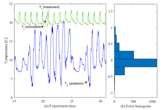
Figure 3.
QUB experiments (a) simulated temperature (red line) comparison with measured temperature (green line) and outdoor temperature (blue line). (b) Simulation error histogram.
The purpose of this work is to analyze the accuracy of QUB method with changing indoor and outdoor conditions. The analysis is performed by simulating QUB experiments using the construction data of the twin house (Figure 2) and recorded weather data [24]. The experiments are performed by simulating the evolution of indoor temperature during the heating and cooling phases of QUB experiment with the weather conditions of the outdoor environment. An overall heat transfer coefficient obtained using steady-state method is used as benchmark for comparison with QUB experiments. Assuming that the height of each zone is the same, the steady-state overall heat transfer coefficient is [17]:
where:
| power supplied to each zone/room of the twin house, W; | |
| surface area of each room, ; | |
| temperature of each room, °C; | |
| outdoor temperature, °C. |
To estimate the steady-state overall heat transfer coefficient, a numerical experiment is designed by applying heating power to control the indoor air at a given setpoint temperature in steady-state conditions. The indoor air temperature and the required heating power for each zone are measured during the simulation. The overall heat transfer is then estimated using Equation (3) with heating power, temperature of each zone, and outdoor temperature as inputs. The overall heat transfer coefficient estimated in this case was 90 .
3. Empirical Analysis of the Influence of Non-Ideal Conditions
3.1. Influence of Variation Outdoor Temperature during QUB Night
The derivation of QUB experiments assumes that the external temperature is constant during heating and cooling phases [14]. This condition may not be respected in real experiments where the temperature can vary during both phases. The outdoor temperature variation and the assumed constant outdoor during a typical QUB night are shown in (Figure 4).
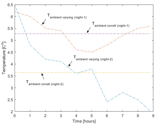
Figure 4.
Temperature variation during a typical night for QUB experiment; horizontal dashed line shows the assumed constant temperature during QUB night.
It is interesting to find the impact of variation of outdoor temperature on QUB results when the perfect conditions of constant outdoor temperature are not respected during the test. Two sets of QUB experiments are performed for winter months starting from November to end of March (150 days) for the weather data of Munich, Germany. One set of experiments is performed with constant outdoor temperature and the other set is performed with varying outdoor temperature during QUB experiments.
Figure 5 shows the results when the QUB experiments are performed:
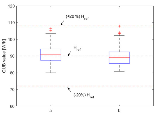
Figure 5.
Comparison between QUB results at: (a) varying outdoor temperature; (b) constant outdoor temperature. The black dashed line shows the steady-state overall heat transfer coefficient and the two red dashed lines show of the steady-state overall heat transfer coefficient.
- at the real outdoor temperature with normal variation during QUB night;
- at the assumed constant outdoor temperature by taking the average outdoor temperature during the experiment night.
The results of QUB experiments for both conditions (a) and (b) lie within of the steady-state overall heat transfer coefficient. Figure 5 shows that, with both constant and variable outdoor temperatures, QUB results are relatively similar.
3.2. Influence of Change in Building Envelope State/Temperature
QUB experiment can be designed if a simulation model is available [17]. For any simulation model to accurately predict the error in QUB experiment, the initial conditions (i.e., the values of the temperature in the walls of the building) need to be correctly defined. The inability to realize the true states of the building envelope can lead to erroneous predictions. The error curves in Figure 6 are generated for the same house at the same outdoor temperature and power levels during QUB experiment. However, the initial states, i.e., the initial temperature of the surfaces and layers of building, were different during each simulation. The different initial states are generated by changing the temperature of the building wall layers before the start of the simulation of QUB experiment.
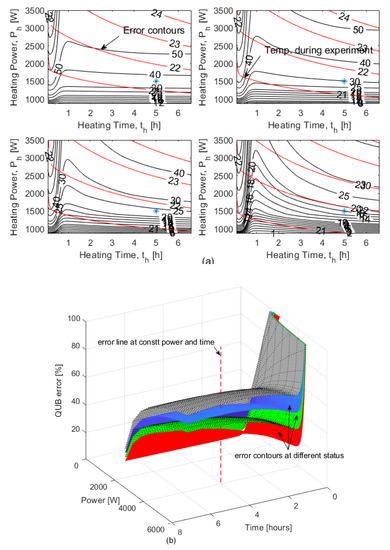
Figure 6.
(a) Four QUB experiments performed at different initial states but same time duration (5 h) and power (1500 W). Blue asterisks show the error of QUB experiment at the given time and power (i) top left panel 35% error, (ii) top right panel 30% error, (iii) bottom left panel 24% error and (iv) bottom right panel 12% error. The black lines are constant error contour lines and red lines the maximum indoor temperature achieved during the QUB experiment. The blue asterisk shows the error (b) The same experiments as in (a) but with error curves shown in 3D (errors shown by the red vertical line).
The results of simulation show that, with the changed states, QUB error also changes (Figure 6a). The error curves in Figure 6b are generated for the same building but with different temperature/states of building envelope; the red dashed line shows that an experiment at the same power, outdoor temperature, and time duration will result in different errors. A design of experiment, therefore, may not be relied upon if the real states of the building are not taken into account during QUB experiment. This also helps us understand that with the changed states, every time a QUB experiment is repeated, the results can be different.
3.3. Influence of Meteorological Conditions
The variation of meteorological conditions during QUB experiment can change the results. The design of QUB experiment depends on the predicted temperature during the experiment. It is expected that outdoor conditions can deviate from the predicted weather conditions. The effects of meteorological uncertainties can be reduced by performing QUB experiment at higher level of power [21]. To analyze the effect of the meteorological uncertainty, a QUB experiment was simulated at power level of 5000 W during the heating phase. The experiment was simulated at the predicted average outdoor temperature that was 10 °C in this case. The experiments were then repeated at 8 °C and 12 °C. The rise and fall of temperature during these three experiments are shown in Figure 7. It can be observed that the responses at different outdoor temperatures are only slightly different (Figure 7). The variation in QUB results with the variation of predicted outdoor temperature in this case is in the range of .
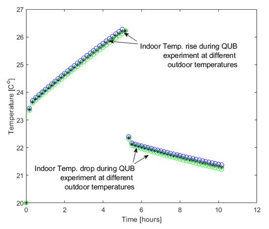
Figure 7.
QUB experiments at different outdoor temperatures: at predicted average outdoor temperature (black asterisks) of 10 °C, at 8 °C (green circles), and at 12 °C (blue circles).
3.4. Influence of Seasons (Winter and Summer)
Since the results of QUB experiment depend on outdoor conditions, QUB experiments were simulated during summer and winter seasons. Hourly weather data for the city of Munich [23] was used to simulate the QUB experiment on a house specified in IEA, EBC Annex-58 [24]. The data were interpolated to generate data at sample time of 10 min. The applied power was optimized using (see Equation (9)) with no power during the cooling phase. Figure 8 shows the results for November to March and for June to August. The heating and cooling phase has a duration of 4.5 h. The results of the experiment show that, in winter season (November to March), QUB experiments have less error and variation. The majority of the results are within of the reference overall heat coefficient (Figure 8, box plot on left).
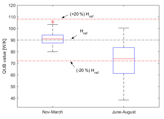
Figure 8.
Errors of QUB experiments performed during winter and summers.
For the summer season (June, July, August), QUB experiments show large variation. The majority of QUB experiments show an underestimation (Figure 8, box plot on right). The set temperature before the start of QUB experiments was maintained at 20 °C during these experiments. It may be mentioned that the majority of the in-situ overall heat transfer coefficient testing methods are recommended for seasons where a minimum temperature difference of 10 K can be maintained between indoor and outdoor temperature, a condition that is difficult to achieve during summer time [3].
The underestimated QUB results during the summer season coincide with high outdoor temperatures during QUB experiments, i.e., a low temperature difference between indoor and outdoor temperatures before the start of QUB experiment.
Figure 9 shows the temperature difference at the time of the beginning of QUB experiments during summer months and QUB error. It is evident that the small temperature difference between outdoor and indoor temperature results in larger errors. It can be seen that with the temperature difference above 10 K, the error remains within . The reason for this is that with a small temperature difference (also due to short duration of QUB method) the perturbation is not enough to provide a good measurement to noise ratio during the QUB experiment. This is in line with the required protocol for test methods such as co-heating and ISABELE, where a temperature difference greater than 10 K is recommended [12].
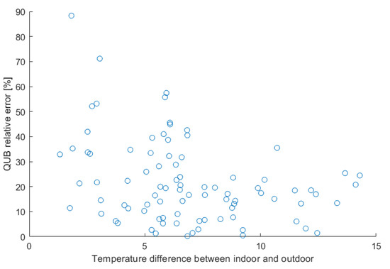
Figure 9.
QUB error as a function of difference between outdoor and indoor temperature before the start of experiment.
It can be concluded that winter is a better season for QUB experiment. In summer, the variation and error in QUB experiment are relatively large due to small temperature difference between indoor and outdoor temperatures.
The large errors during summer can be understood with respect to the optimum power during the heating phase of a QUB experiment, which can be given by the -criterion [15]:
where is computed as . An acceptable range for should be between 0.5 and 0.7 [15]. The heating power , therefore, can be given as:
where should be between 2 and 4 for to be between 0.5 and 0.7. During summer, the temperature difference between indoor (set at 20 °C) and outdoor is small. During summer days, with the temperature difference smaller than 10 K, experiments with , i.e., in equation (5) results in a small power during heating phase, producing an underestimation of overall heat transfer coefficient as shown in Figure 8 (box plot for summer).
In order to increase the temperature difference in summer, QUB experiments were repeated with a higher setpoint temperature of 25 °C before the start of the experiment. The experiments show that, at high indoor set temperature, the results of QUB experiment improve (Figure 10). The majority of QUB results are within of the steady-state overall heat transfer coefficient, with few outliers. The results are further improved by increasing the power ratio (). An increase in power ratio above 0.7 results in overestimation of QUB results.
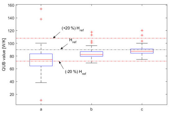
Figure 10.
QUB experiments when simulated at (a) 20 °C setpoint temperature and ( ), (b) 25 °C setpoint temperature and (n = 2) (c) 25 °C setpoint temperature and (n = 3).
3.5. Optimum Power for Winter
To determine the optimum power for winter, a number of experiments were performed from November to March at different levels of heating power with ranging from 2 to 6. The results can be viewed in Table 1. It can be observed that with between 2 and 3, QUB results are closer to the steady-state overall heat transfer coefficient. It must be mentioned that the value of is valid for a temperature difference that is above 10 K. The extreme outdoor conditions, such as an extremely cold outdoor temperature, can lead to high power, even with lower than 2.

Table 1.
QUB experiment during winter months at different levels of power.
3.6. QUB Experiments for Buildings with Lower Overall Heat Transfer Coefficient
QUB experiments presented above were simulated for a house that has relatively high level of insulation with an overall heat transfer coefficient value of 90 W/K. In order to determine the behavior of QUB method for buildings with low level of insulation, QUB experiments were simulated for the same house but with the overall heat transfer coefficient of 134 W/K and 179 W/K. Experiments were simulated for one year. It can be inferred from results shown in Table 2 that, with the reduced insulation, the median error for the QUB experiments is reduced.
Table 2.
QUB experiments at different insulation level of building.
4. Conclusions
This work discusses the ideal conditions for QUB test and then simulates QUB experiments for a real house in non-ideal weather conditions. The model used to simulate QUB experiments is validated using International Energy Agency—Energy in Buildings and Communities (IEA-EBC) Annex 58 data set along with real QUB experiments conducted in the same house. Weather data for Munich is used to simulate QUB experiments for the ground floor of the house. The results of simulation experiments can be concluded as follows:
- QUB experiments were simulated with variable and constant outdoor temperature during the night. Majority of the errors for variable and constant outdoor temperature (during QUB experiment) lie within . The variation of QUB results for variable and constant outdoor temperature was relatively similar.
- The simulation results of QUB experiment can vary with the initial conditions of the building envelope. The reason QUB experiments show variations when repeated is that between two experiments the temperature inside the building envelope cannot remain the same.
- The meteorological conditions for which QUB experiment is designed may vary, i.e. the outdoor temperature can increase or decrease during QUB night. For a temperature difference between indoor and outdoor of 10 K, a variation of 2 K in outdoor temperature changes QUB results within .
- A comparison of QUB experiments for summer and winter shows that the winter season can be considered more suitable for QUB experiments. Experiments conducted for the month of November, December, January, February, and March show that the majority of the errors lie within with few outliers around .
- QUB experiments for summer months (June, July, and August) show large variation (errors). However, it is possible to predict the experiment outcome by observing the difference between indoor temperature and outdoor temperature during QUB experiment.
- The experiments during summer give large errors when the temperature difference between the initial indoor and outdoor temperature is smaller than 10 K. With setpoint of 20 °C, the difference between indoor and outdoor temperature for few days remained smaller than 10 K. The experiments in such conditions generated large errors.
- The results during summer days were improved by using a high setpoint temperature (25 °C), such that the majority of the errors remained within ±20 °C of the steady-state overall heat transfer coefficient. The summer results can be further improved by using a higher power ratio, i.e., .
- QUB experiments for winter show results close to steady-state overall heat transfer coefficient when -value (power ratio) is between 0.5 and 0.7.
- The performance of QUB method shows that the method can respond well for buildings with reduced insulation.
Author Contributions
Conceptualization, C.G.; data curation, M.Q.; formal analysis, C.G.; investigation, N.A.; methodology, N.A. and C.G.; project administration, C.G.; software, N.A.; supervision, C.G.; validation, M.Q.; writing—original draft, N.A.; writing—review and editing, C.G. and M.Q. All authors have read and agreed to the published version of the manuscript.
Funding
This research was partly funded by Campus France and Higher Education Commission (HEC), Pakistan (80%), through a doctoral scholarship awarded to Naveed Ahmad and partly (20%) by Saint Gobain, through a research contract.
Acknowledgments
The description of the building and the experimental data were provided by Fraunhofer-Institut für Bauphysik IBP, Holzkirchen, 83626 Valley, Germany. The support of Paul Strachan from Energy Systems Research Unit, University of Strathclyde, Glasgow, G1 1XJ, UK, and Ingo Heusler and Matthias Kersken from Fraunhofer-Institut für Bauphysik IBP, Holzkirchen, 83626 Valley, Germany are highly appreciated. The continuous inputs and recommendations of Thimothee Thiery, Research Engineer at Saint Gobain, are highly appreciated.
Conflicts of Interest
The authors declare no conflict of interest.
Nomenclature
| surface area, m2 | |
| thermal capacity, J/K | |
| solar radiation received by the building (absorbed and transmitted), W/m2 | |
| steady-state overall heat loss coefficient (HLC), W/K | |
| reference/steady-state overall heat loss coefficient, W/K | |
| overall heat loss coefficient measured using QUB method, W/K | |
| power measured before the beginning of QUB experiment, W | |
| power measured during the heating phase of QUB experiment, W | |
| power measured during the cooling phase of QUB experiment, W | |
| temperature, K or °C | |
| outdoor temperature, K or °C | |
| indoor temperature, K or °C | |
| temperature difference between outside and inside air during the heating phase, K or °C | |
| temperature difference between outside and inside air during the cooling phase, K or °C | |
| heat transfer coefficient, W/(m2 K) | |
| Greek letters | |
| mean (or equivalent) temperature, K or °C | |
| indoor temperature, K or °C | |
| time constant, hour or seconds | |
| heat input, W | |
| temperature slope during heating phase of QUB experiment | |
| temperature slope during cooling phase of QUB experiment | |
References
- Lucon, O.; Hashem, A.; Bertoldi, P.; Cabeza, L.F.; Eyre, N.; Gadgil, A.; Harvey, L.D.D.; Jiang, Y.; Liphoto, E.; Mirasgedis, S.; et al. Buildings. In Climate Change: Climate Change Mitigation; Contribution of Working Group III to Fifth Assessment Report of the Intergovernmental Panel on Climate Change; Intergovernmental Panel on Climate Change: Geneva, Switzerland, 2014; Volume 33, pp. 1–66. [Google Scholar]
- Energy Information Administration-EIA-Official Energy Statistics from the U.S. Government EIA-“International Energy Outlook 2019”. Retrieved from Official Website of US Energy Information Administration. Available online: www.eia.gov/outlooks/ieo/pdf/ieo2019.pdf (accessed on 20 June 2020).
- Bauwens, G.; Roels, S. Co-heating test: A state-of-the-art. Energy Build. 2014, 82, 163–172. [Google Scholar] [CrossRef]
- Demanuele, C.; Tweddell, T.; Davies, M. Bridging the gap between predicted and actual energy performance in schools. In Proceedings of the World Energy Congress XI, Abu Dhabi, UAE, 23–25 September 2010. [Google Scholar]
- Rasooli, A.; Itard, L.; Ferreira, C.I. A response factor-based method for the rapid in-situ determination of wall’s thermal resistance in existing buildings. Energy Build 2016, 119, 51–61. [Google Scholar] [CrossRef]
- Brun, A.; Alzetto, F.; Boisson, P.; Thebault, S. Short methodologies for in-situ assessment of the intrisinc thermal performance of the building envelope. In Proceedings of the Sustainable Places, Nice, France, 1–3 October 2014. [Google Scholar]
- Sougkakis, V.; Meulemans, J.; Alzetto, F.; Wood, C.; Cox, T. An assessment of the QUB method for predicting the whole building thermal performance under actual operating conditions. In Proceedings of the International SEEDS Conference, Leeds, UK, 13–14 September 2017. [Google Scholar]
- Foucquier, A.; Robert, S.; Suard, F.; Stephan, L.; Jay, A. State of the art in building modelling and energy performances prediction: A review. Renew. Sustain. Energy Rev. 2013, 23, 272–288. [Google Scholar] [CrossRef]
- Stamp, S.; Altamirano-Medina, H.; Lowe, R. Assessing the Relationship between Measurement Length and Accuracy within Steady State Co-Heating Tests. Buildings 2017, 7, 98. [Google Scholar] [CrossRef]
- Ahmad, N.; Ghiaus, C.; Thiery, T. Influence of Initial and Boundary Conditions on the Accuracy of the QUB Method to Determine the Overall Heat Loss Coefficient of a Building. Energies 2020, 13, 284. [Google Scholar] [CrossRef]
- Subbarao, K. PSTAR: Primary and Secondary Terms Analysis and Renormalization: A Unified Approach to Building Energy Simulations and Short-Term Monitoring; Report SERI/TR-254-3347; Solar Energy Research Institute: Golden, CO, USA, 1988. [Google Scholar]
- Boisson, P.; Bouchié, R. ISABELE method: In-situ assessment of the building envelope performances. In Proceedings of the Ninth International Conference on System Simulation Building, Liege, Belgium, 1 December 2014; pp. 1–20. [Google Scholar]
- Pandraud, G.; Didier, G.; Alzetto, F. Experimental optimization of the QUB method, In IEA EBC Annex 58. In Proceedings of the 6th Expert meeting, Ghent, Belgium, 14–16 April 2014. [Google Scholar]
- Alzetto, F.; Pandraud, G.; Fitton, R. QUB: A fast dynamic method for in-situ measurement of the whole building heat loss. Energy Build. 2018, 174, 124–133. [Google Scholar] [CrossRef]
- Meulemans, J.; Alzetto, F.; Farmer, D.; Gorse, C. QUB/e: A novel transient experimental method for in situ measurements of the thermal performance of building fabrics. In Proceedings of the International Sustainable Ecological Engineering Design for Society (SEEDS) Conference, Leeds, UK, 14–15 September 2016. hal-01589176. [Google Scholar]
- Alzetto, F.; Farmer, D.; Fitton, R.; Hughes, T.; Swan, W. Comparison of whole house heat loss test methods under controlled conditions in six distinct retrofit scenarios. Energy Build. 2018, 168, 35–41. [Google Scholar] [CrossRef]
- Ghiaus, C.; Alzetto, F. Design of experiments for Quick U-building method for building energy performance measurement. J. Energy Build. Perform. Simul. 2019. [Google Scholar] [CrossRef]
- Meulemans, J. An assessment of the QUB/e method for fast in situ measurements of the thermal performance of building fabrics in cold climates, in Cold Climate HVAC 2018. In Proceedings of the 9th International Cold Climate Conference, Lund University, Kiruna Sweeden, 12–15 March 2018. hal-01737563. [Google Scholar]
- Meulemans, J.; Alzetto, F.; Farmer, D.; Gorse, C. QUB/e: A Novel Transient Experimental Method for in situ Measurements of the Thermal Performance of Building Fabrics. In Building Information Modelling, Building Performance, Design and Smart Construction; Springer International Publishing: Cham, Switzerland, 2017; pp. 115–127. [Google Scholar]
- Alzetto, F.; Meulemans, J.; Pandraud, G.; Roux, D. A perturbation method to estimate building thermal performance. Comptes Rendus Chim. 2018, 21, 938–942. [Google Scholar] [CrossRef]
- Ghiaus, C.; Ahmad, N. Thermal circuits assembling and state-space extraction for modelling heat transfer in buildings. Energy 2020, 195, 117019. [Google Scholar] [CrossRef]
- Bellenger, L.; Bruning, S.; Pedersen, C.; Romine, T.; Wilkins, C. Nonresidential Cooling and Heating Load Calculation Procedures. In ASHRAE Handbook: Fundamentals; ASHRAE: Atlanta, GA, USA, 2001; ISBN 10: 1931862516. [Google Scholar]
- Weather Data | EnergyPlus. Available online: https://energyplus.net/weather (accessed on 2 April 2020).
- Strachan, P.; Heusler, I.; Kersken, M.; Jiménez, M.J. Empirical Whole Model Validation Modelling Specification Validation of Building Energy Simulation Tools. J. Build. Perform. Simul. 2016, 9, 331–350. [Google Scholar] [CrossRef]


© 2020 by the authors. Licensee MDPI, Basel, Switzerland. This article is an open access article distributed under the terms and conditions of the Creative Commons Attribution (CC BY) license (http://creativecommons.org/licenses/by/4.0/).