Eulerian Two-Fluid Model of Alkaline Water Electrolysis for Hydrogen Production

 ,
,  ,
,  , and
, and 
Abstract
:1. Introduction
2. Numerical Methods
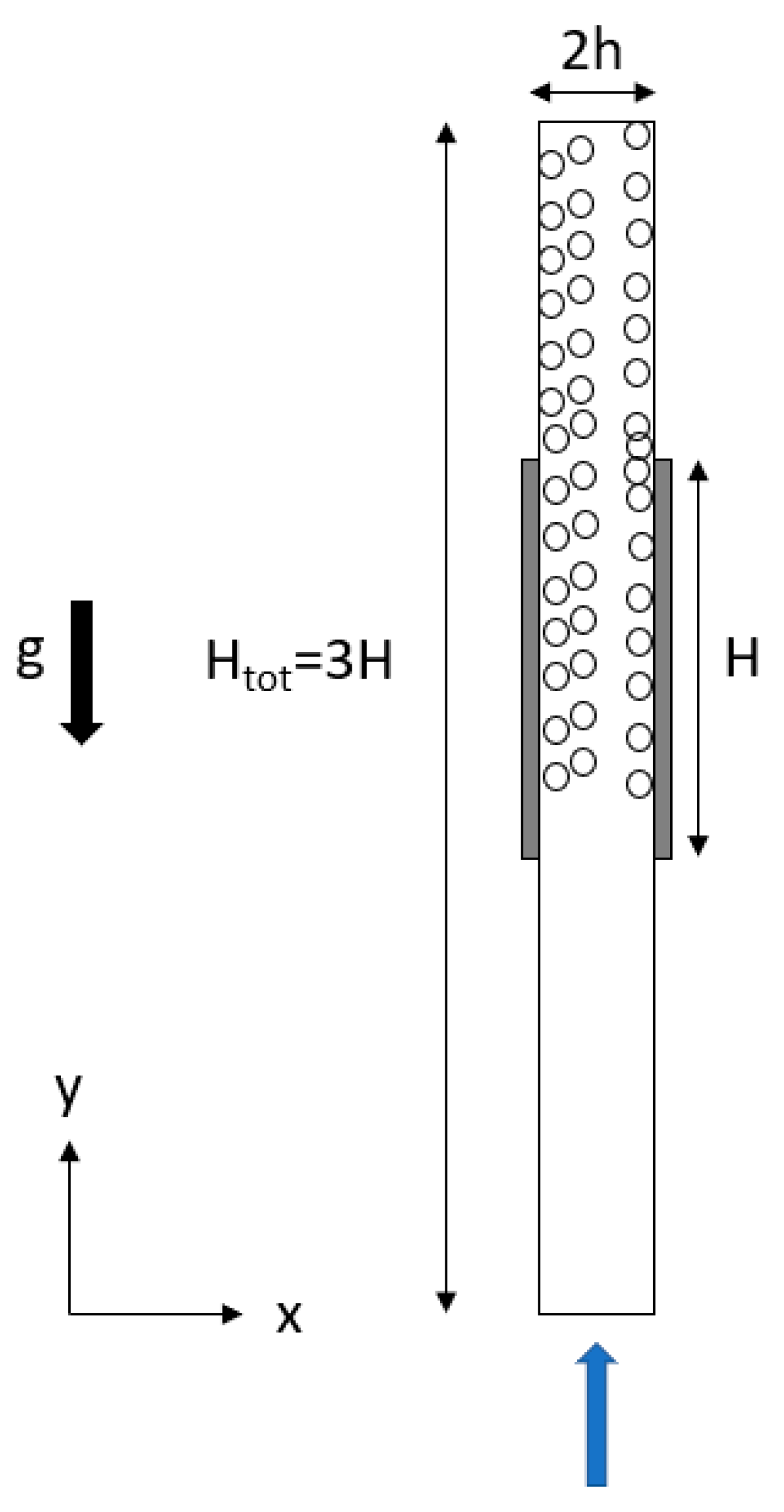
2.1. Geometry and Mesh
2.2. Mathematical Formulation
2.2.1. The Bubble Dispersion Problem
2.2.2. Model
- The flow is Newtonian, viscous and incompressible;
- Due to the high heat transfer induced by the bubbles and the relatively low surface and volume inducing a low heat injection by ohmic and activation losses, the flow is considered isothermal
- At the same time, numerical simulations were carried out in order to highlight the influence of ions on the velocity and void fraction distribution. There were only very little differences when the ions distribution was taking into account. Thus, the electrolyte is considered as extremely well mixed. This hypothesis has been made also by Abdelouahed et al. [26] and Schillings et al. [14];
- Oxygen, hydrogen and electrolytes are three continuum media;
- Because the Reynolds number calculated via the data from Boissonneau et al. [15] is between 240 and 480, the flow is considered as laminar;
- The effect of the surface tension is neglected;
- Nagai et al. [28] observed a dependency of the diameter with respect with the current density and in addition to this dependency, Boissonneau et al. [15] observed that the bubble diameter increases with height. Schillings et al. [14] chose to make the diameter increase with the height and current density. In the current study and in other studies [12,13], it was decided that a constant bubble diameter is taken for a given current density. Although this hypothesis is made in a lot of studies, it does not reflect the reality. There is a distribution of the bubble diameter, but since it is not yet possible to model this distribution, we are forced to make this assumption;
2.3. Boundary Conditions
2.4. Numerical Procedure
3. Results
4. Conclusions
Author Contributions
Funding
Acknowledgments
Conflicts of Interest
References
- Castagnola, L.; Lomonaco, G.; Marotta, R. Nuclear Systems for Hydrogen Production: State of Art and Perspectives in Transport Sector. Glob. J. Energy Technol. Res. Updates 2014, 1, 4–18. [Google Scholar]
- Schäfer, H.; Chatenet, M. Steel: The Resurrection of a Forgotten Water-Splitting Catalyst. ACS Energy Lett. 2018, 3, 574–591. [Google Scholar] [CrossRef]
- Lavorante, M.J.; Franco, J.I. Performance of stainless steel 316L electrodes with modified surface to be use in alkaline water electrolyzers. Int. J. Hydrogen Energy 2016, 41, 9731–9737. [Google Scholar] [CrossRef]
- Bocca, C.; Cerisola, G.; Barbucci, A.; Magnone, E. Oxygen evolution on Co2O3 and Li-doped Co2O3 coated electrodes in an alkaline solution. Int. J. Hydrogen Energy 1999, 24, 699–707. [Google Scholar] [CrossRef]
- Boggs, B.K.; King, R.L.; Botte, G.G. Urea electrolysis: Direct hydrogen production from urine. Chem. Commun. 2009, 32, 4859–4861. [Google Scholar] [CrossRef] [PubMed]
- Huck, M.; Ring, L.; Küpper, K.; Klare, J.P.; Daum, D.; Schäfer, H. Water Splitting Mediated by an Electrocatalytically Driven Cyclic Process Involving Iron Oxide Species; Huck, Marten, Lisa Ring, Karsten Küpper, Johann Klare, Diemo Daum, and Helmut Schäfer. J. Mater. Chem. A 2020, 8, 9896–9910. [Google Scholar] [CrossRef]
- Babu, R.; Das, M.K. Experimental studies of natural convective mass transfer in a water-splitting system. Int. J. Hydrogon Energy 2019, 44, 14467–14480. [Google Scholar] [CrossRef]
- Tobias, C.W. Effect of Gas Evolution on Current Distribution and Ohmic Resistance in Electrolyzers. J. Electrochem. Soc. 1959, 106, 6. [Google Scholar] [CrossRef]
- Hine, F. Bubble Effects on the Solution IR Drop in a Vertical Electrolyzer Under Free and Forced Convection. J. Electrochem. Soc. 1980, 127, 292. [Google Scholar] [CrossRef]
- Mandin, P.; Hamburger, J.; Bessou, S.; Picard, G. Modelling and calculation of the current density distribution evolution at vertical gas-evolving electrodes. Electrochim. Acta 2005, 51, 1140–1156. [Google Scholar] [CrossRef]
- Hreiz, R.; Abdelouahed, L.; Fünfschilling, D.; Lapicque, F. Electrogenerated bubbles induced convection in narrow vertical cells: PIV measurements and Euler–Lagrange CFD simulation. Chem. Eng. Sci. 2015, 134, 138–152. [Google Scholar] [CrossRef]
- Dahlkild, A.A. Modelling the two-phase flow and current distribution along a vertical gas-evolving electrode. J. Fluid Mech. 2001, 428, 249–272. [Google Scholar] [CrossRef]
- Wedin, R.; Dahlkild, A.A. On the Transport of Small Bubbles under Developing Channel Flow in a Buoyant Gas-Evolving Electrochemical Cell. Ind. Eng. Chem. Res. 2001, 40, 5228–5233. [Google Scholar] [CrossRef]
- Schillings, J.; Doche, O.; Deseure, J. Modeling of electrochemically generated bubbly flow under buoyancy-driven and forced convection. Int. J. Heat Mass Transf. 2015, 85, 292–299. [Google Scholar] [CrossRef]
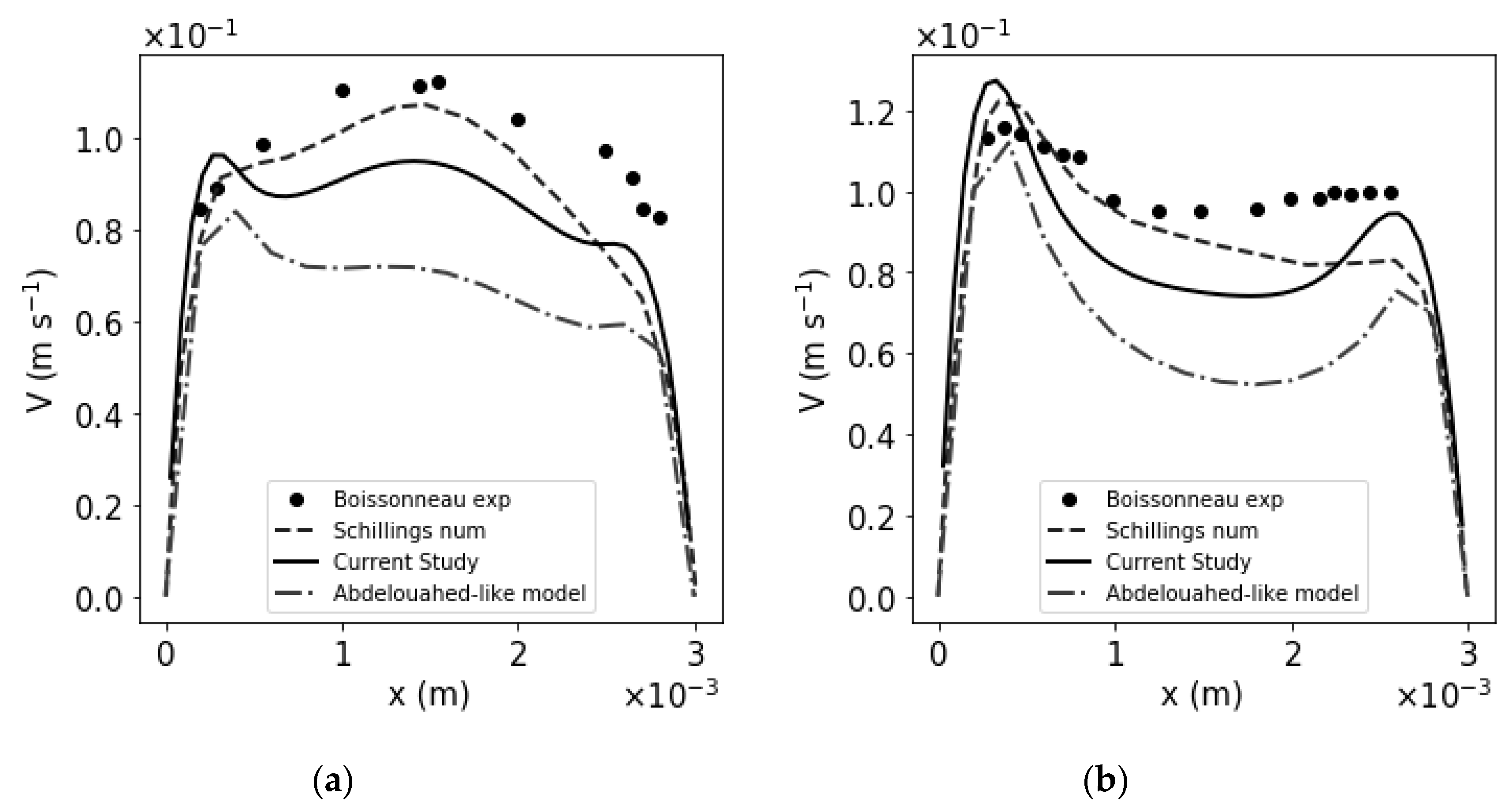
- Boissonneau, P.; Byrne, P. An experimental investigation of bubble-induced free convection in a small electrochemical cell. J. Appl. Electrochem. 2000, 30, 767–775. [Google Scholar] [CrossRef]
- Aldas, K.; Pehlivanoglu, N.; Mat, M.D. Numerical and experimental investigation of two-phase flow in an electrochemical cell. Int. J. Hydrogen Energy 2008, 33, 3668–3675. [Google Scholar] [CrossRef]
- Mat, M. A two-phase flow model for hydrogen evolution in an electrochemical cell. Int. J. Hydrogen Energy 2004, 29, 1015–1023. [Google Scholar] [CrossRef]
- Riegel, H.; Mitrovic, J.; Stephan, K. Role of mass transfer on hydrogen evolution in aqueous media. J. Appl. Phys. 1998, 28, 10–17. [Google Scholar]
- Picardi, R.; Zhao, L.; Battaglia, F. On the Ideal Grid Resolution for Two-Dimensional Eulerian Modeling of Gas–Liquid Flows. J. Fluids Eng. 2016, 138, 114503. [Google Scholar] [CrossRef]
- Law, D.; Battaglia, F.; Heindel, T.J. Model validation for low and high superficial gas velocity bubble column flows. Chem. Eng. Sci. 2008, 63, 4605–4616. [Google Scholar] [CrossRef]
- Panicker, N.; Passalacqua, A.; Fox, R.O. On the hyperbolicity of the two-fluid model for gas—Liquid bubbly flows. Appl. Math. Model. 2018, 57, 432–447. [Google Scholar] [CrossRef] [Green Version]
- Vaidheeswaran, A.; de Bertodano, M.L. Stability and convergence of computational eulerian two-fluid model for a bubble plume. Chem. Eng. Sci. 2017, 160, 210–226. [Google Scholar] [CrossRef]
- Marfaing, O.; Guingo, M.; Laviéville, J.; Bois, G.; Méchitoua, N.; Mérigoux, N.; Mimouni, S. An analytical relation for the void fraction distribution in a fully developed bubbly flow in a vertical pipe. Chem. Eng. Sci. 2016, 152, 579–585. [Google Scholar] [CrossRef] [Green Version]
- Davidson, M.R. Numerical calculations of two-phase flow in a liquid bath with bottom gas injection: The central plume. Appl. Math. Model. 1990, 14, 67–76. [Google Scholar] [CrossRef]
- Lee, J.W.; Sohn, D.K.; Ko, H.S. Study on bubble visualization of gas-evolving electrolysis in forced convective electrolyte. Exp. Fluids 2019, 60, 156. [Google Scholar] [CrossRef]
- Abdelouahed, L.; Hreiz, R.; Poncin, S.; Valentin, G.; Lapicque, F. Hydrodynamics of gas bubbles in the gap of lantern blade electrodes without forced flow of electrolyte: Experiments and CFD modelling. Chem. Eng. Sci. 2014, 111, 255–265. [Google Scholar] [CrossRef]
- Ham, J.; Homsy, G. Hindered settling and hydrodynamic dispersion in quiescent sedimenting suspensions. Int. J. Multiph. Flow 1988, 14, 533–546. [Google Scholar] [CrossRef]
- Nagai, N.; Takeuchi, M.; Nakao, M. Influences of Bubbles between Electrodes onto Efficiency of Alkaline Water Electrolysis. Pac. Cent. Therm. Fluids Eng. 2003, 10, F4008. [Google Scholar]
- Abdelouahed, L. Gestion Optimale du Gaz Électrogénéré Dans un Réacteur D’électroréduction de Minerai de fer. Ph.D. Thesis, Université de Lorraine, Nancy, France, 2013. [Google Scholar]
- Schillings, J. Etude Numérique et Expérimentale D’écoulements Diphasiques: Application aux Écoulements à Bulles Générées par Voie Électrochimique. Ph.D. Thesis, Université Grenoble Alpes, Grenoble, France, 2018. [Google Scholar]
- Le Bideau, D.; Mandin, P.; Sellier, M.; Benbouzid, M.; Myeongsub, K. Review of necessary thermophysical properties and their sensivities with local temperature and electrolyte mass fraction for alkaline water electrolysis multiphysics modelling. Int. J. Hydrogon Energy 2019, 44, 4553–4569. [Google Scholar] [CrossRef]
- Alexiadis, A.; Dudukovic, M.P.; Ramachandran, P.; Cornell, A.; Wanngård, J.; Bokkers, A. Liquid–gas flow patterns in a narrow electrochemical channel. Chem. Eng. Sci. 2011, 66, 2252–2260. [Google Scholar] [CrossRef]
- Alexiadis, A.; Dudukovic, M.P.; Ramachandran, P.; Cornell, A.; Wanngård, J.; Bokkers, A. On the electrode boundary conditions in the simulation of two phase flow in electrochemical cells. Int. J. Hydrogen Energy 2011, 36, 8557–8559. [Google Scholar] [CrossRef]
- Charton, S.; Rivalier, P.; Ode, D.; Morandini, J.; Caire, J.P. Hydrogen Production by the Westinghouse Cycle: Modelling and Optimization of the Two-Phase Electrolysis Cell; WIT Press: Bologna, Italy, 2009; pp. 11–22. [Google Scholar]
- Grigoriev, S.A.; Fateev, V.N.; Bessarabov, D.G.; Millet, P. Current status, research trends, and challenges in water electrolysis science and technology. Int. J. Hydrogon Energy 2020. [Google Scholar] [CrossRef]
- Isono, T. Density, viscosity, and electrolytic conductivity of concentrated aqueous electrolyte solutions at several temperatures. Alkaline-earth chlorides, lanthanum chloride, sodium chloride, sodium nitrate, sodium bromide, potassium nitrate, potassium bromide, and cadmium nitrate. J. Chem. Eng. Data 1984, 29, 45–52. [Google Scholar] [CrossRef]
- Mandin, P.; Derhoumi, Z.; Roustan, H.; Rolf, W. Bubble Over-Potential during Two-Phase Alkaline Water Electrolysis. Electrochim. Acta 2014, 128, 248–258. [Google Scholar] [CrossRef]


| Position | Boundary Conditions |
|---|---|
| x = 0 Helec < y < 2 Helec | |
| x = 2h 0 < y <3 Helec | |
| 0 < x < 2h y = 0 | |
| 0 < x < 2h y = 3 Helec |
| Name | Value |
|---|---|
| Geometry inputs | |
| Helec (mm) | 40 |
| L (mm) | 30 |
| h (mm) | 1.5 |
| HTot (mm) | 120 |
| Physical Inputs | |
| ρl (kg m−3) | 1040 |
| ρO2 (kg m−3) | 1.3 |
| ρH2 (kg m−3) | 0.08 |
| υl (m2 s−1) | 9.97 × 10⁻⁷ |
| Two-Phase Inputs | |
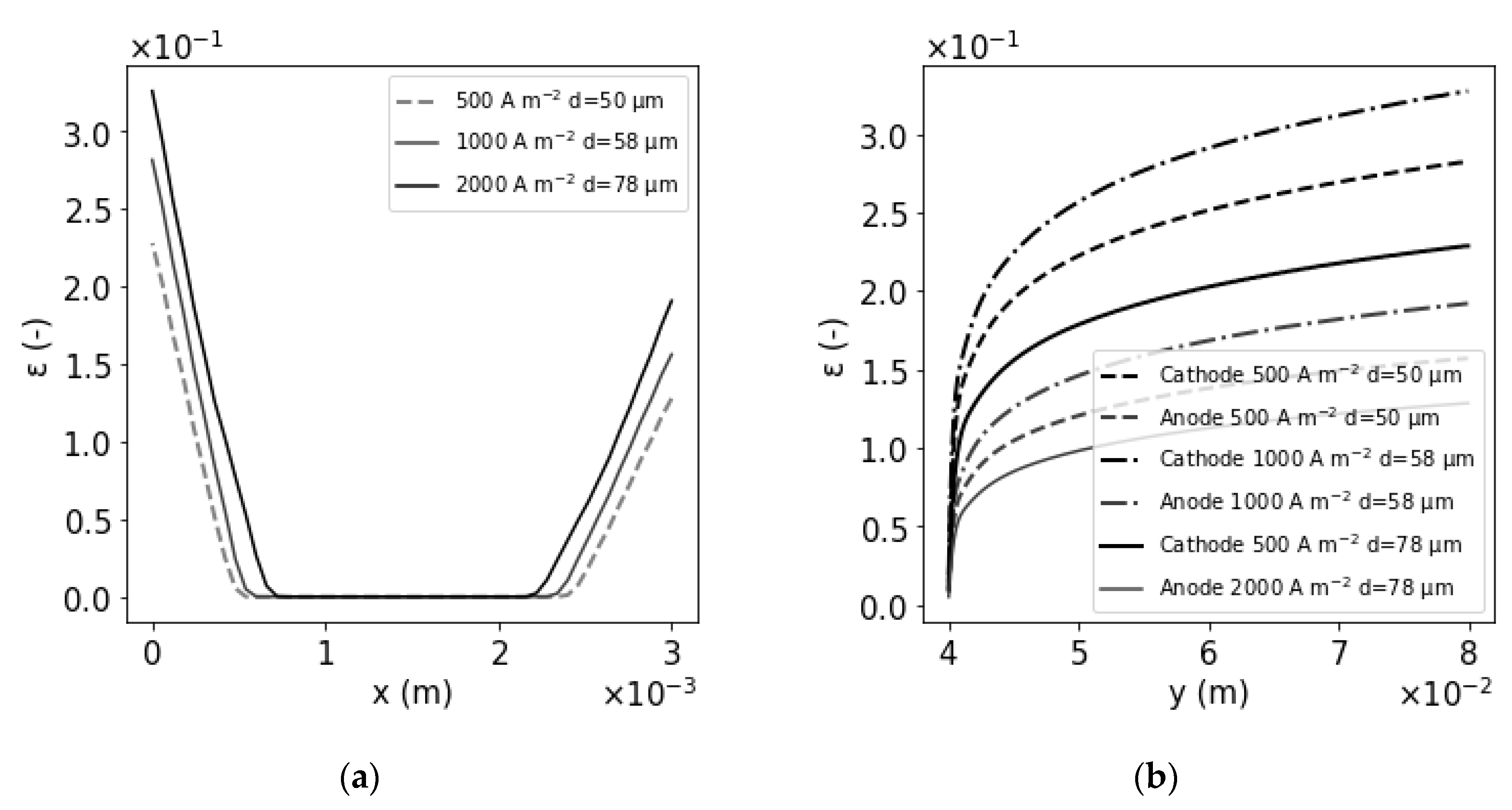
| db (µm) | for 500 A m−2 db = 50 µm for 1000 A m−2 db = 58 µm for 2000 A m−2 db = 78 µm |
| 500 A m−2 | 1000 A m−2 | 2000 A m−2 |
|---|---|---|
| KO2/d = 10.5 | KO2/d = 9 | KO2/d = 5 |
| KH2/d = 5 | KH2/d = 4 | KH2/d = 2.5 |
| j (A m−2) | Model Comparaison | Zone | 60 mm | 75 mm |
|---|---|---|---|---|
| 500 A m−2 | Boissonneau vs. Abdelouahed | H2 | 6.95 × 10⁻² | 3.96 × 10⁻² |
| O2 | 2.48 × 10⁻¹ | 1.47 × 10⁻¹ | ||
| Bulk | 2.91 × 10⁻¹ | 2.91 × 10⁻¹ | ||
| Boissonneau vs. Schillings | H2 | 6.00 × 10⁻² | 1.60 × 10⁻² | |
| O2 | 2.85 × 10⁻¹ | 2.65 × 10⁻¹ | ||
| Bulk | 1.90 × 10⁻¹ | 2.06 × 10⁻¹ | ||
| Boissonneau vs. Current Study | H2 | 1.76 × 10⁻¹ | 4.55 × 10⁻² | |
| O2 | 2.01 × 10⁻¹ | 7.40 × 10⁻² | ||
| Bulk | 2.48 × 10⁻¹ | 2.36 × 10⁻¹ | ||
| 1000 A m−2 | Boissonneau vs. Abdelouahed | H2 | 1.04 × 10⁻¹ | 6.13 × 10⁻² |
| O2 | 3.48 × 10⁻¹ | 2.69 × 10⁻¹ | ||
| Bulk | 3.83 × 10⁻¹ | 3.51 × 10⁻¹ | ||
| Boissonneau vs. Schillings | H2 | 1.21 × 10⁻¹ | 4.76 × 10⁻² | |
| O2 | 2.99 × 10⁻¹ | 2.27 × 10⁻¹ | ||
| Bulk | 1.69 × 10⁻¹ | 1.31 × 10⁻¹ | ||
| Boissonneau vs. Current Study | H2 | 1.04 × 10⁻¹ | 7.95 × 10⁻² | |
| O2 | 2.35 × 10⁻¹ | 6.37 × 10⁻² | ||
| Bulk | 2.50 × 10⁻¹ | 1.99 × 10⁻¹ | ||
| 2000 A m−2 | Boissonneau vs. Abdelouahed | H2 | 1.43 × 10⁻¹ | 7.09 × 10⁻² |
| O2 | 2.69 × 10⁻¹ | 3.58 × 10⁻¹ | ||
| Bulk | 3.51 × 10⁻¹ | 3.70 × 10⁻¹ | ||
| Boissonneau vs. Schillings | H2 | 4.76 × 10⁻² | 4.31 × 10⁻² | |
| O2 | 2.27 × 10⁻¹ | 2.90 × 10⁻¹ | ||
| Bulk | 1.31 × 10⁻¹ | 6.27 × 10⁻² | ||
| Boissonneau vs. Current Study | H2 | 7.95 × 10⁻² | 7.44 × 10⁻² | |
| O2 | 6.37 × 10⁻² | 1.71 × 10⁻¹ | ||
| Bulk | 1.99 × 10⁻¹ | 2.57 × 10⁻¹ |
| j (A m−2) | Vmax liq cath (m s−1) | Vmax liq an (m s−1) | εmax cath | εmax an | δcath (µm) | δan (µm) | R(ε)/R |
|---|---|---|---|---|---|---|---|
| 500 A m−2 | 7.8 × 10⁻² | 4.8 × 10⁻² | 0.23 | 0.13 | 515 | 600 | 1.032 |
| 1000 A m−2 | 9 × 10⁻² | 6.8 × 10⁻² | 0.28 | 0.16 | 566 | 677 | 1.043 |
| 2000 A m−2 | 1.25 × 10⁻¹ | 9.1 × 10⁻² | 0.33 | 0.19 | 690 | 800 | 1.057 |
© 2020 by the authors. Licensee MDPI, Basel, Switzerland. This article is an open access article distributed under the terms and conditions of the Creative Commons Attribution (CC BY) license (http://creativecommons.org/licenses/by/4.0/).
Share and Cite
Le Bideau, D.; Mandin, P.; Benbouzid, M.; Kim, M.; Sellier, M.; Ganci, F.; Inguanta, R. Eulerian Two-Fluid Model of Alkaline Water Electrolysis for Hydrogen Production. Energies 2020, 13, 3394. https://doi.org/10.3390/en13133394
Le Bideau D, Mandin P, Benbouzid M, Kim M, Sellier M, Ganci F, Inguanta R. Eulerian Two-Fluid Model of Alkaline Water Electrolysis for Hydrogen Production. Energies. 2020; 13(13):3394. https://doi.org/10.3390/en13133394
Chicago/Turabian StyleLe Bideau, Damien, Philippe Mandin, Mohamed Benbouzid, Myeongsub Kim, Mathieu Sellier, Fabrizio Ganci, and Rosalinda Inguanta. 2020. "Eulerian Two-Fluid Model of Alkaline Water Electrolysis for Hydrogen Production" Energies 13, no. 13: 3394. https://doi.org/10.3390/en13133394