Laminar Burning Velocity Model Based on Deep Neural Network for Hydrogen and Propane with Air

Abstract

The aim of the study was to develop deep neural network models for laminar burning velocity (LBV) calculations. The present study resulted in models for hydrogen–air and propane–air mixtures. An original data-preparation/data-generation algorithm was also developed in order to obtain the datasets sufficient in quality and quantity for models training. The discussion about the current analytical models highlighted issues with both experimental data and methodology of creating those analytical models. It was concluded that there is a need for models that can capture data from multiple experimental techniques with ease and automate the model design and training process. We presented a full machine learning based approach that fulfills these requirements. Not only model development, but also data preparation was described in detail as it is crucial in obtaining good results. Resulting models calculations were compared with popular analytical models and experimental data gathered from literature. The calculations comparison showed that the models developed were characterized by the smallest error with regards to the experiments and behaved equally well for variable pressure, temperature, and equivalence ratio. The source code of ready-to-use models has been provided and can be easily integrated in, for example, CFD software.

1. Introduction and Motivation

Laminar burning velocity (LBV) of a fuel is one of its most fundamental and important properties. Due to this, a lot of research has been conducted with the LBV as the main focus of interest. This fuel property is known to be directly influenced by exothermicity, reactivity, and diffusivity of the fuel [1,2,3,4]. Additionally, LBV is frequently used in describing fuel combustion phenomena, like turbulent flame structure and speed or flame extinction and stabilization [5,6]. Moreover, measurements of LBV are important and commonly applied in validation of chemical kinetic models [7]. Another branch of LBV usages is CFD. Combustion models often depend on flame speeds, which are divided into laminar and turbulent. In most models, turbulent flame speed is directly dependent on LBV (and proportional to flow fluctuations), thus accurate values of LBV are essential [8].

Machine learning (ML) is a group of algorithms that allow computers to learn, recognize patterns in data, and predict outcomes in previously unseen conditions. Recently, ML has been employed by a remarkable number of researchers across the world. Popularity of ML is caused by multiple factors that have occurred in recent years, as ML and its most advanced branch, artificial neural networks (ANN), were created many years ago, but were not widely used in the beginning. First concepts of a “perceptron” (a basic building block of ANN, now called “neuron”) were proposed as early as 1963 by White and Rosenblatt [9], but the developments in the ANN were hampered due to the lack of efficient algorithms to train the models and the shortage of computation power required. The idea for a proper algorithm named “backpropagation” was suggested in 1986 by Rumelhart et al. [10]. This enabled the use of complicated models such as ANN, but easy and common access to computational power—which is critical for the widespread use of these models—was still scarce. Recent progress in ANN training methodologies and architectures, advances in hardware (faster computers, personal laptops), and easier access to computational power through the popularization of cloud computing lead to the popularization of ANNs and applications in many aspects of our lives. These applications also include engineering, where ANNs are mostly used to either make phenomena modeling faster and more accurate or simply enable the modeling of processes that were impossible to model with traditional approaches. For example, a type of ANN called Convolutional Neural Network (CNN) [11] was applied to CFD code by Tompson et al. [12]. He developed a model and trained it on the results of standard 3D simulations. Subsequently, the model was put to use to predict the pressure field in his code for the next time step without explicitly calculating it in the first place. This approach decreased the time required for the simulations to run by the orders of magnitude, and results obtained were in good agreement with the original simulated data. Moreover, the model performed equally well in other, not precalculated cases. Shang et al. [13] found another way of using ANNs to enhance CFD code. Data from their simulations of two-phase flows of water and vapor was used as training data for the ANNs. They were able to train two ANNs for predicting enthalpy and pressure in any position within the computational domain with adequate accuracy. ML algorithms are also used in real engineering scenarios in industry. For example, in oil refineries and power plants. The model developed by Elkamel et al. [14] was used on a working oil refinery in order to predict properties and yields of important products on a hydrocracking unit, like iC, nC, Diesel, or naphta. The error of prediction was 8.71% compared to laboratory analyses. Predicting such parameters in near real time allowed a much better optimization of production, as well as planning and controlling the whole process. A power plant example is based on the work of Ibargüengoytia et al. [15], who developed a model to predict the current value of viscosity in a fossil fuel power plant. The model was very useful, particularly due to the fact that such property is impossible to be physically measured in real time. Historical laboratory data was used to train their model, which was a Bayesian network [16]. As a result, the obtained model was installed in the Tuxpan Power Plant in Veracruz, Mexico. Duer [17] tackled a problem of an optimal maintenance system for wind farm equipment. He constructed 3 models that were tasked with evaluating the state of the wind power plant and accurately outputting its states in order to plan and execute the object regeneration process. Duer conducted simulations and observed that the ANN-based model performed the best and was able to optimize repairs so that no unneeded repairs were undertaken and the equipment did not work in suboptimal conditions.

Most of the approaches for calculating LBV include the usage of analytical formulas that are just predefined, constraint formulas fitted for experimental values for specific conditions [18] or for the results of LBV calculations based on complex combustion chemistry mechanisms [19]. The formula proposed by Gülder [20] may serve as a classic example here. Having LBV for specific conditions, its values can be recalculated to different temperature and pressure using another formula. Here, most popular choice is the so-called “power law” expression which, when supplied with proper constants (different for each fuel, oxidizer, and author) can be used to calculate required LBV [21,22]. Constants for the “power law” can be made variable based on temperature and pressure to increase accuracy, as presented by Müller et al. [23]. Wallensten et al. [19] in turn, in their CFD simulations of combustion in a direct-injection gasoline engine, made those constants variable based on temperature and equivalence ratio of the mixture. Recently, Hu et al. [24] performed measurements and developed equations for LBV of methane–air mixture, valid at a wide range of pressures and temperatures, by making constants for the “power law” variable based on temperature and pressure. Apart from that, the classic approach was used by them. Dirrenberger in turn [25] introduced modified Gülder’s equation in her work to account for ternary mixtures. She built on the binary mixtures equation proposed by Coppens et al. [26]. In fact, the changes did make the equation flexible enough to account for various mixtures, but also rendered it increasingly complicated to use, change, and implement. Furthermore, the sole process of fitting such complicated equations caused numerous difficulties.

Recently, machine learning approaches have been applied in the LBV calculation. For instance, Jach [27], coauthored by the authors of this work, tackled the development of ANN model for predicting LBV of methane-air mixtures. She created a multivariate regression model, Support Vector Machines (SVM), and an artificial neural network (ANN), then compared results with experimental values and calculations from the San Diego reaction mechanism. Inputs to the models were as follows: pressure, temperature, and equivalence ratio; while the output was the value of LBV. The work also included description of the data preprocessing procedure and overall methodology of model preparation. Results obtained from the ANN model were very promising. Jach et al. built on that knowledge in her next article, where she created multiple models for single-fuel mixtures of normal hydrocarbons C1-C7 with air [28]. Once again, she created multivariate regression models, SVMs, and ANNs, and compared results with experimental values and multiple reaction mechanisms. The accuracy of the models was satisfactory. Moreover, she noted that calculations based on reaction mechanisms not only were less accurate than ANN, but also their individual computational time exceeded 5 hours for all the samples investigated. For ANN, it was a matter of seconds to calculate all the samples. This shows the potential of using ANNs in CFD software, where it is much desired to shorten the simulation time as much as possible while keeping high accuracy. In his study, Mehra et al. [29] performed experimental investigations of hydrogen and carbon-monoxide-enriched natural gas mixtures at room temperature and atmospheric pressure. He analyzed three different equivalence ratios, three different hydrogen blends, and five different CO blends. In addition to obtaining the experimental results, he created an ANN for predicting LBV under such conditions. Inputs to his model were as follows: equivalence ratio, hydrogen fraction, methane fraction, and carbon monoxide fraction. In his work, he evaluated multiple ANN architectures, changing training algorithms and the number of neurons. In the end, the obtained model showed high accuracy in predicting LBV for multiple conditions that were experimentally measured in the mentioned work. These examples show that machine learning is used in LBV applications with increasing frequency. It also shows that the methodology and technology is mature enough to be used in such applications, as the results obtained in those works show that machine learning approaches are distinguished by high accuracy and performance.

Another reason why the authors of this work claim that ANNs are a suitable fit for LBV calculation is connected to the known problems with experimental measurements, not only LBV. The examples of why this is the case may be found in a recent article by Walter et al. [30], in which the authors explained that experimental LBV data is characterized by a large scatter in measurements. This scatter is not only introduced by the use of various experimental methods. It is also observed when the same method is employed, but with different approaches or in different laboratories. What is more, researchers often are reluctant to provide detailed analysis of uncertainties in their experiments. Often, one needs to search for them in nested references, sometimes even outdated ones. Walter et al. assessed the four most common measurement methods: Heat Flux Method, Bunsen Flame Method, Spherical Flame Method, and Counter Flow Method. They determined approximate contributions of individual factors, unique for each method, to the uncertainty of the conducted experiments. After reading their work, the conclusion is that from method to method and even from laboratory to laboratory, experiments produce different results. Common errors introduced in all methods were within 5–6%. In addition to that, method-specific errors need to be included. These vary from 1.5% to 4%. Based on the above, it is very challenging to determine which measurement is satisfactory, which is inadequate, and what is the true, quantitative difference from the reality. In order to have acceptable models of LBV, we need to have a methodology and algorithms that are able to capture a variety of experimental data and can account for (sometimes significant) differences in multiple measurements for the same mixture and conditions. Authors of this article propose that an ANN may serve as such a model. Neural networks are known for being able to learn from a variety of different data, recognize hidden patterns, and adapt accordingly. The Universal Approximation Theorem [31,32] explains this in a formal way.

In this article, a new approach for the data preparation and calculation of laminar flame speeds based on machine learning is proposed. Authors argue that this approach can better capture deviations and irregularities introduced by experimental measurements of LBV mentioned in previous paragraphs and provide a useful model to implement in CFD codes.

2. Experimental Data Sources

Experimental data from multiple publications was collected to be used during model training and model performance evaluation. Authors focused on gathering experiments for hydrogen–air and propane–air mixtures. Experiments needed to be clearly described and cover a wide array of conditions (variable equivalence ratio, pressure, and temperature). An additional advantage was that when a publication gathered multiple other data sources, such data was digitized and included in this work. Discrepancies in experiments were in fact desired, as they introduce variability in data and make the model more robust. That is why experiments conducted using different methods were included.

2.1. Hydrogen–Air

Experimental data of LBV measurements for hydrogen–air mixtures was taken from four different publications and their references. Dahoe [33] conducted experiments on measuring LBV using pressure variations in a windowless vessel. In his work, he investigated the equivalence ratio of the mixture between 0.5 and 3.0. Initial conditions of temperature and pressure were kept constant. Additionally, he referenced multiple other publications, which also included one that considered changes of initial pressure and temperature. Those referenced publications were also taken into account while gathering the data for this work. The next batch of experimental data was also prepared based on changing the equivalence ratio of hydrogen–air mixture. Results were taken form multiple publications: works by Tse et al. [34], Dowdy et al. [35], Egolfopoulos and Law [36], Aung et al. [37], and Kwon and Faeth [38]. Kuznetsov et al. [39] investigated LBV values of hydrogen–air mixtures at subatmospheric pressures (1 bar–200 mbar) and elevated temperature (up to 300 °C). Experiments were performed in a spherical explosion bomb equipped with quartz windows. They also referenced other experimental works, the results of which were also included in the prepared dataset. The last source of hydrogen–air related data was the publication by Pareja et al. [40]. They conducted experiments using particle-tracking velocimetry approach and combining it with Schlieren photography. They investigated equivalence ratios from 0.8 to 3.0. Their work contained multiple other references, which were included as well.

Ranges of the resulting dataset were as follows: pressure 0.2–2.07 (bar), equivalence ratio 0.153–4.028, and temperature 289–573 (K). Total number of experimental points: 577.

2.2. Propane–Air

For propane–air mixtures, 3 main publications were taken into consideration. Similarly, as with hydrogen–air mixture, the data from references of these works was also included. Ebaid et al. [41] performed a series of LBV measurements on a built experimental setup consisting of K-type thermocouples in a cylindrical vessel. They investigated 3 different initial pressures (0.5, 1, and 1.5 bar) and temperatures (300, 325, and 350 K) over a variable equivalence ratio (0.6–1.5). In their work, they referenced a couple of other publications, the data from which was included in the dataset of this article. A batch of experimental data was obtained from 2 articles by Vagelopoulos et al. [42,43], in which LBV for a wide array of equivalence ratios was measured. Finally, a work by [18], which gathered multiple data sources for multiple mixtures of fuels with air, including propane, was used in the present article to digitalize all the data referenced by them. Their aim was to construct LBV correlations, but apart from that, the study proved very useful in collecting the data from multiple articles in one place.

Ranges of the resulting dataset were as follows: pressure 0.49–20 (bar), equivalence ratio 0.594–1.7, and temperature 298–811.22 (K). Total number of experimental points: 536.

3. Data Preprocessing

An essential part of every ML model preparation process is the preprocessing of data. It is known that ML models are just as good as the data that is used to train them [44]. There are two main requirements for the data to be useful to train ML models, quantity and quality. ML models need large datasets in order to be trained well. A small training dataset will very often result in a model that is not capable of generalization when fed with new data for predictions. In order to avoid this, new data needs to be gathered or simulated. This is especially true for ANNs, which require significantly more data for proper training than simpler algorithms, such as Support Vector Machines or Random Forest. This is caused by the complex nature of ANNs and the number of variable parameters to train. Quality of the data can be checked and ensured in many different ways and is a challenge itself. Fundamental methods include checking data for outliers and missing values, then imputing or removing these from the dataset. These cover the algorithms that fill them with the median value, the mean value, last known value, or interpolate data between two nearest points. More sophisticated approaches include such algorithms as Singular Value Decomposition [45], K-Nearest Neighbors [46], or Deep Neural Network approaches (DNN) [47], where DNN is just a Neural Network with more than 1 hidden layer. Taking the above properties and statements into consideration, the present work put emphasis on data preprocessing. An original data generation algorithm was developed, one that is based on experimental data and standard deviation of the measurements. The algorithm steps that were followed to obtain a proper and useful dataset to train the models on are listed below:

• Removal of the outliers and using linear interpolation to fill those values;
• Rounding of data (precision of 10 for temperature (K), 0.01 for pressure (bar) and 0.01 for equivalence ratio (fraction));
• Approximation of experimental data (over each variable separately);
• Approximation of the standard deviation of experimental data (over each variable separately);
• Data simulation (over each variable separately).

Firstly, a standard outlier-detection-algorithm was used, which deleted entries that differed by more than three standard deviations from the mean value. Those values were replaced by a linear interpolation of two nearest values in the dataset. Then, the data needed to be rounded. This is caused by the fact that a common basis for variability of different parameters was needed. Consequently, if the temperature was, for example, 290, 293, and 300 K, and pressure 0.250 and 0.300 bar, usually no more than two or three measurements for different values of equivalence ratio for these conditions were available. Moreover, the values needed rounding because of the way they were digitalized from the articles (by clicking on the plots, and automatically reading clicked values with high precision), which, for example, resulted in multiple values very close to 293 K, as opposed to a couple of entries for exactly this temperature. During the analysis of experimental data from the referenced articles, we found that the number of samples from each separate source is usually not larger than 20–30 measurements. Even summing these samples over multiple articles, the overall number of samples was definitely insufficient to be utilized as training dataset for a neural network. It was necessary to conduct data simulation in order to increase the number of samples. The procedure we followed was as follows: In the preprocessed experimental data (as described above), find all unique pairs of 2 variables (unique pairs of p and T, of p and $\varphi$, and of $\varphi$ and T). For each unique pair, find unique values of the 3rd variable. For example, having $p=const$ and $T=const$, the result is $LBV=f\left(\varphi \right)$. For each of these relations, a polynomial regression model was fitted to represent mean values in this collection of measurements. Powers of the polynomial were as follows: $p=2$, $T=1$, $\varphi =2.$ Additional models were fitted for standard deviation (SD) of the measurements. This information was usually not available, but the result of digitalizing the data was that multiple values for the same parameter were often present. Based on that, we made the assumption that SD could be approximated using formula (1), commonly known as the range rule of thumb [48].

$$SD\approx \frac{max-min}{4}.$$

(1)

Consequently, the resulting polynomial approximations were used to perform data simulation. In one simulation step, it was assumed that LBV followed the Normal Distribution for every given changing variable, while keeping the other 2 constant. The LBV probability density function (PDF) is described with the following formula (2):

$$f\left(x\right|\mu ,{\sigma }^2)=\frac{1}{\sigma \sqrt{2\pi }}{e}^{-{\left(x-\mu \right)}^2/\phantom{-{\left(x-\mu \right)}^{2}2{\sigma }^2}2{\sigma }^2},$$

(2)

where $\mu$ (mean) and $\sigma$ (standard deviation) were calculated using the polynomial approximations of mean value in the experiments and SD values, respectively.

A total of 7300 points for hydrogen–air mixture and 5200 points for propane–air mixture was randomly sampled from an individual PDF for every distinct value of LBV. An exemplary visualization of the generated data is shown in Figure 1 and Figure 2.

Generated data was used as a training dataset for models. The test set was the raw experimental data.

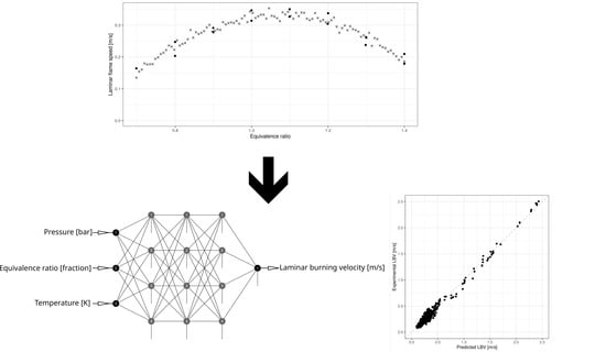
4. Model Construction, Tuning, and Training

The two models were built with the following assumptions about their architectures:

• Initial conditions: 1 atm, 300 K;
• Three inputs: pressure (bar), temperature (K), and equivalence ratio (fractional form);
• One output: LBV (m/s);
• Hidden layers activation functions: hyperbolic tangent;
• Output layer activation function: identity.

The exact model structure, including the number of hidden layers, the number of nodes in each layer, and the L2 regularization parameter [49], was derived by means of a hyperparameter grid search [50] using the following constraints:

• The number of hidden layers ranging from 1 to 4;
• The number of nodes (equal in every hidden layer) between 2 and 5;
• The regularization parameter: ${10}^{-3}$, ${10}^{-4}$, ${10}^{-5}$, ${10}^{-6}$, ${10}^{-7}$, or 0.

In order to develop the models, we used R programming language and FCNN4R package [51]. Using a 5-fold cross-validation [52], all combinations of described hyperparameters were evaluated on the training set. Cross-validation is a method of subsequently dividing (folding) the data into two parts, then training the algorithm on one of the parts and evaluating its performance on the other. The overall performance is usually a mean value calculated from all the folds. This technique helps to prevent overfitting, which can be noticed when algorithms produce good results on the data they were trained on (or very similar data), but they do not generalize and perform poorly on the data not included in training [44]. We used Rprop [53] algorithm to optimize the ANN weights. It was set to minimize the mean squared error (MSE) between the training dataset and predictions. Data scaling to the range of [−1,1] was applied before model tuning and training, with the aim to reduce the training time and help the algorithm to converge. The result of the model tuning phase was the following optimal hyperparameters: 3 hidden layers with 4 nodes each and the L2 regularization coefficient equal to ${10}^{-7}$. Based on the fact that the optimal architecture of both models resulted in the same setup, it can be assumed that in case of applying such modeling for different mixtures, a good choice of the architecture would be the one considered in this work. The final model visualization is presented in Figure 3.

5. Model Validation

Subsequently to model tuning and training, each model’s predictions were compared to the raw experimental data for the corresponding mixture.

Table 1. Models and reference analytical formulas performance metrics on the test (experiments) dataset. ANN—artificial neural network.

	Mean Absolute Error (m/s)	Mean Absolute Percentage Error (%)	R-Squared
ANN H2—air	0.3023	15.69	0.9192
Analytical formula H2—air	1.5118	34.78	0.7014
ANN C3H8—air	0.047	15.89	0.9755
Analytical formula C3H8—air	0.0641	14.71	0.9089

shows the metrics which outline the performance of the models. R-squared (R²) is an indicator that shows the variability and quality of the fit between model and data. The closer to 1, the better [54]. In addition to the models’ performance, analytical formulas were tested for reference metrics. Used formulas were chosen based on the ones that can be found in ddtFoam [55], an open-source Deflagration-to-Detonation solver for OpenFoam software [56], as the aim is to implement the developed LBV models in a modified solver. For hydrogen–air mixture, we used Ardey’s [57] formula (3) as a reference:

$$\begin{array}{cc}\hfill s_{L0}& =-40452·y_{H_2}^4+21026·y_{H_2}^3-3721.6·y_{H_2}^2+238.11·y_{H_2}-1.5938\hfill \\ \hfill s_L& =s_{L0}{\left(\frac{T}{T_{ref}}\right)}^{\alpha }{\left(\frac{p}{p_{ref}}\right)}^{\beta },\hfill \end{array}$$

(3)

where

$s_{L0}$	—LBV of hydrogen–air mixture in reference conditions;
$y_{H_2}$	—mass fraction of hydrogen in the mixture;
$s_L$	—LBV of hydrogen–air mixture in given conditions;
$T_{ref}$	—reference temperature, 298 K;
$p_{ref}$	—reference pressure, $1.013·{10}^5$ Pa;
p	—pressure the LBV is calculated for (Pa);
T	—temperature the LBV is calculated for (K);
$\alpha$	—mixture-specific constant, $1.75$;
$\beta$	—mixture-specific constant, $-0.2$;

while for propane–air, we used Gülder’s [20] formula (4):

$$\begin{array}{cc}\hfill s_{L0}& =0.396{\varphi }^{0.12}exp(-4.95{(\varphi -1.075)}^2)\hfill \\ \hfill s_L& =s_{L0}{\left(\frac{T}{T_{ref}}\right)}^{\alpha }{\left(\frac{p}{p_{ref}}\right)}^{\beta },\hfill \end{array}$$

(4)

where

$s_{L0}$	—LBV of hydrogen–air mixture in reference conditions;
$\varphi$	—equivalence ratio of propane–air mixture;
$s_L$	—LBV of hydrogen–air mixture in given conditions;
$T_{ref}$	—reference temperature, 298 K;
$p_{ref}$	—reference pressure, $1.013·{10}^5$ Pa;
p	—pressure the LBV is calculated for (Pa);
T	—temperature the LBV is calculated for (K);
$\alpha$	—mixture-specific constant, $1.624$;
$\beta$	—mixture-specific constant, $-0.301$.

Table 1 shows that ANN model performed well and was clearly better at calculating LBV than the exemplary analytical models. R-squared for both mixtures was above 0.9 (0.9192 and 0.9755 for hydrogen–air and propane–air, respectively), which indicates adequate fix and capturing of the variability in the data. When investigating mean absolute percentage error (MAPE), one can notice that for both models they are very similar (15.69 and 15.89). This, along with the high R-squared values, indicates that models work equally well for both mixtures and are not dependent on the fuel. MAPE of the order of 15% looks like a good place to improve the models, but one needs to notice the mentioned high-variability and high-spread of experimental data. Based on that, such errors are expected. Looking into the performance of the analytical models, it may be noticed that MAPE of the propane–air formula is actually lower than that of the ANN model. Additionally, other metrics like R-squared and mean absolute error look very good for this formula. However, it needs to be noted that a lower MAPE for the formula resulted in a lower (worse) R-squared. This indicates that there is always a trade-off in how models fit the data, and that above a certain threshold, it is hard to continue improving without sacrificing other properties. The ANNs performed well in optimizing the fit and making it adequate in every case. The supremacy of ANN models may be clearly seen in Figure 4, Figure 5, Figure 6 and Figure 7, which show comparisons of experimental vs. calculated values for hydrogen–air analytical formula and ANN, and propane–air formula and ANN, respectively. The closer the points to the diagonal (the dotted line), the better the fit. Especially in Figure 6, it can be observed that the fit for the formula for propane–air is acceptable for small velocities; however, for the larger ones (above approximately 1 m/s), the formula highly underestimates the LBV values. Such spread and inconsistency are not observable in Figure 7, which represents the fit of the ANN model for propane–air. Here, errors are evenly distributed across the values of the LBV. For hydrogen, Figure 4 shows high error and inadequate fit of the formula, which confirms numbers found in Table 1. The formula highly overestimates the LBV for this mixture, while Figure 5 clearly shows a much better fit. Obviously, some spread can also be seen, but as mentioned before, this spread is to be associated with the high variability, uncertainty, and the nature of the experimental measurements of LBV.

Figure 8, Figure 9 and Figure 10 show exemplary plots of experimental data, analytical formulas, and ANN predictions over variable pressure, equivalence ratio, and temperature, respectively, for hydrogen–air mixture. While one variable was assumed changing, the other two variables were left constant. Plots show that ANN is capable of making predictions over all of its inputs and does not indicate any visible loss of accuracy during this task. Values predicted by the ANN stick reasonably closely to the experimental values. The output is very similar for Figure 11, Figure 12 and Figure 13, which present analogous plots but for propane–air mixture. Importantly, as shown by Table 1 and previous paragraphs, the analytical formula performs noticeably better in comparison with the experimental data than its counterpart for hydrogen–air mixture.

6. Conclusions

In this work, multiple deep neural network models for predicting LBV values for hydrogen–air and propane–air mixtures were developed and validated. Additionally, the data preparation process was described in detail as authors believe it was crucial in achieving good performance of the models considered in this work. This process can be further enhanced or even adapted for the use in other modeling tasks that heavily depend on the experimental data. The models’ inputs were pressure (bar), equivalence ratio, and temperature (K). Based on the provided values, models were able to calculate LBV (m/s) values with high accuracy for a wide range of input values. Main metrics: R-squared and MAPE showed an adequate fit and small error, taking into consideration the issues connected with experimental values of LBV mentioned in the “Introduction and Motivation” section. Moreover, the results of the models were compared with exemplary analytical formulas for calculating LBV that are widely used in CFD codes. The developed model outperformed the analytical formulas in how well they fit the data. The analytical formula for propane–air LBV values also resulted in a good performance, achieving smaller MAPE than the ANN model. However, as could be noticed in the plots later on, it sacrificed the fit to the data, especially for the larger LBV values, which proved that ANNs can asses those kinds of situations and adapt accordingly, resulting in the most optimal fit. The successful development of both models demonstrated that ANNs can be used to model LBV of many mixtures, not only those considered in this work. It was shown that the cited publications also prove this statement. It occurred that the only requirement for developing such models is the availability of the data. Summing up, the ANNs predictions phase is fast enough to be integrated into CFD code and used instead of the analytical formulas to achieve higher accuracy of LBV-based models without sacrificing a noticeable amount of the simulation time.

Models developed in this work can be accessed via the link provided in the supplementary materials.

References

1. von Karman, T.; Penner, S. Fundamental approach to laminar flame propagation. In Selected Combustion Problems; Butterworths Scientific: London, UK, 1954. [Google Scholar]
2. Gibbs, G.J.; Calcote, H.F. Effect of Molecular Structure on Burning Velocity. J. Chem. Eng. Data 1959, 4, 226–237. [Google Scholar] [CrossRef]
3. Rallis, C.J.; Garforth, A.M. The determination of laminar burning velocity. Prog. Energy Combust. Sci. 1980, 6, 303–329. [Google Scholar] [CrossRef]
4. Farrell, J.T.; Johnston, R.J.; Androulakis, I.P. Molecular Structure Effects on Laminar Burning Velocities at Elevated Temperature and Pressure; SAE Technical Paper Series; SAE International: Warrendale, PA, USA, 2004. [Google Scholar] [CrossRef]
5. Ballal, D.; Lefebvre, A. The structure and propagation of turbulent flames. Proc. R. Soc. Lond. A Math. Phys. Sci. 1975, 344, 217–234. [Google Scholar]
6. Wacks, D.H.; Chakraborty, N. Flame Structure and Propagation in Turbulent Flame-Droplet Interaction: A Direct Numerical Simulation Analysis. Flow Turbul. Combust. 2016, 96, 1053–1081. [Google Scholar] [CrossRef] [Green Version]
7. Ravi, S.; Sikes, T.; Morones, A.; Keesee, C.; Petersen, E. Comparative study on the laminar flame speed enhancement of methane with ethane and ethylene addition. Proc. Combust. Inst. 2015, 35, 679–686. [Google Scholar] [CrossRef]
8. Poinsot, T.; Veynante, D. Theoretical and Numerical Combustion; R.T. Edwards, Inc.: Flourtown, PA, USA, 2005; Volume 28. [Google Scholar]
9. White, B.W.; Rosenblatt, F. Principles of Neurodynamics: Perceptrons and the Theory of Brain Mechanisms. Am. J. Psychol. 1963, 76, 705. [Google Scholar] [CrossRef] [Green Version]
10. Rumelhart, D.E.; Hinton, G.E.; Williams, R.J. Learning representations by back-propagating errors. Nature 1986, 323, 533–536. [Google Scholar] [CrossRef]
11. Lecun, Y.; Bottou, L.; Bengio, Y.; Haffner, P. Gradient-based learning applied to document recognition. Proc. IEEE 1998, 86, 2278–2324. [Google Scholar] [CrossRef] [Green Version]
12. Tompson, J.; Schlachter, K.; Sprechmann, P.; Perlin, K. Accelerating Eulerian Fluid Simulation with Convolutional Networks. arXiv 2016, arXiv:1607.03597. [Google Scholar]
13. Shang, Z. Application of artificial intelligence CFD based on neural network in vapor–water two-phase flow. Eng. Appl. Artif. Intell. 2005, 18, 663–671. [Google Scholar] [CrossRef]
14. Elkamel, A.; Al-Ajmi, A.; Fahim, M. Modeling the hydrocracking process using artificial neural networks. Pet. Sci. Technol. 1999, 17, 931–954. [Google Scholar] [CrossRef]
15. Ibargüengoytia, P.H.; Delgadillo, M.A.; García, U.A.; Reyes, A. Viscosity virtual sensor to control combustion in fossil fuel power plants. Eng. Appl. Artif. Intell. 2013, 26, 2153–2163. [Google Scholar] [CrossRef]
16. Pearl, J. Bayesian networks: A model of self-activated memory for evidential reasoning. In Proceedings of the 7th Conference of the Cognitive Science Society, University of California, Irvine, CA, USA, 15–17 August 1985; pp. 15–17. [Google Scholar]
17. Duer, S. Assessment of the Operation Process of Wind Power Plant’s Equipment with the Use of an Artificial Neural Network. Energies 2020, 13, 2437. [Google Scholar] [CrossRef]
18. Amirante, R.; Distaso, E.; Tamburrano, P.; Reitz, R. Analytical Correlations for Modeling the Laminar Flame Speed of Natural Gas Surrogate Mixtures. Energy Procedia 2017, 126, 850–857. [Google Scholar] [CrossRef]
19. Wallesten, J.; Lipatnikov, A.; Chomiak, J. Modeling of stratified combustion in a direct-ignition, spark-ignition engine accounting for complex chemistry. Proc. Combust. Inst. 2002, 29, 703–709. [Google Scholar] [CrossRef]
20. Gülder, Ö.L. Correlations of Laminar Combustion Data for Alternative S.I. Engine Fuels; SAE Technical Paper Series; SAE International: Warrendale, PA, USA, 1984. [Google Scholar] [CrossRef]
21. Burning Velocities of Ethanol-Air and Ethanol-Water-Air Mixtures. In Dynamics of Flames and Reactive Systems; American Institute of Aeronautics and Astronautics: Reston, VA, USA, 1985; pp. 181–197. [CrossRef]
22. Liao, S.; Jiang, D.; Cheng, Q. Determination of laminar burning velocities for natural gas. Fuel 2004, 83, 1247–1250. [Google Scholar] [CrossRef]
23. Müller, U.; Bollig, M.; Peters, N. Approximations for burning velocities and markstein numbers for lean hydrocarbon and methanol flames. Combust. Flame 1997, 108, 349–356. [Google Scholar] [CrossRef]
24. Hu, E.; Li, X.; Meng, X.; Chen, Y.; Cheng, Y.; Xie, Y.; Huang, Z. Laminar flame speeds and ignition delay times of methane–air mixtures at elevated temperatures and pressures. Fuel 2015, 158, 1–10. [Google Scholar] [CrossRef]
25. Dirrenberger, P.; Gall, H.L.; Bounaceur, R.; Herbinet, O.; Glaude, P.A.; Konnov, A.; Battin-Leclerc, F. Measurements of Laminar Flame Velocity for Components of Natural Gas. Energy Fuels 2011, 25, 3875–3884. [Google Scholar] [CrossRef] [Green Version]
26. Coppens, F.; Deruyck, J.; Konnov, A. The effects of composition on burning velocity and nitric oxide formation in laminar premixed flames of CH4 + H2 + O2 + N2. Combust. Flame 2007, 149, 409–417. [Google Scholar] [CrossRef]
27. Jach, A.; Zbikowski, M.; Malik, K.; Żbikowski, M.; Adamski, K.; Cieślak, I.; Teodorczyk, A. Methane-air laminar burning velocity predictions with machine learning algorithms. In Proceedings of the 23rd International Symposium On Combustion Processes, Rynia, Poland, 3–6 September 2017. [Google Scholar] [CrossRef]
28. Jach, A.; Żbikowski, M.; Teodorczyk, A. Laminar Burning Velocity Predictions of Single-Fuel Mixtures of C1-C7 Normal Hydrocarbon and Air. J. KONES 2018, 25, 227–235. [Google Scholar]
29. Mehra, R.; Duan, H.; Ma, F. Laminar burning velocity of hydrogen and carbon-monoxide enriched natural gas (HyCONG): An experimental and artificial neural network study. Fuel 2019, 246, 476–490. [Google Scholar] [CrossRef]
30. Walter, G.; Wang, H.; Kanz, A.; Kolbasseff, A.; Xu, X.; Haidn, O.; Slavinskaya, N. Experimental error assessment of laminar flame speed measurements for digital chemical kinetics databases. Fuel 2020, 266, 117012. [Google Scholar] [CrossRef]
31. Hornik, K. Approximation capabilities of multilayer feedforward networks. Neural Netw. 1991, 4, 251–257. [Google Scholar] [CrossRef]
32. Csáji, B.C. Approximation with artificial neural networks. Fac. Sci. Etvs Lornd Univ. Hung. 2001, 24, 7. [Google Scholar]
33. Dahoe, A. Laminar burning velocities of hydrogen–air mixtures from closed vessel gas explosions. J. Loss Prev. Process Ind. 2005, 18, 152–166. [Google Scholar] [CrossRef]
34. Tse, S.; Zhu, D.; Law, C. Morphology and burning rates of expanding spherical flames in H2/O2/inert mixtures up to 60 atmospheres. Proc. Combust. Inst. 2000, 28, 1793–1800. [Google Scholar] [CrossRef] [Green Version]
35. Dowdy, D.R.; Smith, D.B.; Taylor, S.C.; Williams, A. The use of expanding spherical flames to determine burning velocities and stretch effects in hydrogen/air mixtures. Symp. (Int.) Combust. 1991, 23, 325–332. [Google Scholar] [CrossRef]
36. Egolfopoulos, F.; Law, C. An experimental and computational study of the burning rates of ultra-lean to moderately-rich H2/O2/N2 laminar flames with pressure variations. Symp. (Int.) Combust. 1991, 23, 333–340. [Google Scholar] [CrossRef]
37. Aung, K.; Hassan, M.; Faeth, G. Flame stretch interactions of laminar premixed hydrogen/air flames at normal temperature and pressure. Combust. Flame 1997, 109, 1–24. [Google Scholar] [CrossRef]
38. Kwon, O.; Faeth, G. Flame/stretch interactions of premixed hydrogen-fueled flames: Measurements and predictions. Combust. Flame 2001, 124, 590–610. [Google Scholar] [CrossRef]
39. Kuznetsov, M.; Czerniak, M.; Jordan, T.; Grune, J. Effect of temperature on laminar flame velocity for hydrogen-air mixtures at reduced pressures. In Proceedings of the International Conference on Hydrogen Safety (ICHS 2013), Brussels, Belgium, 9–11 September 2013; p. 231. [Google Scholar]
40. Pareja, J.; Burbano, H.J.; Ogami, Y. Measurements of the laminar burning velocity of hydrogen–air premixed flames. Int. J. Hydrog. Energy 2010, 35, 1812–1818. [Google Scholar] [CrossRef]
41. Ebaid, M.S.; Al-Khishali, K.J. Measurements of the laminar burning velocity for propane: Air mixtures. Adv. Mech. Eng. 2016, 8, 168781401664882. [Google Scholar] [CrossRef]
42. Vagelopoulos, C.; Egolfopoulos, F.; Law, C. Further considerations on the determination of laminar flame speeds with the counterflow twin-flame technique. Symp. (Int.) Combust. 1994, 25, 1341–1347. [Google Scholar] [CrossRef]
43. Vagelopoulos, C.M.; Egolfopoulos, F.N. Direct experimental determination of laminar flame speeds. Symp. (Int.) Combust. 1998, 27, 513–519. [Google Scholar] [CrossRef]
44. Goodfellow, I.; Bengio, Y.; Courville, A. Deep Learning; MIT Press: Cambridge, MA, USA, 2016; Available online: http://www.deeplearningbook.org (accessed on 18 April 2020).
45. Husson, F.; Josse, J.; Narasimhan, B.; Robin, G. Imputation of mixed data with multilevel singular value decomposition. J. Comput. Graph. Stat. 2019, 28, 552–566. [Google Scholar] [CrossRef] [Green Version]
46. Beretta, L.; Santaniello, A. Nearest neighbor imputation algorithms: A critical evaluation. BMC Med. Informatics Decis. Mak. 2016, 16. [Google Scholar] [CrossRef] [PubMed] [Green Version]
47. Qiu, Y.L.; Zheng, H.; Gevaert, O. A deep learning framework for imputing missing values in genomic data. bioRxiv 2018. [Google Scholar] [CrossRef]
48. Triola, M.F. Elementary Statistics, 13th ed.; Pearson: Boston, MA, USA, 2017. [Google Scholar]
49. Hoerl, A.E.; Kennard, R.W. Ridge Regression: Biased Estimation for Nonorthogonal Problems. Technometrics 1970, 12, 55–67. [Google Scholar] [CrossRef]
50. Bergstra, J.S.; Bardenet, R.; Bengio, Y.; Kégl, B. Algorithms for Hyper-Parameter Optimization. In Advances in Neural Information Processing Systems 24 (NIPS 2011); Shawe-Taylor, J., Zemel, R.S., Bartlett, P.L., Pereira, F., Weinberger, K.Q., Eds.; Neural Information Processing Systems Foundation: Granada, Spain, 2011; Volume 24. [Google Scholar]
51. Klima, G. FCNN4R: Fast Compressed Neural Networks for R, R Package Version 0.6.2; 2016. Available online: https://www.rdocumentation.org/packages/FCNN4R/versions/0.6.2 (accessed on 18 April 2020).
52. Browne, M.W. Cross-Validation Methods. J. Math. Psychol. 2000, 44, 108–132. [Google Scholar] [CrossRef] [Green Version]
53. Riedmiller, M. Rprop—Description and Implementation Details: Technical Report; Inst. f. Logik, Komplexität u. Deduktionssysteme: Karlsruhe, Germany, 1994. [Google Scholar]
54. Miles, J. R Squared, Adjusted R Squared. In Wiley StatsRef: Statistics Reference Online; American Cancer Society: Hoboken, NJ, USA, 2014. [Google Scholar] [CrossRef]
55. Ettner, F.; Vollmer, K.G.; Sattelmayer, T. Numerical Simulation of the Deflagration-to-Detonation Transition in Inhomogeneous Mixtures. J. Combust. 2014, 2014, 1–15. [Google Scholar] [CrossRef] [Green Version]
56. Weller, H.G.; Tabor, G.; Jasak, H.; Fureby, C. A tensorial approach to computational continuum mechanics using object-oriented techniques. Comput. Phys. 1998, 12, 620–631. [Google Scholar] [CrossRef]
57. Ardey, N. Struktur und Beschleunigung Turbulenter Wasserstoff-Luft-Flammen in Räumen mit Hindernissen; NA: München, Germany, 1998. [Google Scholar]
Figure 1. Simulated mean laminar burning velocity (LBV) (line) for H2–air, as a function of equivalence ratio. Dots represent the experimental data.
Energies 13 03381 g001
Figure 2. Simulated points (crosses) for C3H8–air, as a function of equivalence ratio. Dots represent the experimental data.
Energies 13 03381 g002
Figure 3. Final model schema
Energies 13 03381 g003
Figure 4. Formula calculations vs. experiments comparison for H2–air mixture.
Energies 13 03381 g004
Figure 5. Model prediction vs. experiments comparison for H2–air mixture.
Energies 13 03381 g005
Figure 6. Formula calculations vs. experiments comparison for C3H8–air mixture.
Energies 13 03381 g006
Figure 7. Model prediction vs. experiments comparison for C3H8–air mixture.
Energies 13 03381 g007
Figure 8. Exemplary comparison of models predictions, analytical formula calculations, and experiments for variable pressure, constant temperature of 373 K, and constant equivalence ratio of 0.51. H2–air mixture.
Energies 13 03381 g008
Figure 9. Exemplary comparison of models predictions, analytical formula calculations, and experiments for variable equivalence ratio, constant temperature of 373 K, and constant pressure of 1 bar. H2–air mixture.
Energies 13 03381 g009
Figure 10. Exemplary comparison of models predictions, analytical formula calculations, and experiments for variable temperature, constant pressure of 1 bar, and constant equivalence ratio of 0.84. H2–air mixture.
Energies 13 03381 g010
Figure 11. Exemplary comparison of models predictions, analytical formula calculations, and experiments for variable pressure, constant temperature of 350 K, and constant equivalence ratio of 1.1. C3H8–air mixture.
Energies 13 03381 g011
Figure 12. Exemplary comparison of models predictions, analytical formula calculations and experiments for variable equivalence ratio, constant temperature of 644 K, and constant pressure of 1 bar. C3H8–air mixture.
Energies 13 03381 g012
Figure 13. Exemplary comparison of models predictions, analytical formula calculations, and experiments for variable temperature, constant pressure of 1 bar, and constant equivalence ratio of 1. C3H8–air mixture.
Energies 13 03381 g013