Development of Test-Bed Controller for Powertrain of HEV

State Key Laboratory of Automotive Safety and Energy, Tsinghua University, Beijing 100084, China
*
Author to whom correspondence should be addressed.
Energies 2020, 13(13), 3372; https://doi.org/10.3390/en13133372
Submission received: 17 May 2020
/
Revised: 20 June 2020
/
Accepted: 29 June 2020
/
Published: 1 July 2020
(This article belongs to the Section A1: Smart Grids and Microgrids)
Abstract
:The dynamic test-bed is a powerful tool for the powertrain integration and control strategy development of a hybrid electric vehicle (HEV). This paper focuses on developing a test-bed controller with driver simulation, road load simulation (RLS), and engine simulation. The main factors that influence the RLS accuracy are analyzed, especially inertia of test-bed and torque signal sampling frequency, and the RLS algorithm with penalty function based on a forward model is proposed. The engine model is developed and permanent magnet synchronous motor (PMSM) is adopted to realize engine start-up/stop, torque control, and inertia simulation. The simulation platform was built in MATLAB/Simulink to verify its accuracy. The simulation results present the developed RLS with a penalty function based on a forward model that can reduce the speed and torque error. The developed controller is applied to the single-axis parallel HEV test-bed. The experiment results show that the developed test-bed controller can precisely emulate the road load and improve the efficiency of the development of HEV powertrain.
1. Introduction
In recent years, hybrid electric vehicles (HEVs) have been recognized as promising technologies to replace the conventional internal-combustion engine (ICE)-drive road vehicles, improving fuel economy, and reducing harmful tailpipe emissions [1,2,3,4]. The HEV has become a worldwide research hotspot.
In general, HEV adopts the model-based development process, including the off-line simulation, the rapid prototyping, the hardware-in-the-loop simulation, the bench test, and the real vehicle calibration. The role of the test-bed played in the process includes: (1) measuring the performance parameters of components and verifying the reliability of the powertrain of HEV; (2) providing a platform to verify the developed hybrid control strategy; (3) accurate assessment of vehicle dynamics, economy, and emissions performance. In conclusion, the test-bed can comprehensively evaluate the performances of components, powertrain, and energy management strategies of HEV, which has become an essential means to reduce the development cost and improve development efficiency.
The test-bed controller is the core of test-bed, and its function includes constant speed control, constant torque control, and road load simulation (RLS) which is the core of the controller software [5]. RLS is to emulate the road resistance through the dynamometer [6,7]. Hewson adopts the inverse model method to realize the simulation of linear and nonlinear loads [8]. Arellano-Padilla J calculates ideal position response based on the forward model and the real torque generated by the powertrain and controls the dynamometer through position tracker to track the ideal position to realize the load simulation [9,10]. Rodic M analyzed the frequencies characteristics of the tracking method based on the forward model and points out that this algorithm has a certain range of available frequencies in application [11]. The structure of engine is complex, which needs to consider noise and vibration treatment [12,13]. In order to reduce the maintenance cost and improve efficiency, the engine simulation algorithm in this paper is developed to realize the engine function through a permanent magnet synchronous motor (PMSM) which is called an engine motor.
This paper is organized as follows. Section 2 represents the structure and components of the test-bed. Section 3 researches the control strategy of the test-bed controller driver model, the RLS based on a forward model based on the penalty function and engine simulation. Section 4 presents the model of test-bed and the tested powertrain of HEV to verify the developed RLS. Section 5 builds the test-bed for the single parallel hybrid powertrain system to verify the accuracy of developed RLS and engine simulation. Section 6 concludes the main points of this research.
2. Structure of Test-Bed
The test-bed consists of two parts, namely the hardware part and the control system. The hardware part contains tested powertrain of HEV, torque meter, data acquisition system, dynamometer system, and other devices. The control system includes a real-time test-bed controller and a host computer. The structure of a single dynamometer test-bed including engine simulation is shown in Figure 1.
The test-bed controller adopts the embedded industrial computer with the real-time operating system (RTOS), which controls the dynamometer to achieve different control modes, including speed control mode, torque control mode, and RLS mode which is the core of the controller. In the RLS mode, the driver model calculates the accelerator pedal opening and brake pedal opening which are transmitted to the hybrid control unit (HCU). HCU will calculate the demand torque and send the control commands to the vehicle components, such as engine, motor, clutch, and gear. RLS model emulates the road resistance load by the dynamometer. The tested powertrain of HEV and dynamometer working together forms a closed-loop. The control strategy of the controller is developed based on LabVIEW. The structure of the controller is presented in Figure 2.
The test-bed controller includes the hardware and software in Figure 2. The hardware includes the CAN communication board and DAQ (data acquisition) board, and the software includes the model of driver/engine/RLS (road load simulation). The controller collects the signals of the sensors through the hardware. Additionally, the software analyzes and calculates the input information and outputs the command to the dynamometer system through the hardware (CAN board and DAQ board).
3. Test-Bed Control Strategy
3.1. RLS with a Penalty Function Based on a Forward Model
The basic principle of RLS based on the forward model is to use the torque generated by the powertrain of HEV to drive the vehicle model to get the target rotation speed and control the dynamometer to track that speed to simulate the real road resistance [14,15]. The RLS based on the forward model is more stable, because it avoids differential calculations. The process is shown in Figure 3.
In Figure 3, is the torque generated by the powertrain. is the vehicle transfer function. is the target rotation speed. is the actual dynamometer speed. is the speed tracker. is the theoretical resistance torque. is the actual resistance torque generated by the dynamometer. is the torque response function of the dynamometer.
According to Figure 3, Equation (1) can be obtained.
There is a vehicle transfer function at the right side of the Equation (1), which causes great inconvenience to analyze the RLS based on a forward model targeted at a different type of vehicle. Ideally, the right side of the Equation (1) only contains property parameters of the test-bed. Equation (1) should be transformed. As can be considered as 1, the RLS based on the forward model in Figure 3 is transformed to that in Figure 4.
In Figure 4, is equal to and that is considered to be an interference, which has a great effect on the accuracy of the RLS based on the forward model. We can get the transformation of Equation (1) as Equation (2).
In Equation (2), is a speed tracker with the PI regulator, which can be approximated by Equation (3) where is the scale factor and is the integral factor. is the transfer function of the test-bed, which is represented by Equation (4) where and are the sums of moments of inertia and damping of the rotation parts of the test-bed. If the test-bed contains the gearbox, and vary depending on gear.
At steady state, the value is constant and is equal to 1, which indicts that the actual speed is equal to the target speed and the test-bed can accurately emulate the road resistance. At dynamic state, the frequency of is not equal to 0 and is not equal to 1, so there is the gap between the simulated load and the actual load.
The penalty function is added after the vehicle transfer function to eliminate the error. Figure 5 shows the transfer function graph. As Equation (6) presents, there is no deviation between the simulated load and the actual load, which verifies that the algorithm satisfies the full simulated road load without interference.
The transfer function of the penalty function is presented as Equation (7) and the order of the numerator is larger than the denominator which causes the system to be unstable, so the first-order inertia shown in Equation (8) is added to the . The penalty function becomes Equation (9). After adding the penalty function, the transfer function is shown as Equation (10). If the time constant is small enough, the right end of the equation is approximately equal to 1, and the simulated load is infinitely close to the actual load.
Next, we consider how to eliminate or reduce the interference of . The interference effect of is equal to which can be measured by the torque meter and can be compensated by adding interference function as shown in Figure 6.
If is equal to 1, the interference is completely canceled. In fact, due to the delay of the data acquisition itself, cannot be equal to 1. It can be considered that is a first-order inertia link. As shown in Equation (15), the magnitude of the time constant depends on the data acquisition frequency. After the sampling penalty, the interference on the output of the test-bed is as shown in Equation (12).
3.2. Driver Model
The driver model simulates the real driver’s behavior to track velocity by adjusting the accelerator pedal and brake pedal. The emulation algorithm of the driver model is shown in Figure 7.
The driver model is mainly composed of velocity closed-loop control and torque closed-loop control. The PI regulators are commonly used for closed-loop control. Taking the velocity closed-loop control as an example and the expression is shown as follows:
In the formula, is the target velocity; is the actual velocity which is derived from the dynamometer. is the target torque calculated by the test-bed controller based on the target velocity and the actual velocity.
4. Simulation and Results Discussion
The simulation platform including the powertrain model of a pure electric SUV, the dynamometer model, and the controller of test-bed was built in MATLAB/Simulink to test the developed RLS and driver model. Table 1 shows the parameters of the vehicle and the test-bed. The New European Driving Cycle (NEDC) was adopted as the tested cycle. The simulation platform developed based on MATLAB/Simulink is shown in Figure 8.
According to Figure 9, the maximum difference between the cycle velocity and actual velocity does not exceed , which illustrates that the powertrain and parameters of the vehicle are matched, and the driver model can accurately track the target velocity by adjusting the accelerator pedal and brake pedal. Figure 10 shows the difference between the target rotation speed and the actual rotation speed of the dynamometer does not excel 4 r/min, which illustrates that the theoretical analysis and simulation results are consistent.
Figure 11 presents the theoretical resistance torque and the torque of the drive motor which is the only power resource of the vehicle. The theoretical resistance torque is the product of the target rotation speed and the vehicle inverse model , and the expression in the time domain is shown as Equation (14). It is known that the transfer function between the theoretical resistance torque and the dynamometer torque is the first order inertia link with a time constant without considering the interference of The difference between the two does not exceed which verifies the theoretical analysis and simulation results are in agreement.
where is the wheel radius and is the main reducer reduction ratio. , , , , and represent rolling resistance, wind resistance, grade resistance, acceleration resistance, and mechanical braking resistance, respectively.
4.1. Impact of Inertia on RLS
The inertia and damping are presented in all test-bed systems. As the coefficient of inertia is quadratic, it has the greater influence on the test-bed. The impact of that on the RLS was studied by a single variable method. Since the NEDC data is too large, the data of the first were selected for analysis. Figure 12a shows the simulation results of the developed RLS with the penalty function based on a forward model when the inertia is . Figure 12b–d presents the simulation results of the RLS without the penalty function based on the forward model when the inertia of the test-bed is , , and , respectively. According to the comparison among Figure 12b–d, the accuracy of the RLS is lower with the inertia of the test-bed increasing, which is consistent with the previous theoretical analysis.
Table 2 shows the simulation results of the whole NEDC cycle. The simulation results indicate that when the inertia of the test-bed is , the maximum speed and torque error percentage of RLS with the penalty function is reduced from and to and , respectively, compared with that without the compensation function.
4.2. Impact of the Sampling Frequency on RLS
From the previous theoretical analysis, the influence of the interference on the rotation speed of the test-bed is as shown in Equation (15).
Figure 13a,b shows the simulation results when the sampling frequency is and . According to the comparison, the consistency between the target rotation speed and the actual rotation speed of the dynamometer is worse as the sampling frequency drops down. The deviation between the theoretical resistance torque and the motor torque is also larger which causes lower RLS accuracy. The simulation result of the RLS without penalty function based on the forward model is shown in Figure 13c. The deviation between the target rotation speed and the actual rotation speed is too large to meet the test requirements. Table 3 shows the simulation results of the NEDC cycle.
Table 3 shows the simulation results of the RLS with the different sampling frequencies under the NEDC cycle. When the sampling frequency is , the maximum speed and torque error percentage of the RLS with penalty function is reduced from and to and , respectively, compared with the RLS without the penalty function. Additionally, the accuracy of RLS is lower with the sampling frequency decreasing.
4.3. Engine Simulation
The engine motor needs to emulate the operation process of the engine including start, stop, idle, speed control, torque control, speed control, and engine friction losses such as pumping losses, and accessory loss. Engine motor torque consists of three parts, idle speed control torque, friction torque, and the torque command of HCU. HCU outputs many signals to the engine simulation model, including idle speed, idle switch, engine control mode, engine target torque, engine target speed, etc. The engine simulation model outputs target torque to the engine motor to emulate the performance of the engine. The algorithm of engine simulation is shown in Figure 14 and Figure 15.
Idle speed control torque is to emulate the idle state of the engine. If the idle switch is off, the idle torque is 0. If the idle switch is on, the idle torque is as shown in Equation (16). Friction torque is the function of the speed, so it can be looked up through a table.
is the idle speed of the engine motor, is the actual speed of the engine motor, is the idle control torque of the engine motor.
When the engine control mode is the torque mode, if the inertia simulation is not considered, the HCU target torque is the engine motor target torque. If the inertia simulation is needed, the engine inertia simulation module can be used to calculate the target rotation speed, and then the engine motor is to track the rotation speed. The inertia simulation module algorithm is shown in Equation (17) and the speed tracking adopts a PI regulator. When the engine control is the speed mode, the target torque of the engine motor can be calculated by the PI regulator and the input of the regulator is the target speed and the actual of the engine motor.
is the target speed of the engine motor, is the engine simulated torque, is the actual engine torque, and is the inertia of the simulated engine.
5. Test Platform Construction and Experiment
5.1. Test Platform Construction
The test-bed controller is based on the National Instruments (NI) PXI hardware including the PXIe-8100 processor board, PXI-8512 CAN communication board, and PXI-8221 data acquisition board and the real-time operating system (RTOS). The RTOS runs multi-tasking in parallel, such as host computer communication, CAN communication, and control algorithm. The main task of the test-bed controller is to read the information of the external device through the CAN network, including the speed, torque, throttle position, and receive the host computer control commands and front panel commands. Additionally, the controller calculates the command and then sends those commands to the dynamometer.
The test-bed system adopts a ABB ACS800 inverter cabinet and HBM T10F torque meter. Additionally, the range of the torque meter is and the accuracy is up to . The test-bed built for the single-axis parallel hybrid system is shown in Figure 16.
5.2. RLS Experiment
The tested objective is a single-axis parallel hybrid bus and the parameters of the vehicle are shown in Table 4. China City Bus Cycle (CCBC) was adopted as the test cycle and the test results are presented in Figure 17, Figure 18 and Figure 19.
Figure 17a,b shows the velocity tracking curves, the accelerator pedal signal, and the brake pedal opening. According to the figure, the difference between the target velocity and the actual velocity in the range of is no more than , but that in the last part of the cycle is quite different. It is known that the accelerator pedal is at this time, and the powertrain is working at full load. It can be inferred that the powertrain output torque is insufficient at this time, so the actual vehicle speed cannot track the target vehicle speed.
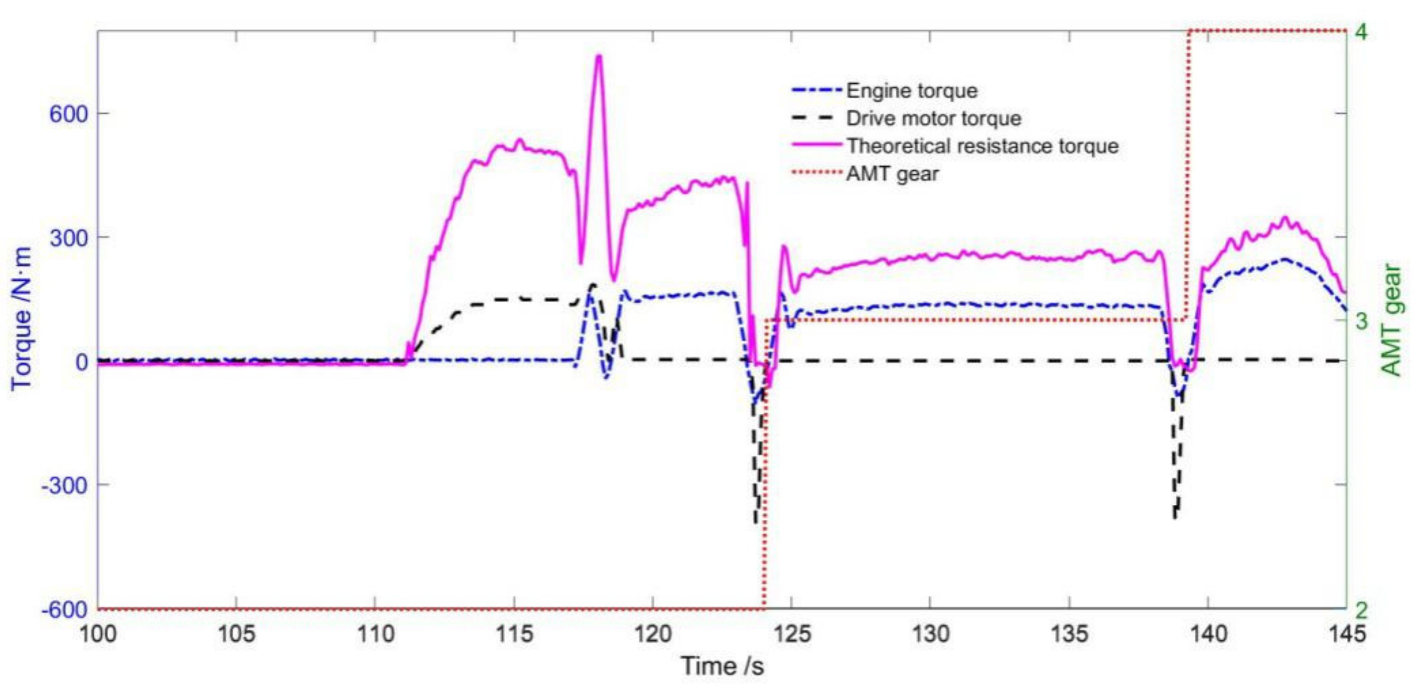
Figure 18 displays the torque curve of each component during the test, and data was selected for analysis. When the vehicle starts, the motor is driving separately; the engine does not output torque; when the engine starts, the motor output torque is , the engine works alone. When the driver brakes, the motor outputs negative torque for braking energy recovery. The vehicle starts at 2nd gear and shifts according to the vehicle speed and the accelerator pedal opening. Since the load system is connected to the output shaft of the transmission, the torque of the load system is approximately equal to the torque produced by the engine and the motor.
Figure 19 is the verification of the developed RLS. Figure 19a displays the target rotation speed and the actual rotation speed. The target rotation speed is calculated by the torque generated by the power system driving the virtual vehicle model. For comparison, the target rotation speed is converted to the transmission output shaft speed. The actual speed is the output shaft speed of the gearbox. As can be seen from the figure, the difference between the target speed and the actual speed is small and almost coincides. Figure 19b is the curve of the theoretical resistance torque and the output torque of the powertrain system. The theoretical resistance torque is the torque that the powertrain system needs to overcome when the vehicle is running on the road. For comparison, the torque is also converted to the output shaft of the transmission. Since the inertia of the test-bed and the angular accelerator of the rotation are small, the output torque of the powertrain system can be approximated by the measured value of the torque meter. It can be seen that the theoretical resistance torque is consistent with the output torque of the powertrain system. Figure 19 verifies that the accuracy of the developed RLS with a penalty function based on the forward model is reliable.
5.3. Engine Simulation Experiment
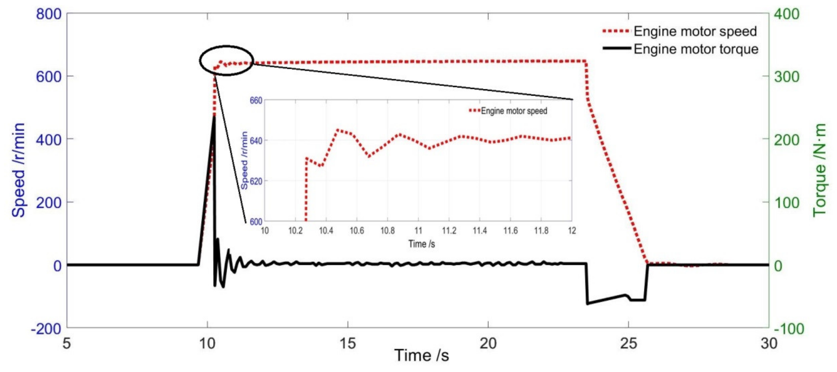
Figure 20 shows the process of engine start-stop control. At , the test-bed controller receives the engine start command from the HCU and sends the start torque command to the engine motor. The engine motor rapidly rises to the idle speed about , completing the start-up process, and the start-up process takes about . After the speed of the engine motor reaches the idle speed, it would fluctuate around the idle speed. During the start process, the fluctuation range of the speed does not exceed 10 r/min, which illustrates that the start process is quite smooth.
During the time of , the engine motor maintains idle state. The test-bed controller controls the engine motor speed to stabilize at , and the upper and lower fluctuations are . As the engine motor’s rotational resistance torque is small, the engine motor’s output torque is also small. At , the controller receives the stop command from the HCU. The engine motor simulates the engine resistance. The engine motor rapidly decreases to under the action of the engine resistance. The stop command is completed, and the shutdown process takes about .
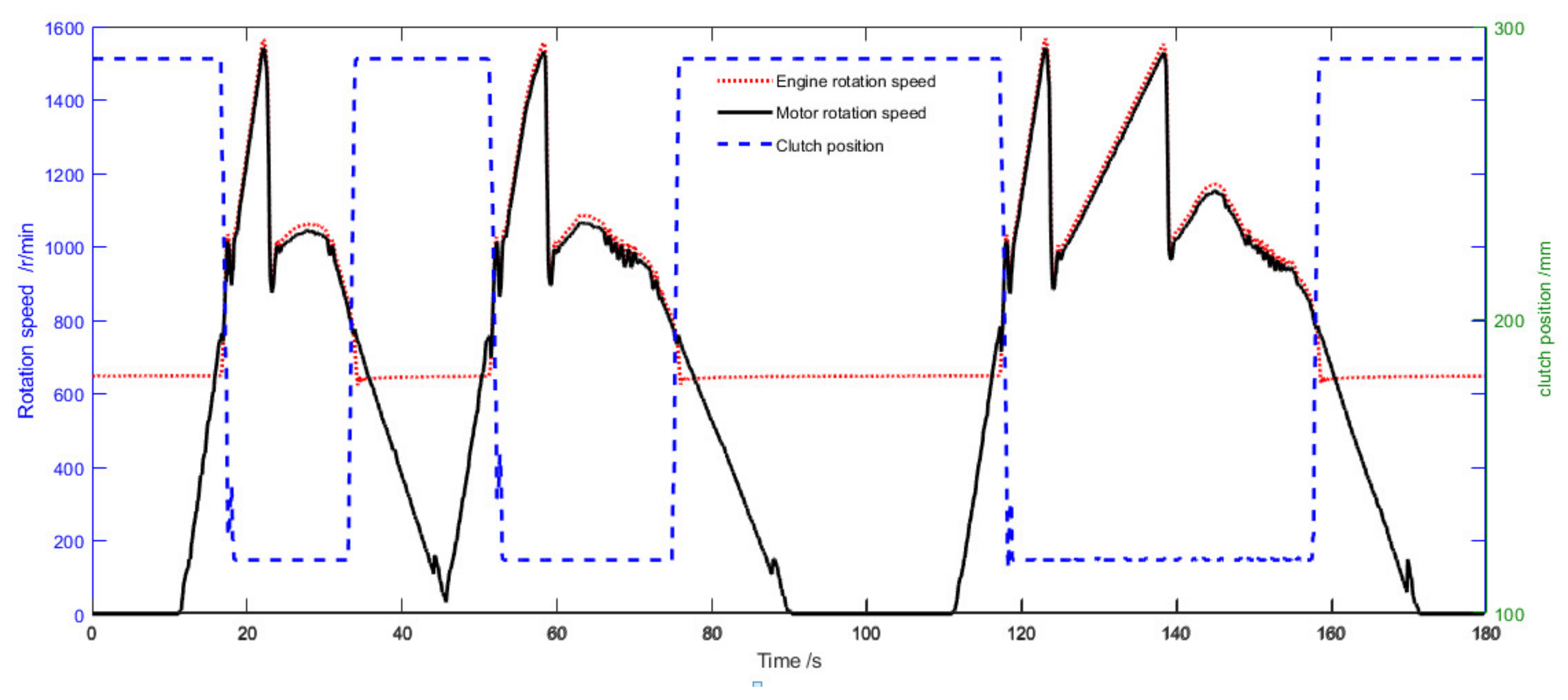
Figure 21 shows the engine motor as the engine participation in the drive process. At the start, the transmission shaft speed is lower than the engine idle speed, the clutch is disengaged, the engine maintains idle speed, and the motor drives the vehicle to accelerate separately. When the transmission shaft speed is higher than the engine idle speed, the clutch is engaged When the clutch is engaged, the speed of engine is equal to the speed of motor. Due to the shift mode without the clutch, the clutch does not need to be separated during the shifting process. When the vehicle is stopped, the velocity of the vehicle is reducing. When the transmission input shaft speed is lower than the engine idle speed, the clutch is separated, and the engine maintains idle speed state and waits for the next clutch engagement.
6. Conclusions
This paper focused on the development of a test-bed controller with the driver simulation, RLS, and engine simulation. Factors that mainly influence the RLS accuracy were analyzed, especially the inertia of test-bed and the sampling frequency of torque. The RLS with the penalty function based on the forward model was proposed. Simulation results show that the developed driver model and RLS are accurate and reliable, meeting the requirements of the bed test. The engine simulation realized simulation of the engine characteristics through motor control and this paper focused on the functions of starting, stopping, idling, rotation speed control, and torque control of the engine. To verify the developed controller in a real environment, the test-bed with engine simulation for a single parallel powertrain of HEV was built. The test results show that the developed controller with driver simulation, RLS with penalty function based on the forward model, and engine simulation can meet the test requirements well.
Author Contributions
P.L. wrote the manuscript, constructed the simulation model and developed the control strategy of the controller. Y.H. was responsible for revising the manuscript and analyzing the data. L.Z. was responsible for revising the formant and translating the paper. Z.J. was responsible for the manuscript supervising. All authors have read and agreed to the published version of the manuscript.
Funding
This research was funded by National Key R&D Plan (Grant No.2016YFB0101402). The authors are also grateful for the sponsorship from the Special fund for collaborative innovation of Foshan-Tsinghua University industry research cooperation (THFS01).
Conflicts of Interest
The authors declare no conflict of interest.
References
- Ouyang, M. Development and Prospect of New Energy Vehicles in China. Sci. Technol. Rev. 2016, 34, 13–20. [Google Scholar]
- Niu, J.G.; Pei, F.L.; Zhou, S.; Zhang, T. Multi-objective Optimization Study of Energy Management Strategy for Extended-Range Electric Vehicle. Adv. Mater. Res. 2013, 694–697, 2704–2709. [Google Scholar] [CrossRef]
- Gong, C.; Hu, M.; Li, S.; Zhan, S.; Qin, D. Equivalent consumption minimization strategy of the hybrid electric vehicle considering the impact of driving style. Proc. Inst Mech. Eng. Part D J. Automob. Eng. 2018, 233, 2610–2623. [Google Scholar] [CrossRef]
- Omer, A.M. Energy and environment: Applications and sustainable development. Br. J. Environ. Clim. Chang. 2011, 1, 118–158. [Google Scholar] [CrossRef] [PubMed]
- Gehringer, M.A.; Defenderfer, E.J. Road Load Simulation Testing for Improved Assessment of Powertrain Noise and Vibration. SAE Int. J. Engines 2011, 4, 1210–1216. [Google Scholar] [CrossRef]
- Newton, R.W.; Betz, R.E.; Penfold, H.B. Emulating dynamic load characteristics using a dynamic dynamometer. In Proceedings of the IEEE International Conference on Power Electronics Drive Systems, Singapore, 21–24 February 1995. [Google Scholar]
- Ye, X.; Jin, Z.H.; Gao, D.W.; Lu, Q.C. Dynamometer Controller Algorithm for Road Load Emulations. J. Tsinghua Univ. (Sci. Technol.) 2013, 53, 1492–1497. [Google Scholar]
- Hewson, C.R.; Sumner, M.; Asher, G.M.; Wheeler, P.W. Dynamic mechanical load emulation test facility to evaluate the performance of AC inverters. Power Eng. J. 2000, 14, 21–28. [Google Scholar] [CrossRef]
- Arellano-Padilla, J.; Asher, G.; Sumner, M. Control of an AC Dynamometer for Dynamic Emulation of Mechanical Loads with Stiff and Flexible Shafts. IEEE Trans. Ind. Electron. 2006, 53, 1250–1260. [Google Scholar] [CrossRef]
- Akpolat, Z.H.; Asher, G.M.; Clare, J.C. Experimental dynamometer emulation of nonlinear mechanical loads. IEEE Trans. Ind. Appl. 2002, 35, 1367–1373. [Google Scholar] [CrossRef]
- Rodic, M.; Jezernik, K.; Trlep, M. Dynamic emulation of mechanical loads: An advanced approach. IEEE Proc.-Electr. Power Appl. 2006, 153, 159–166. [Google Scholar] [CrossRef]
- Wu, Z. Development of bench test systems for new energy vehicles. Master’s Thesis, Tsinghua University, Beijing, China, , 2016; pp. 28–34. [Google Scholar]
- Zhu, F.S.; Chen, X.M.; Ye, R.K.; Bao, J.Q. Urban Low-carbon Transport, Model of Pure Electric Vehicle Development Typical Research Based on Hangzhou Pure Electric Taxi Demonstration Operations. In Proceedings of 2013 International Conference on Future Energy & Materials Research, Madison, WI, USA, 24 September 2013. [Google Scholar]
- Zheng, X. Research on chassis dynamometer test technology based on rolling resistance dynamic loading and motion parameter prediction. Master’s Thesis, Zhejiang University, Zhejiang, China, 2018; pp. 32–36. [Google Scholar]
- Li, Q.; Zhao, X. Electrical simulation of resistance of chassis dynamometer based on rapid prototype. Agric. Equip. Veh. Eng. 2019, 57, 7–10. [Google Scholar]
Figure 1.
The layout of a single dynamometer test-bed for the hybrid electric vehicle (HEV).
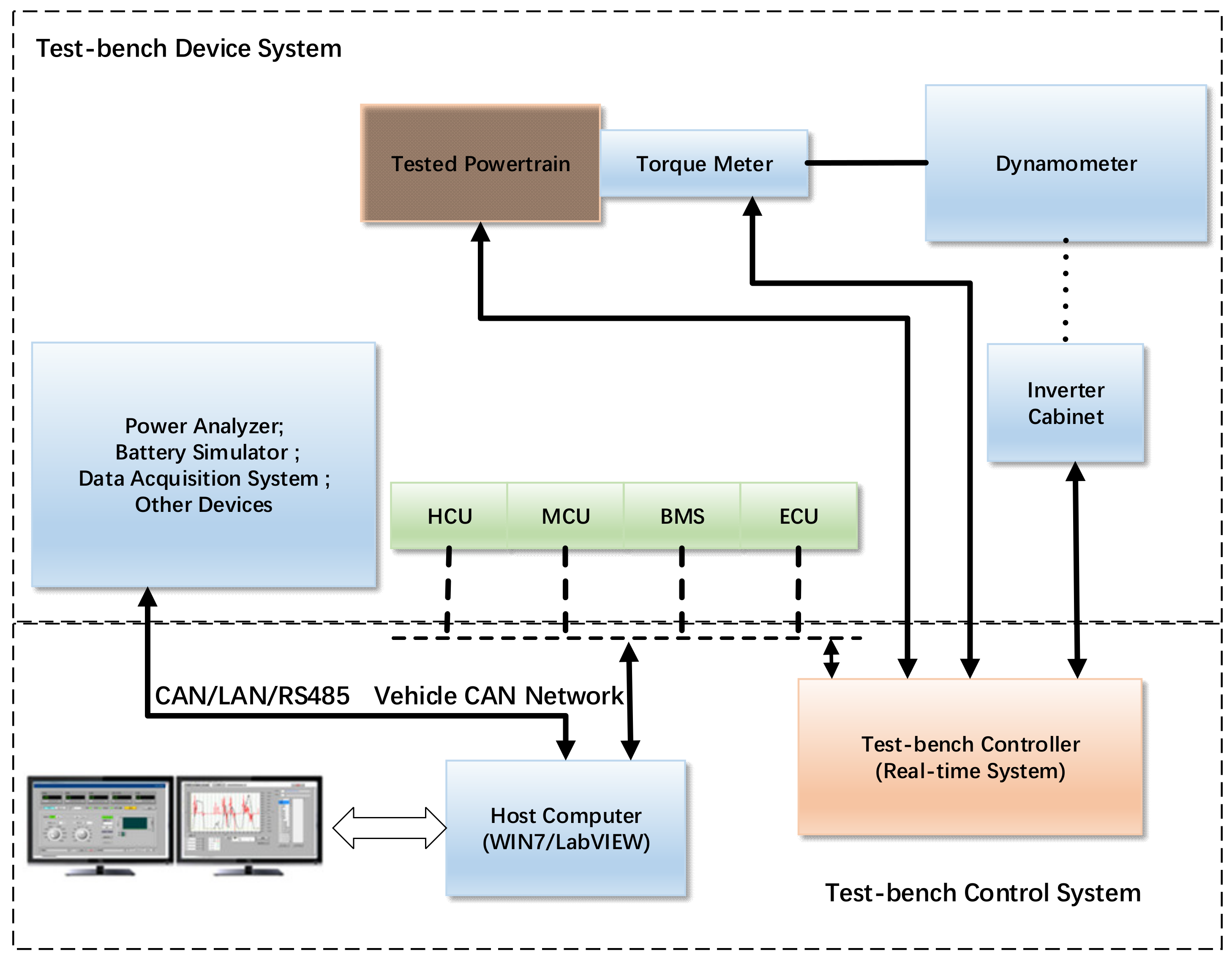
Figure 2.
Structure of test-bed controller.
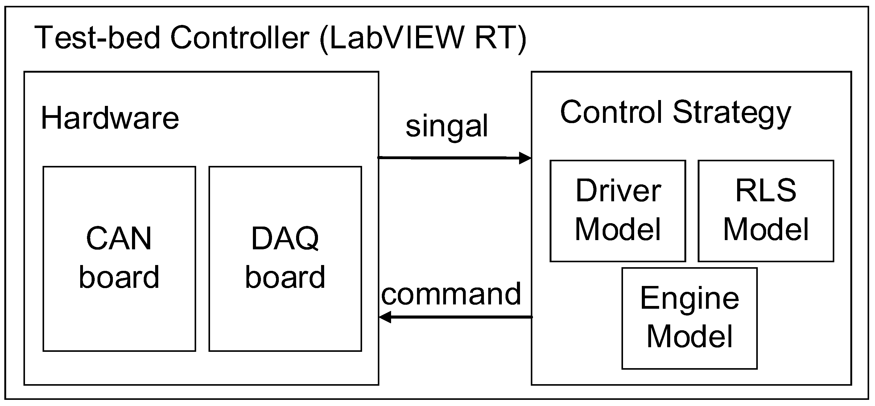
Figure 3.
Process of the road load simulation (RLS) based on the forward model.
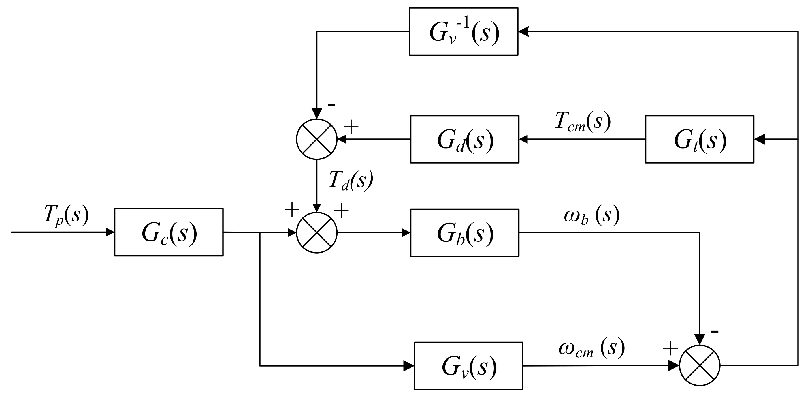
Figure 4.
Simplified RLS based on a forward model.
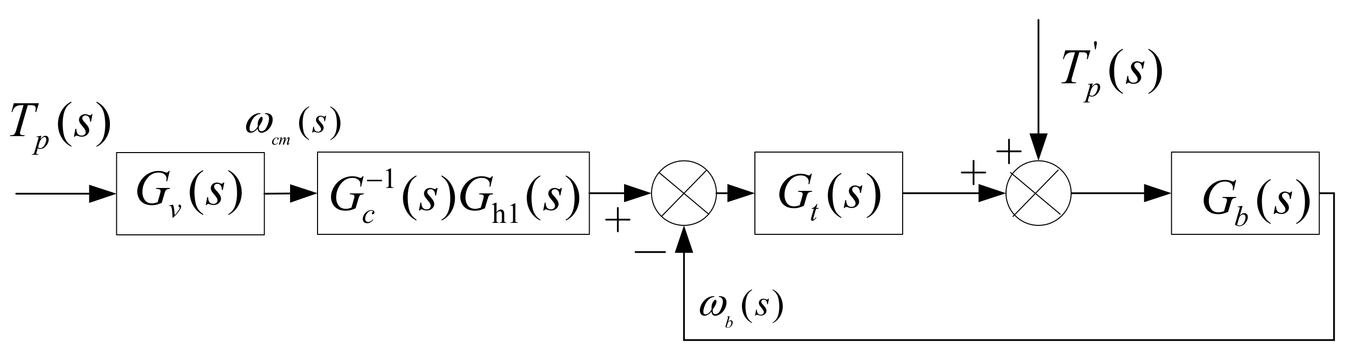
Figure 5.
The transfer function diagram after adding the penalty function.
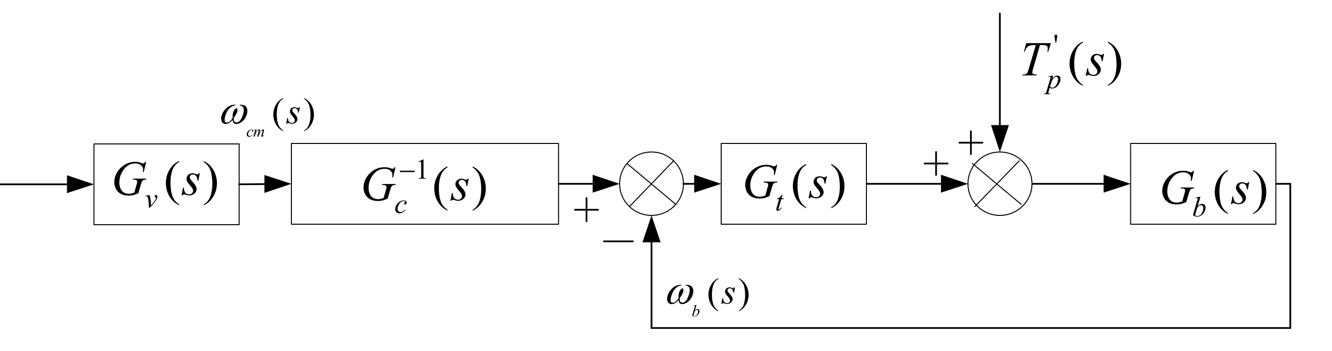
Figure 6.
Transfer function diagram after adding the interference penalty.
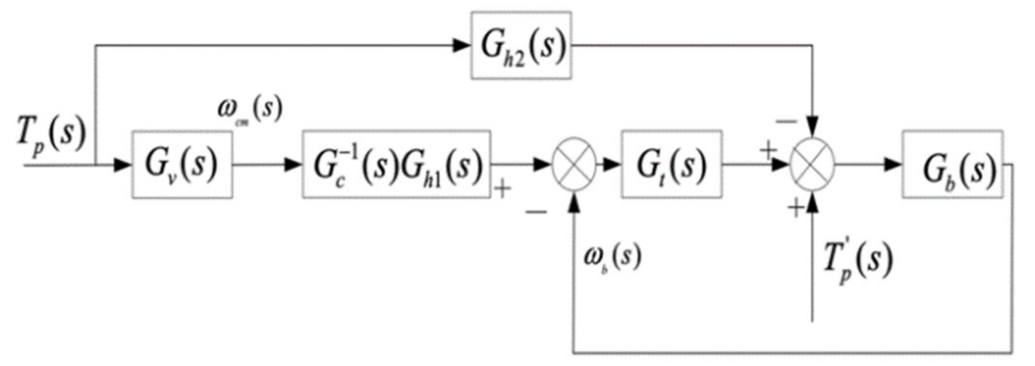
Figure 7.
The emulation algorithm of the driver model.
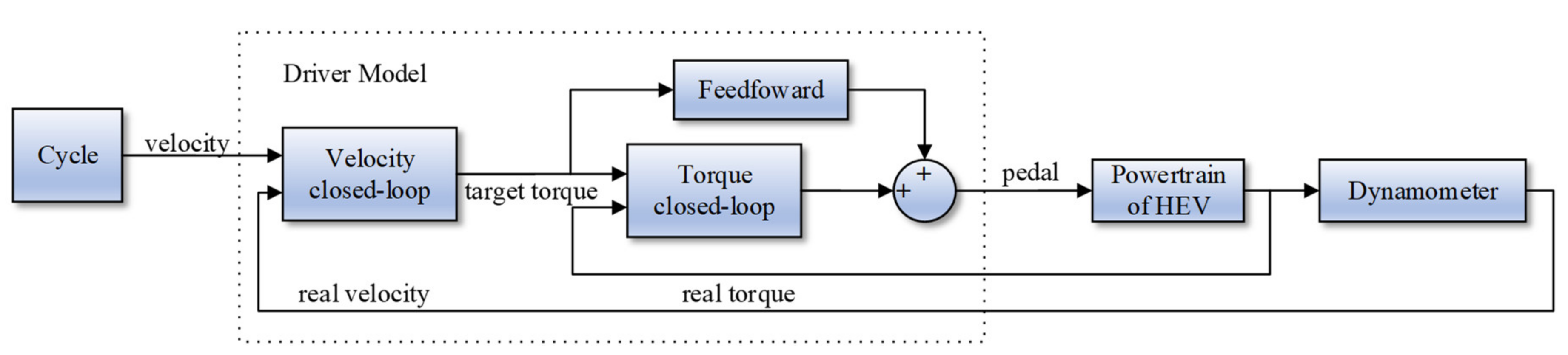
Figure 8.
The simulation platform developed based on MATLAB/Simulink.
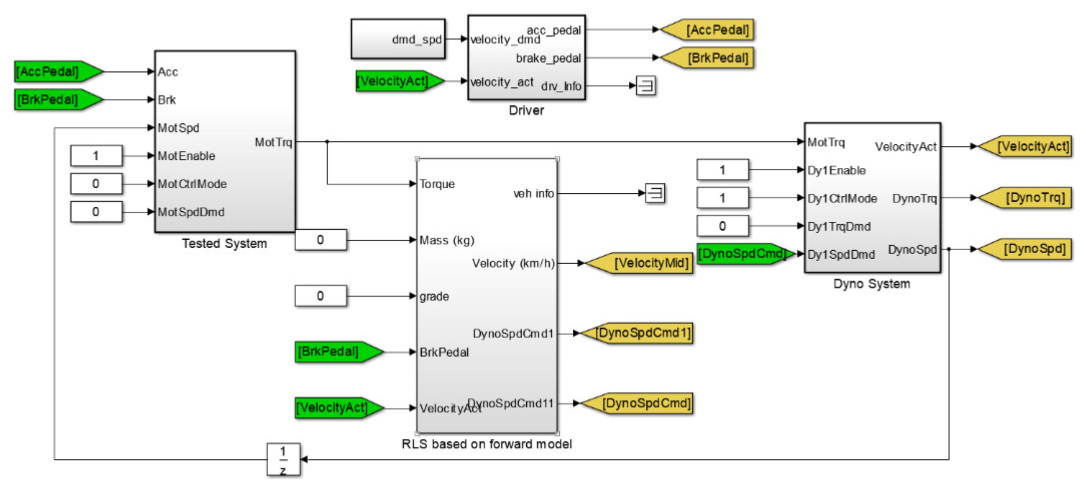
Figure 9.
The target velocity and actual velocity.
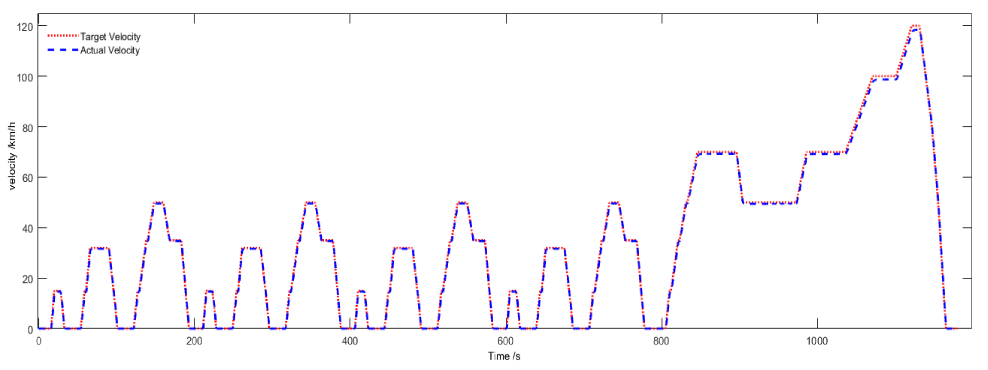
Figure 10.
The target rotation speed and actual rotation speed.
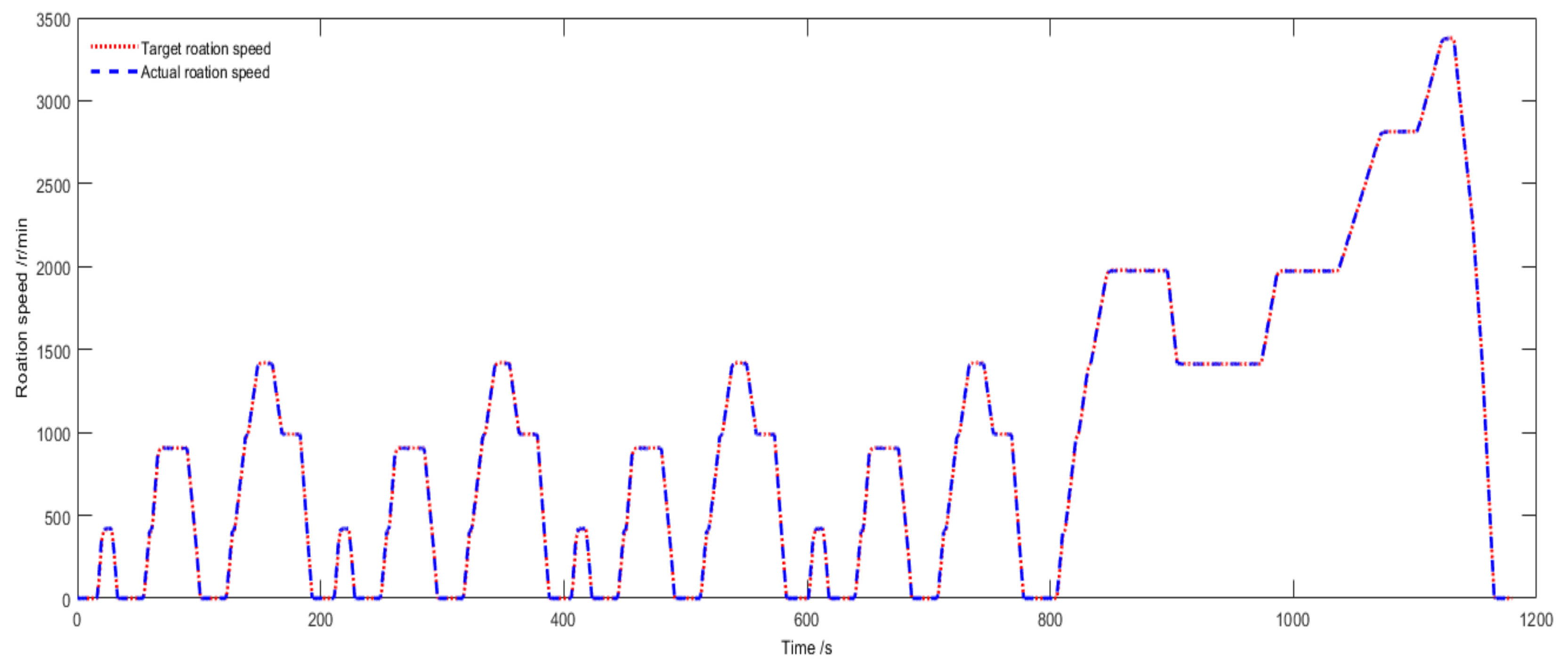
Figure 11.
The theoretical resistance torque and drive motor torque.
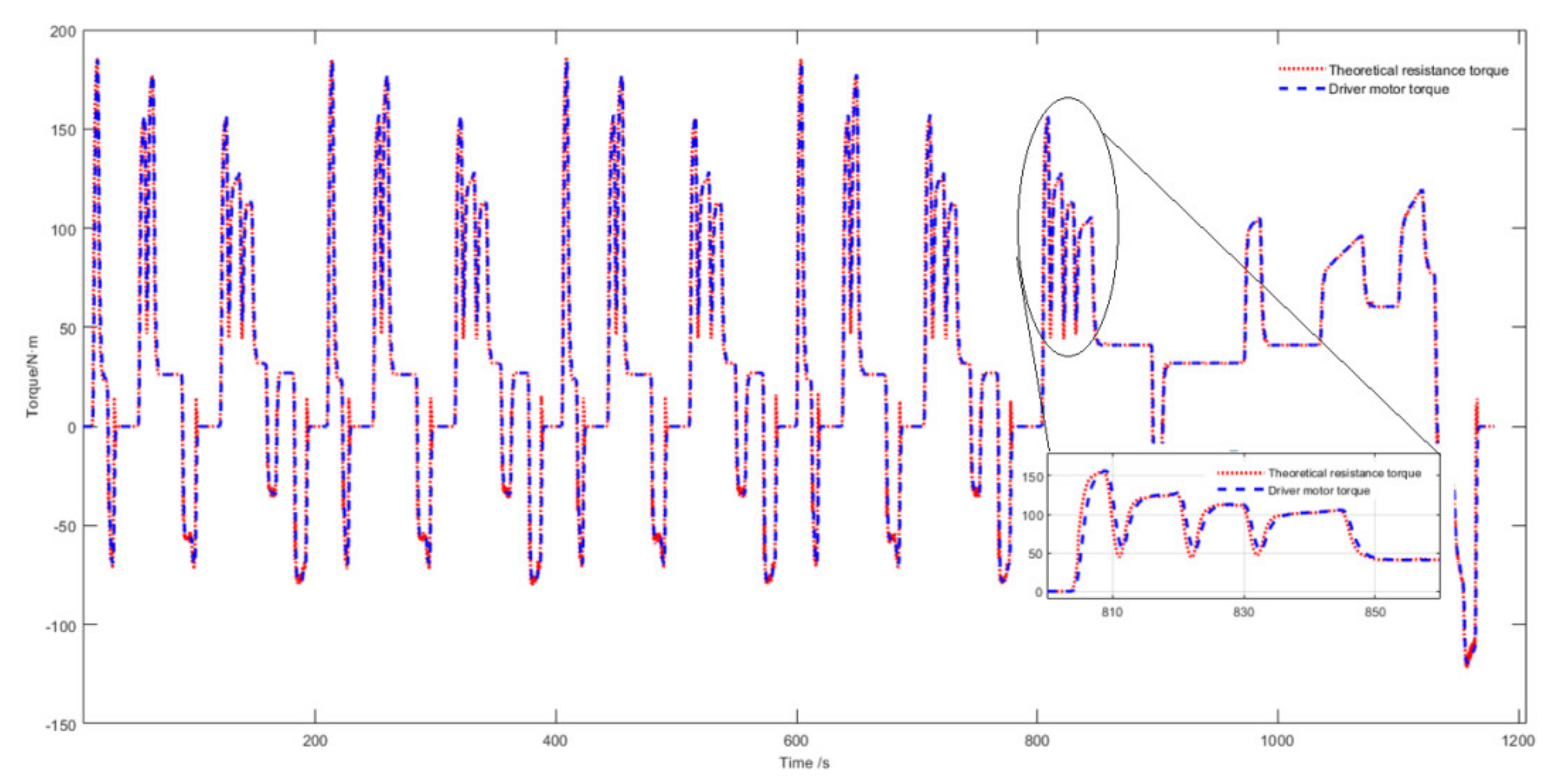
Figure 12.
Simulation results of test-beds with different inertia: (a)with the penalty function when the inertia is ; (b)without the penalty when the inertia is ; (c)without the penalty function when the inertia is ; (d) without the penalty function when the inertia is
Figure 12.
Simulation results of test-beds with different inertia: (a)with the penalty function when the inertia is ; (b)without the penalty when the inertia is ; (c)without the penalty function when the inertia is ; (d) without the penalty function when the inertia is
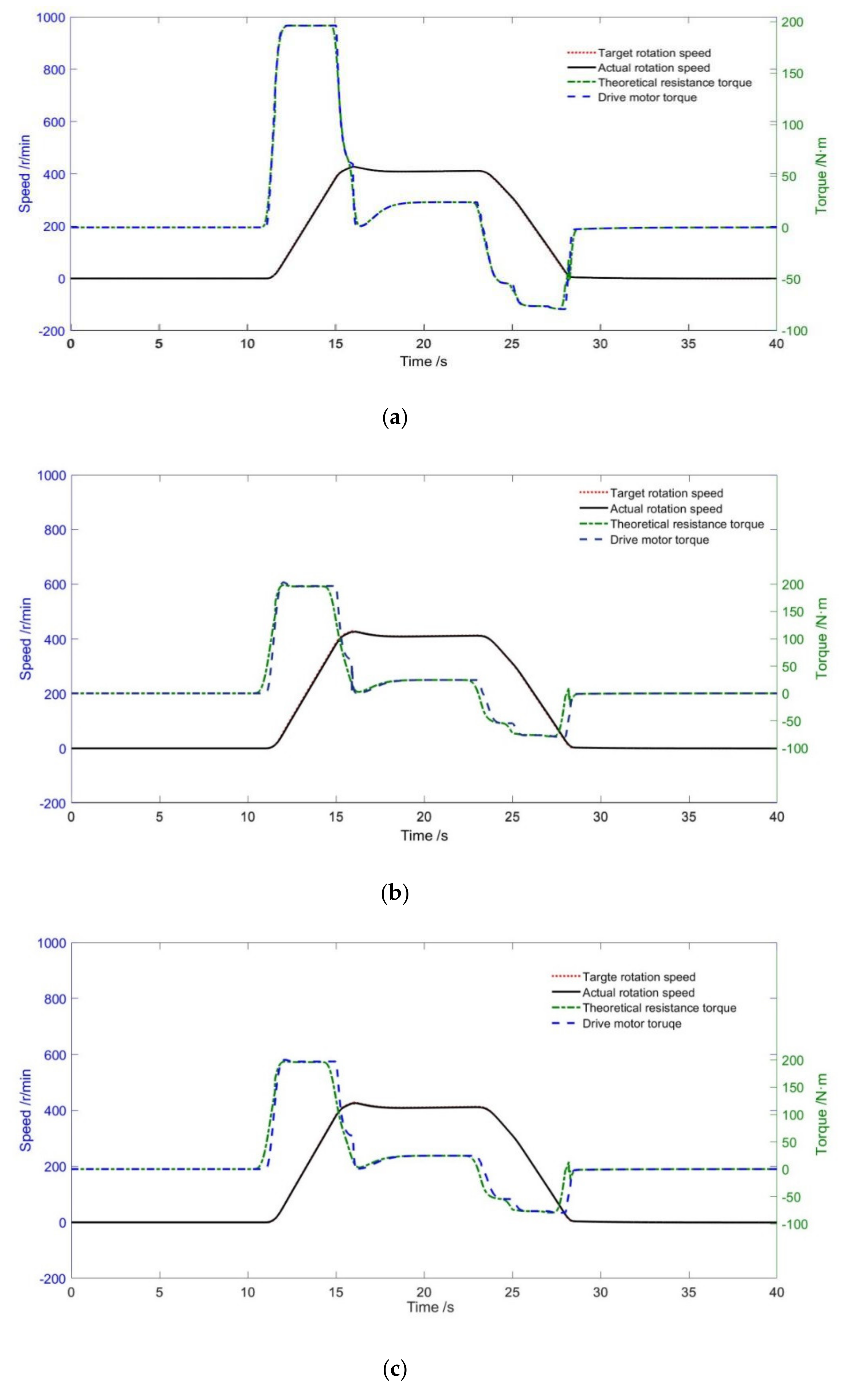
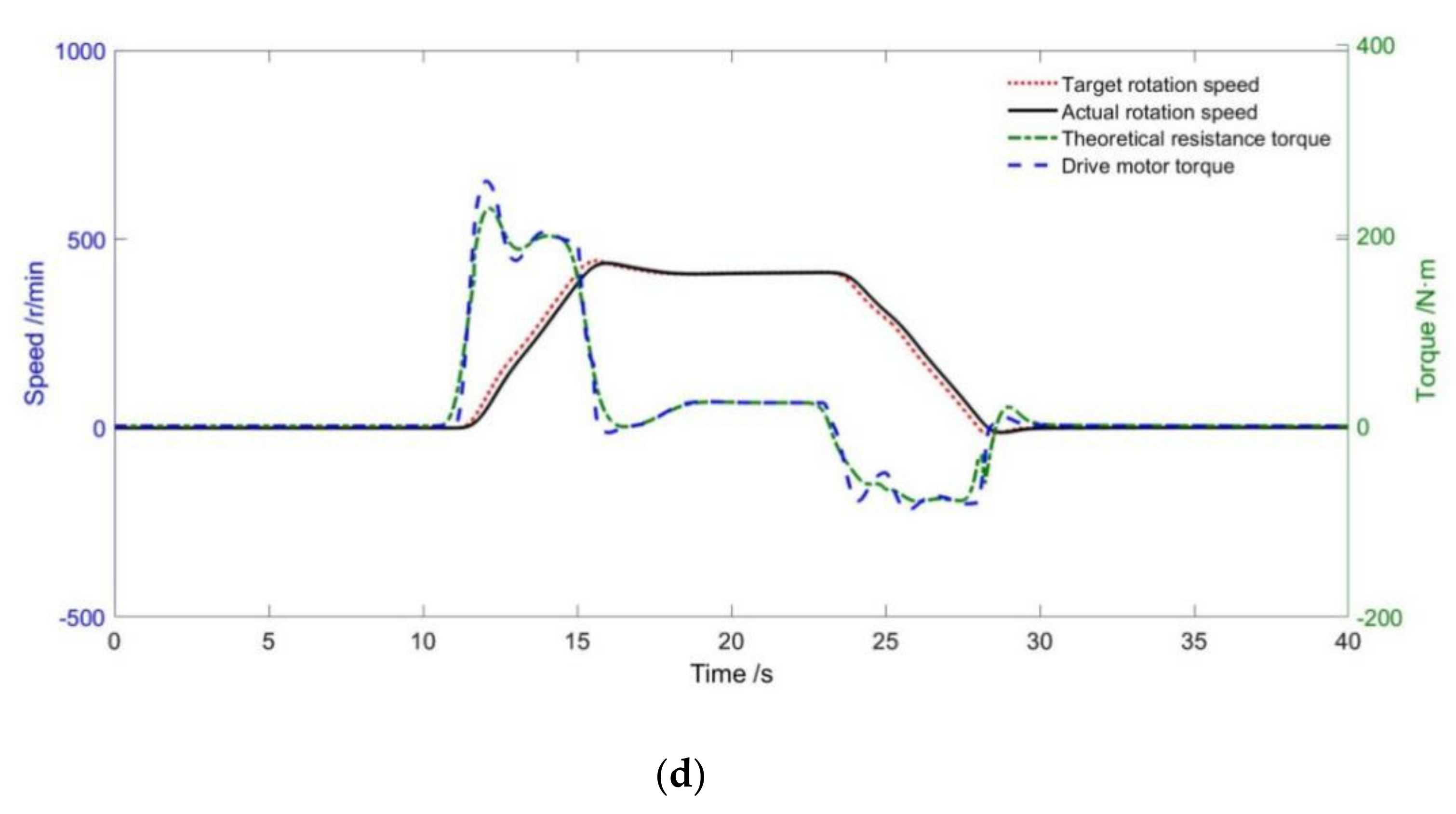
Figure 13.
Simulation results of RLS with different sampling frequencies: (a) with penalty function when the sampling frequency is 10 Hz; (b) with penalty function when the sampling frequency is 1 Hz; (c) without penalty function when the sampling frequency is 100 Hz.
Figure 13.
Simulation results of RLS with different sampling frequencies: (a) with penalty function when the sampling frequency is 10 Hz; (b) with penalty function when the sampling frequency is 1 Hz; (c) without penalty function when the sampling frequency is 100 Hz.
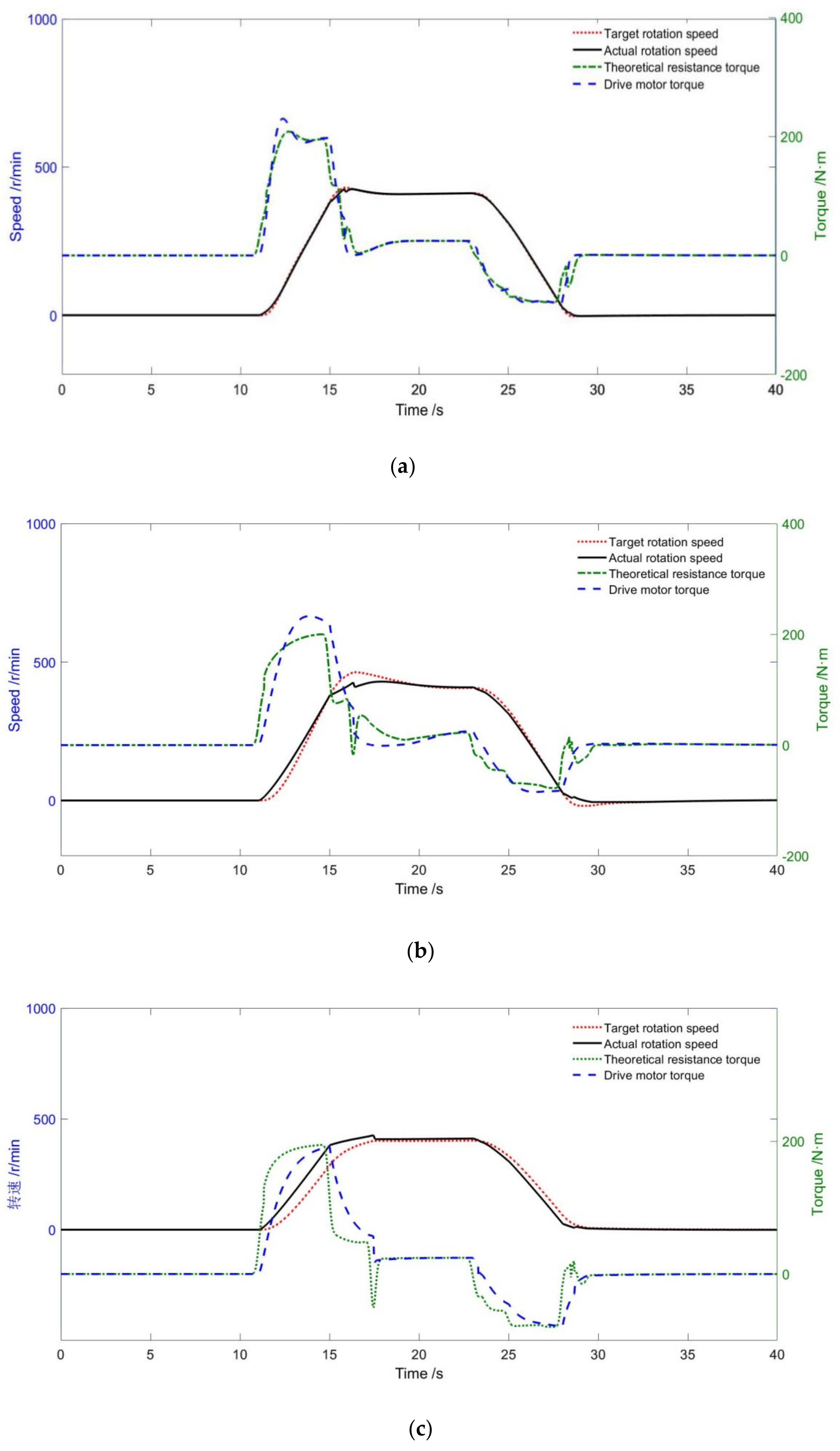
Figure 14.
Algorithm of engine simulation.
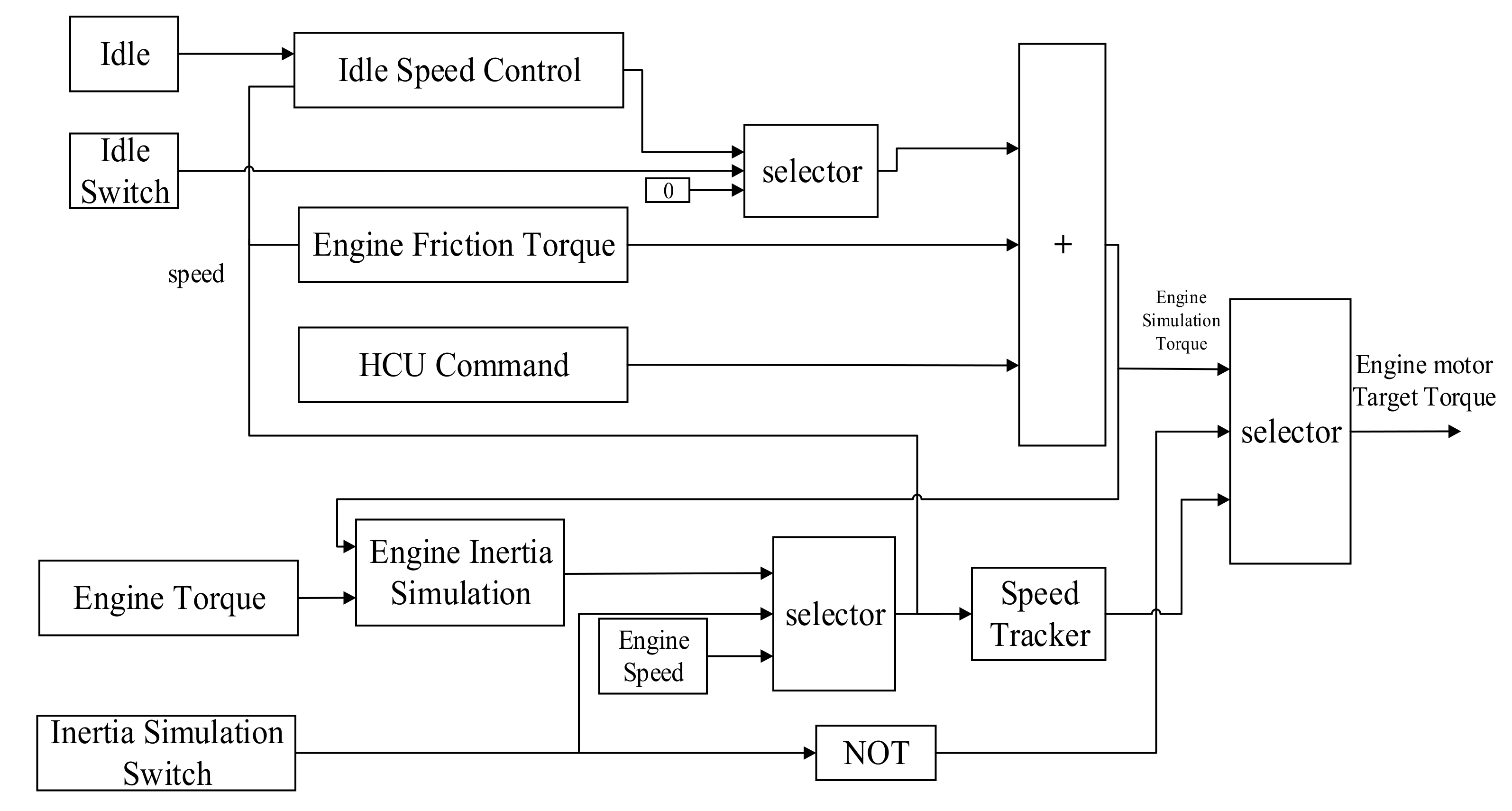
Figure 15.
Engine model developed based on MATLAB/Simulink.
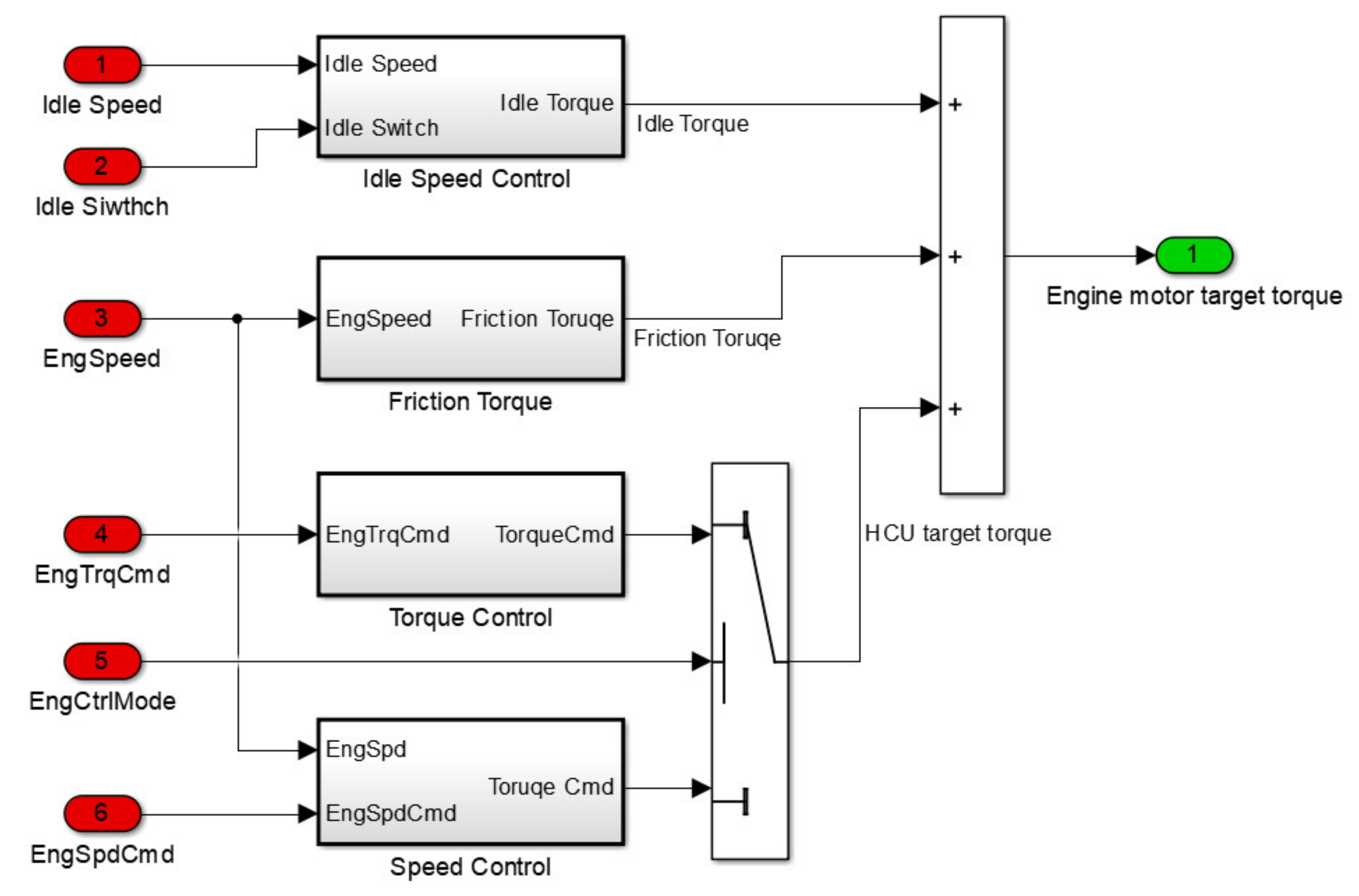
Figure 16.
Test bench for the single-axis parallel hybrid system.
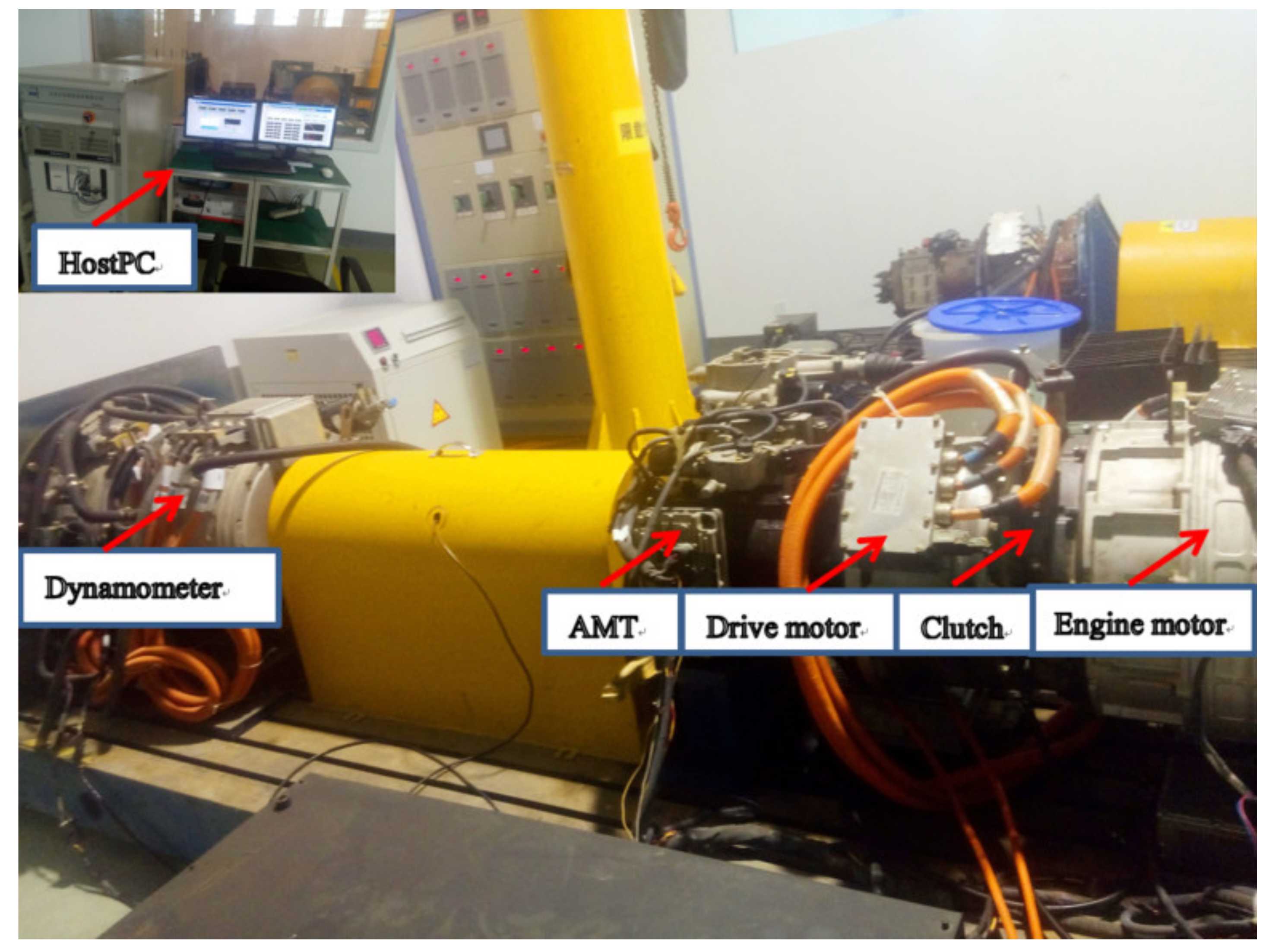
Figure 17.
Curve of the experiment: (a) Pedal and (b) Velocity.
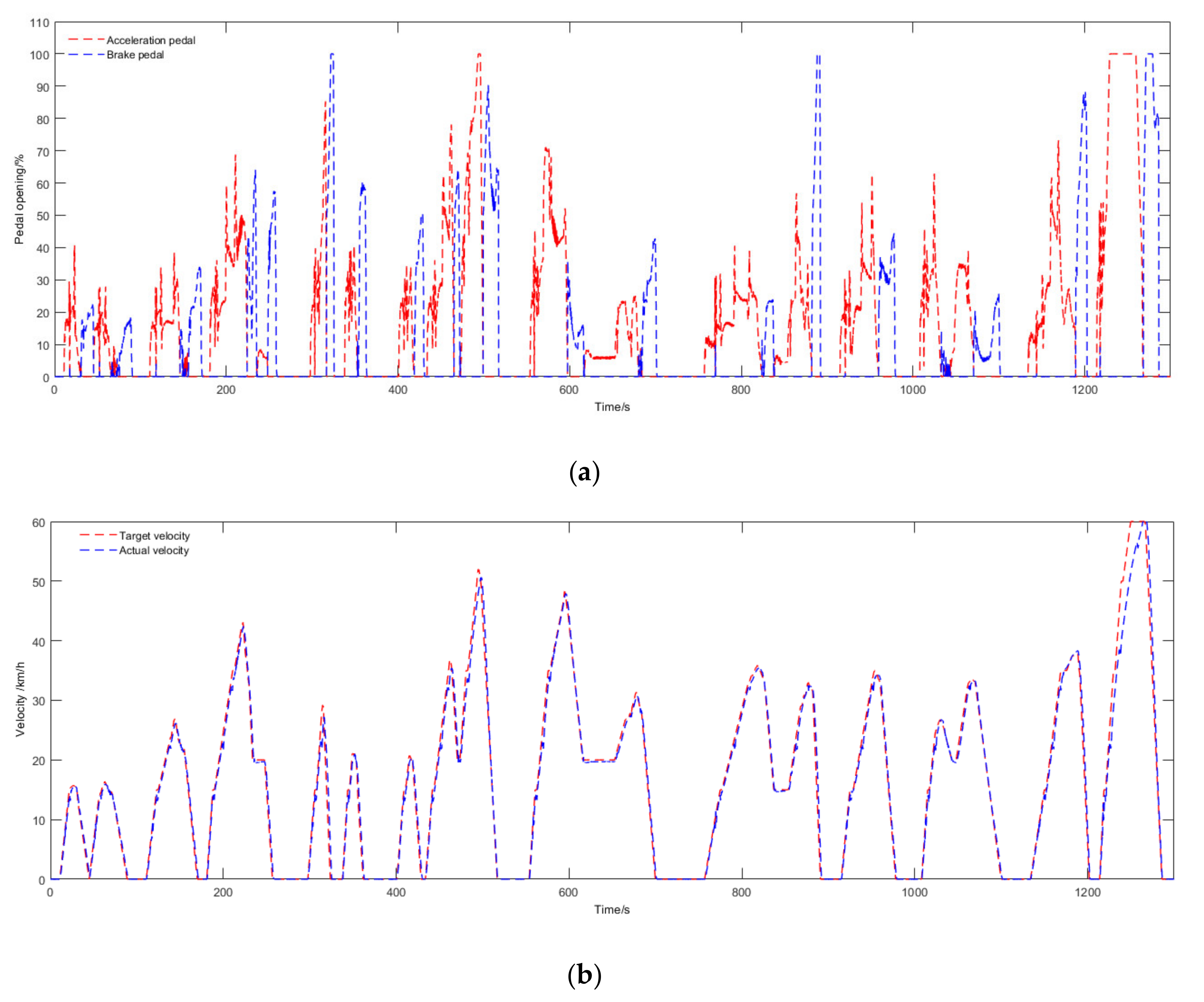
Figure 18.
The torque of engine, motor, and dynamometer.

Figure 19.
Curve of the powertrain: (a) Rotation speed and (b) Torque.
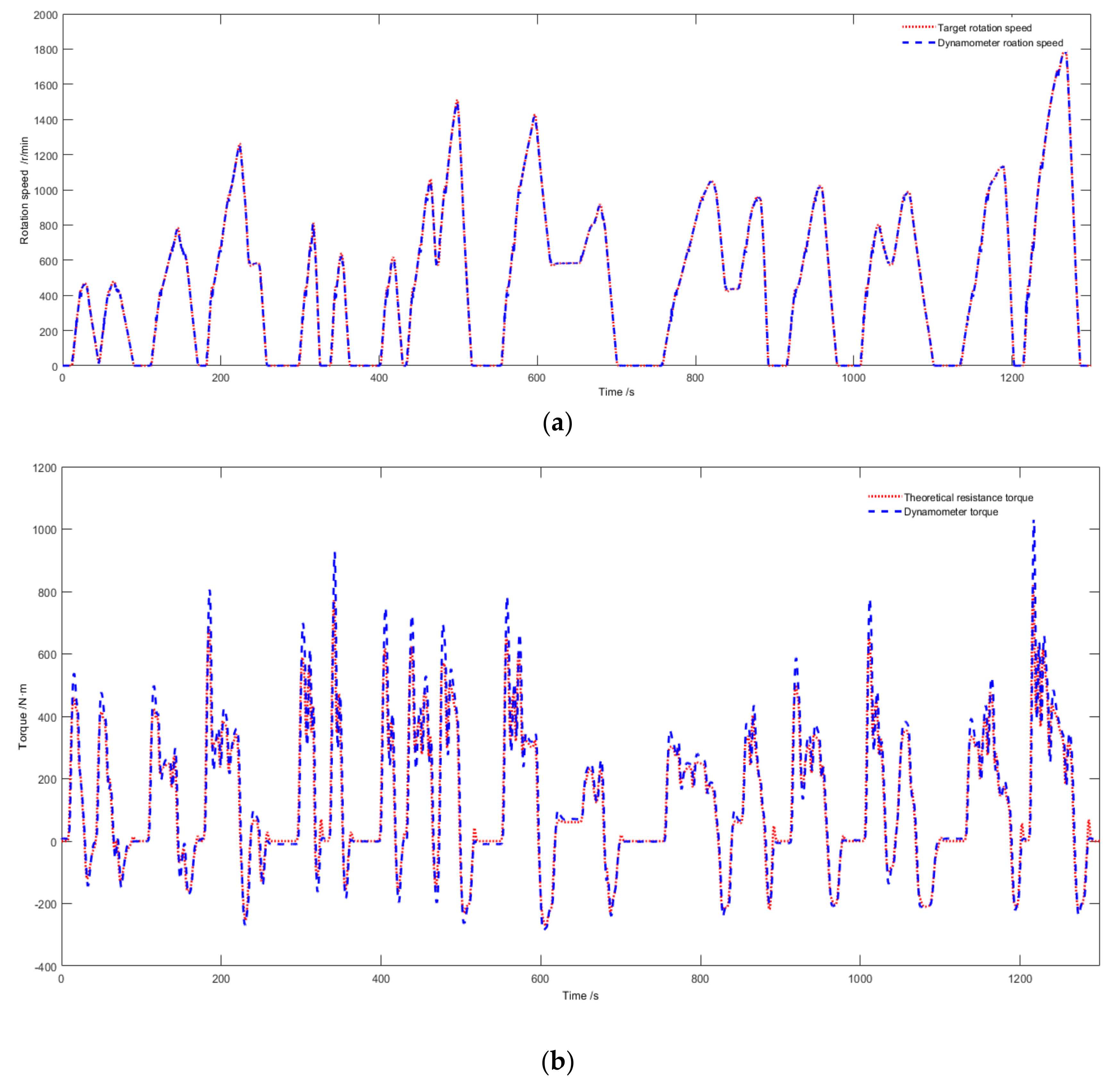
Figure 20.
The process of start and stop of engine simulation.

Figure 21.
Process of the engine simulation operation.

Table 1.
Parameters of vehicle and test-bed.
| Name of Parameters | Values | |
|---|---|---|
| Vehicle | 1745 | |
| 4.35 | ||
| 0.012 | ||
| 2.34 | ||
| 0.38 | ||
| 0.4046 | ||
| Test-bed | Rotational inertia | 0.5 |
| Rotational damping | 0.05 | |
| Maximum mechanical | 1500 | |
| 0.01 | ||
| 0.02 |
Table 2.
Simulation results comparison under the New European Driving Cycle (NEDC) cycle.
| RLS | Inertia | Maximum Torque Difference () | Maximum Speed Difference () |
|---|---|---|---|
| With the penalty function | 0.5 | 15 | 2.2 |
| Without the penalty function | 0.1 | 20 | 3.5 |
| 0.5 | 30 | 4 | |
| 5 | 40 | 20 |
Table 3.
The influence of on RLS with different sampling frequencies.
| Sample Frequencies | Maximum Torque Difference () | Maximum Speed Difference () |
| 100 | 2.2 | 15 |
| 10 | 4 | 30 |
| 1 | 5 | 50 |
| 100 without a penalty function | 7 | 60 |
Table 4.
Parameters of single-axis parallel hybrid bus.
| Name of Parameters | Values | |
|---|---|---|
| Vehicle mass | 12,000 | kg |
| Final reduction gear ratio | 5.7 | - |
| Rolling resistance coefficient | 0.014 | - |
| Frontal area | 8.25 | m2 |
| Aerodynamic drag coefficient | 0.6 | - |
| The radius of wheels | 0.5 | m |
© 2020 by the authors. Licensee MDPI, Basel, Switzerland. This article is an open access article distributed under the terms and conditions of the Creative Commons Attribution (CC BY) license (http://creativecommons.org/licenses/by/4.0/).
Share and Cite
MDPI and ACS Style
Liu, P.; Jin, Z.; Hua, Y.; Zhang, L. Development of Test-Bed Controller for Powertrain of HEV. Energies 2020, 13, 3372. https://doi.org/10.3390/en13133372
AMA Style
Liu P, Jin Z, Hua Y, Zhang L. Development of Test-Bed Controller for Powertrain of HEV. Energies. 2020; 13(13):3372. https://doi.org/10.3390/en13133372
Chicago/Turabian StyleLiu, Peng, Zhenhua Jin, Yuwei Hua, and Lu Zhang. 2020. "Development of Test-Bed Controller for Powertrain of HEV" Energies 13, no. 13: 3372. https://doi.org/10.3390/en13133372
Note that from the first issue of 2016, this journal uses article numbers instead of page numbers. See further details here.