Lifetime Modelling Issues of Power Light Emitting Diodes


Department of Electron Devices, Budapest University of Technology and Economics, 1117 Budapest, Hungary
*
Author to whom correspondence should be addressed.
Energies 2020, 13(13), 3370; https://doi.org/10.3390/en13133370
Submission received: 27 May 2020
/
Revised: 22 June 2020
/
Accepted: 23 June 2020
/
Published: 1 July 2020
(This article belongs to the Special Issue Thermal and Electro-thermal System Simulation 2020)
Abstract
:The advantages of light emitting diodes (LEDs) over previous light sources and their continuous spread in lighting applications is now indisputable. Still, proper modelling of their lifespan offers additional design possibilities, enhanced reliability, and additional energy-saving opportunities. Accurate and rapid multi-physics system level simulations could be performed in Spice compatible environments, revealing the optical, electrical and even the thermal operating parameters, provided, that the compact thermal model of the prevailing luminaire and the appropriate elapsed lifetime dependent multi-domain models of the applied LEDs are available. The work described in this article takes steps in this direction in by extending an existing multi-domain LED model in order to simulate the major effect of the elapsed operating time of LEDs used. Our approach is based on the LM-80-08 testing method, supplemented by additional specific thermal measurements. A detailed description of the TM-21-11 type extrapolation method is provided in this paper along with an extensive overview of the possible aging models that could be used for practice-oriented LED lifetime estimations.
1. Introduction
The typical failure mode of LEDs, unlike fluorescent and incandescent light sources, is not catastrophic failure. The total luminous flux of solid state light sources (SSL) experiences a continuous decrease with the elapsed operating time. The most commonly applied end-of-life criterion of LEDs is related to this constantly declining nature. The most apparent manifestation of LED aging is the luminous flux decrease, or seen from another perspective, to what extent the initial value of the emitted total luminous flux of an LED package is maintained. (sloppy, every day terminology to denote this property of LEDs is called ‘lumen maintenance’ that we shall rigorously refrain from using; instead, we shall refer to this LED property as ‘luminous flux maintenance’.) The IES LM-80 family of test methods have been developed and used in the SSL industry to measure LEDs’ luminous flux maintenance. The experiment part of our work presented here is based partly on the provisions of the IES LM-80-08 test method [1]. Besides luminous flux measurements, measuring the continuously shifting forward voltage may be part of the life tests but it is still not required in LM-80 tests and therefore such measurements or the results reporting is often omitted. In addition, LM-80-08 (like any other common life testing method) is defined at predetermined ambient temperatures and does not consider any change in the dissipated power or the degradation of the heat flow path, i.e., the cooling capability of the LED, though such tests were already proposed as early as 2011 [2]. The maximum allowed depreciation of the total luminous flux depends on the exact field of the application; the end of the SSL product lifetime is considered to be at the time when its light output deteriorates to the critical value. If an LED-based light source operates with a fixed, constant drive current, its value shall be determined so that the level of illumination remains sufficient even at the critical light output level. This results in higher illumination than necessary during most of the life cycle, as well as a significant amount of extra energy consumption. A smart controlling scheme that keeps the light output at a constant level throughout the lifetime can therefore not only increase the visual comfort of the SSL product but also improves its luminous efficiency [3,4]. Some SSL vendors already provide LED drivers that can be pre-scheduled; by gradually increasing the forward current of the LEDs, effects of the continuous total luminous flux degradation can be compensated. The elapsed lifetime dependent controlling scheme is defined for each configuration that consists of the driver, the applied heatsink and LEDs etc. The available CLO solutions most probably rely on extensive life testing results, however, the exact technical details (above the theory of the approved lifetime testing and extrapolating methods) are not put to public.
The recent industrial trends are continuously pushing product development under digitalization to reduce time-to-market and development cost. This mostly means system level computer aided simulations with the so-called digital twins (computer simulation models) of the real life components, like light sources, optical parts, heatsinks etc. Power LED modelling is still an active research area; a recent European H2020 project on LED characterization and modelling (Delphi4LED) [5] undertook to fulfil the growing industrial needs and aimed to generate the measured-data based digital twins of power LEDs [6,7,8,9]. Besides many considerations like round-robin testing [10], product variability analysis [11,12,13], chip-on-board device modelling [14] etc., one could rise the question: how could the electrical, optical and thermal parameter degradation of the LEDs be modelled? There are several analytical models for different stress conditions and parameter changes, e.g., mechanical stresses of the wire bonds [15], termo-hygro-mechanical stresses inside the package [16], shift of parameters in the Shockley diode equation [17], the course and effects of electro migration [18,19], etc.
Our present work originates also from the Delphi4LED in two ways. On the one hand, the models developed (e.g., [7]) and the test methods (see e.g., [10]) used in that project have also been used in this work. On the other hand, we focused on mainstream LEDs of today’s SSL industry (operating in the visible range) that were also the subject of investigation in Delphi4LED and in terms of classifying these devices as ‘mid-power’ or ‘high-power’, we use the same terminology that was also been used within Delphi4LED [9]. This also explains why in our study we did not consider novel LED structures or recent LEDs aimed for the display industry, despite the fact that top level publications on these devices also share significant amount of test data [20,21,22,23]; rather, we re-used some of our own archived data measured during earlier European collaborative R&D projects such as NANOTHERM [24] and we also used our own test data obtained recently.
Reliability testing and investigation of LEDs has long been a hot topic, just some examples are papers [25,26,27,28,29,30,31,32,33,34,35,36,37,38,39,40]. Still, there is a lack of a lifetime-lasting multi-physical digital pair of the already existing and widely used solid state lighting solutions, not to mention the novel devices in the research phase such as the LEDs described in papers [20,21,22,23]. This exceeded the goals of the aforementioned H2020 research project but the solution of this issue is of an increasing interest as it offers many new options in certain LED applications. The capability of modelling the parameter degradation under different environmental conditions allows to determine the controlling scheme that results in constant light output (CLO). Furthermore, accurate system level lifetime simulations could give appropriate feedback to the luminaire designers by the means of the operational pn-junction temperatures and the suitability of the cooling assembly. These altogether could provide improved reliability, lower power consumption and higher visual comfort during the whole lifetime of streetlighting luminaires.
Our initial concepts and the summary of some of our test data were provided in our prior conference publications [3,4]. In [3] the concept of stabilizing the total emitted luminous flux of LEDs for their foreseen total expected life-span was presented. In [4] actual test data were provided along with our first attempt to extend one of the multi-domain chip level LED models of the Delphi4LED project [7] with the elapsed LED lifetime. The work described in this article is a comprehensive extension of our theory and test data already presented at the THERMINIC workshops in the previous years [3,4].
2. Total Luminous Flux Maintenance Projections
Reliability and lifetime testing of electrical components is quite a diverse field of research. Due to the complex use of materials in the LED package, various types of the failure mechanisms are induced by the different ambient stress conditions, such as extremely low or high humidity and temperature or high speed change of these, off/on power switching etc. [28,29,30,31,32,33,34]. Depending on the field of application, the industry may require a wide range of various reliability tests from the light source manufacturers; to reduce the total testing time it is a common practice to accelerate the degradation mechanisms by increasing the test conditions. The so-called accelerated life tests are based on the Arrhenius model that is used to predict the aging progress under varying degrees of the environmental stress conditions. It is worth mentioning however, that besides the standard laboratory reliability tests widely used in the SSL industry, there are a couple of academic studies about possible new in-field, in-situ test methods aimed primarily for health monitoring, such as identification of LEDs’ junction temperature form their emission spectra [35,36,37] or from changes of certain diode model parameters [38], or from certain dynamic operating characteristics such as the small-signal impedance, non-zero intercept frequency or the optical modulation bandwidth [39,40].
As our work is strongly related to our prior, SSL industry inspired projects, in terms of the considered test methods we aimed to stay as close to the already standardized methods as possible. These are recommendations, approved testing methods and standards, like the IES LM-80-08 and the JESD 22-A family of standards from JEDEC [41,42]. These documents contain requirements on the measurement devices, and specify the needed test conditions like the temperature and humidity [41], change of the stress conditions with time [42], as well as the needed accuracy level of the performed measurements and the set stress parameters [1] etc.
In LED-based lighting applications the main source of any lifetime approximation is provided by the IES LM-80-08 approved method and the IES TM-21-11 technical memorandum [43]. The work described in this paper is also based on these documents. Therefore, first we would like to provide a detailed insight to show the methodology and the roots of our concept.
2.1. IES LM-80
The IES LM-80-08 description does not provide detailed instructions on the proper sample size or the sample selection, it only states that the samples under test should adequately represent the overall population. It specifies the necessary case temperatures of 55 °C and 85 °C while the value of the third testing temperature is left to the choice of the manufacturer. The tolerance of the testing case temperatures is 2 °C during the burning time, and the temperature of the surrounding air in the chamber should remain within the ±5 °C range, which should be continuously monitored by a thermocouple measurement system. The relative humidity level is prescribed to be under 65%.
Duration of the life test should be documented at least with 0.5% accuracy and also the length of any possible power failure should be considered. The optical measurements have to be measured at least at every 1000 h, while the LEDs should be driven by the aging forward current and the ambient (or heatsink) temperature should be 25 °C ± 2 °C. The total length of the test should be at least 6000 h but it is preferred to reach the total time of 10,000 h. At each photometric measurement interval chromaticity shift should be measured, as well as any possible catastrophic failure of the samples should be monitored and recorded.
The LM-80 method also gives a recommendation on the format and content of the measurement report generated at the end of the life test. Nevertheless, it does not provide provisions to qualify the LED samples and does not state anything about their lifetimes, it provides a procedure only for the measurement of the total luminous flux maintenance.
In 2015 IES published the LM-80-15 approved method [44] which is the revision of LM-80-08. In the new version there are additional requirements towards the optical and colorimetric measurements, but the prescribed three case temperatures have been reduced to only two and even the minimum test duration of 6000 h has been abolished. Regarding our LED modelling concepts the extra colorimetric measurements are not that necessary at this stage while it is still advantageous to keep the 3 case temperatures, therefore, all of our aging tests were still based on the LM-80-08 document [1].
2.2. IES TM-21-11
The IES TM-21-11 technical memorandum provides a lifetime estimation method to the measurement results of the LM-80-08 testing. The November/December 2011 issue of LEDs Magazine provides a good overview [45] on the extrapolation method.
The extrapolation technique applied by the TM-21-11 method is based on exponential curve fittings to the measured optical data of the LM-80 test. Each case temperature is approximated individually in between which the Arrhenius-equation may be used for interpolations. The recommended sample size is established by 20 packaged LEDs (either on PCB or without it). 30 or more samples would not considerably improve the estimation capability, but there is an uncertainty of extrapolations based on test results of only 10 LEDs. Within this range the number of the samples also sets the limit to the time projection; below 10 tested LEDs the extrapolation method should not be applied, up to 19 tested pieces the document allows a 5.5 times while from 20 samples it admits a 6 times extrapolation of the total test duration. The amount of the measured data used for the exponential curve fitting depends on the total test duration: collected data of the last 5k hours is taken into account up to 10k hours of aging, above that data of the last half of the test is used.
The end of operating lifetime is then defined according to the LM-80 and the TM-21 results. If the pre-defined light output degradation cannot be reached within the extrapolation limit then the result is the maximum extrapolation time itself marked with a “less-than” sign (e.g., “L70 (10k) > 55,000 h” where the “10k” denotes that the LM-80 test lasted for 10,000 h and the 5.5 times rule is applied). If the life output degradation is reached using the TM-21 estimation then the result is reported with an “equals” sign. If the samples reach the minimum light output level during the LM-80 test then the result equals to the testing time in the general reporting formula (e.g., “L90 (5k) = 5100 h”).
2.3. The Degradation Model Used by TM-21-11
The TM-21-11 technical memorandum applies an exponential curve fitting method to extrapolate the measured data in time and the Arrhenius-equation to interpolate between the three different case temperatures. The idea behind these techniques is well described in chemistry; in the following part we will use some of the basic concepts of reaction kinetics in order to give an analytical description of the LED degradation models. Our intention was to build-up and cover the fundamentals for the derivations in the later sections in the lack of such a textbook. The textbook-like manner not only introduces our efforts but also aims to provide a reliable baseline for researchers aiming to build on our work.
Reaction rate of a first-order reaction depends linearly on the reactant concentration [46]. The differential form of the rate law is:
where is the changing reactant concentration, is the elapsed time and is the reaction rate coefficient. The separable differential equation can be solved by rearranging it and integrating both sides of the following equation:
where is the initial concentration and is the initial time instant. The integration should be performed with the condition of = 0 s. After rearranging the achieved formula the rules of logarithm shall be applied. Finally, the integral form of the rate law is:
Considering the total luminous flux as the decreasing quantity of the homogenous aging process, where the initial value of the regression curve fit to the luminous flux is and is the actual value at time , then the TM-21-11 defined extrapolation of the total luminous flux maintenance curve is obtained:
where the normalized light output is at the time , is a fitting parameter and α corresponds to the reaction rate coefficient specified at Equation (1).
Homogeneous chemical processes proceeding in the solid phase involves various aging phenomena in plastic and glass, thermal changes induced transformations, recrystallization, transformation of alloys and metals throughout and following a thermal treatment etc. In the solid state these progresses need a lot more time than in gas or in liquid phase. The reaction rate coefficient (i.e., the speed of these reactions) is an exponential function of the absolute temperature. The exact formula is described by the Arrhenius-Equation:
where is a pre-exponential factor, is the activation energy (the energy barrier below which the reaction in question does not proceed), is Boltzmann’s constant and is the absolute temperature in kelvins. Concerning the TM-21 interpolations, values of and can be calculated if datasets of two or more temperatures are available.
The Arrhenius-equation is typically used to express the acceleration factor of the reaction rate coefficient at elevated temperatures:
where is the elevated temperature.
Upon taking into account the speeding-up effect of higher temperatures, the Arrhenius-equation has various expansions describing the effects of other stress conditions as well, like humidity or other non-thermal stresses. In case of LEDs, with respect to the LM-80 testing the most important non-thermal impact corresponds to the forward current [47]. The forward current dependent reaction rate coefficient can be described as:
where is the forward current and is the so called life-stressor slope [47]. With the help of Equation (7) one can perform the necessary interpolations between the measurement results belonging to the different case temperatures and forward current values captured during an LM-80 life testing of LEDs.
2.4. Further Possible Degradation Trends
The exponential decay of the total luminous flux output of an LED corresponds to the first-order reaction rate. The order of a reaction defines the relationship between the reaction rate (or the decay rate, in this case) and the changing concentration of the reactant(s) (or the decreasing total luminous flux, in this case). Practically, the order of a rate law is the sum of the exponents of the changing parameters. Accordingly, the reaction rates of the zero-, first- and second-order reactions are as follows:
For the sake of curiosity, a third-order reaction rate with two concentrations of species looks like:
where and are the concentrations of the two different species (note that the upper indices indicate the order of the reaction while the lower indices refer to the different species). To get the integral form of the above rate laws, the same mathematical steps should be followed as described in case of Equations (1)–(3).
The reaction in which one chemical species is irreversibly transformed into more than one other species is the so called parallel reaction (see also other more complex reactions in [48]). In this case the rates of the parallel reactions add up. Supposing a zero- and a first-order parallel reaction with the coefficients of and respectively, the decay rate can be written as:
The separable differential equation can be solved by rearranging it and integrating both sides of the following equation:
Rearranging Equation (14) and applying the logarithm rules, we get:
where we know that all terms are positive. Raising both sides of the equation to the power equal to the base of natural logarithm and further rearranging it we get a final version as follows:
where and are the concentration values at the time instants and , respectively. In case of LEDs, a description with parallel reactions should be appropriate when the root causes of the light output degradation can be separated. That is, for example, if the packaged blue LED, the light conversion phosphor material and the lens are aged and tested separately. These aging modes independently reduce the light output of the LED (by the means of decreasing radiant and light conversion efficiencies and light transmission), therefore, theoretically a parallel reaction model with the individual reaction rate coefficients and modes could be matched with the aging results of the complete white LED.
At the EPA ENERGY STAR Lamp Round Table held in San Diego (CA, USA) in 2011, a wider set of decay rate models describing the total luminous flux maintenance of LEDs was proposed by Miller, of the U.S. National Institute of Standards and Technology (NIST, Gaithersburg, MD, USA)—see Table 1 [49]. Among the different decay models one can find zero-, first- and second-order reaction rates, models that are inversely proportional to the elapsed time, and the parallel mixture of the previously listed ones. Miller also drew attention to the fact that the light output degradation trend of LEDs may change significantly during the operation time; Figure 1a,b indicate two relative total luminous flux maintenance curves where the estimated L70 lifetime from the 10,000-h results is halved or doubles compared to the estimation from the 6000-hour results.
3. The Pn-Junction Temperature During the LM-80 Test
The pn-junction temperature of LEDs may change significantly during an LM-80 testing procedure due to the increased electrical power consumption, to the decreased energy conversion efficiencies and even due to the possible degradation of the thermal interfaces. The temperature increase can range from only a few degrees Celsius to as high as 20–30 °C. Its exact value depends mostly on the testing forward current, the overall thermal resistance, the zero-hour radiant efficiency and on the luminous flux maintenance value reached during the test. Figure 2 shows a theoretical approximation for a high- (a) and a mid-power (b) LED, as the function of the main causes of the increase, assuming at this point, that the 3 V forward voltage and the thermal resistance remain constant. During the calculations we neglected any effects of the temperature sensitive radiant efficiency; the extremely high temperature dependence in case of red and amber LEDs is well-known and acts as a positive loopback to the junction temperature, further increasing the discussed effect.
It is obvious that a few degrees Celsius change in the junction temperature is not an issue. In this article we are dealing with the >10 °C increases caused by high testing currents, high initial efficiency, poor thermal conductivity, significant increase of the forward current and/or the thermal resistance [50,51] etc. Figure 3a,b indicate the effects of the increase in the forward voltage and in the thermal resistance. During the calculations we considered a power LED with a test current of 1 A. The initial values of the radiant efficiency, the forward voltage and the thermal resistance were 40%, 3 V and 15 K/W in order and the relative junction temperature increase was calculated as the function of the end of test thermal resistance and forward voltage. The end of test relative light output was regarded to be 95% and 80%. Stated practically, Figure 3a,b are the extensions of Figure 2a; the indicated black crosses in the figures correspond to each other. As an example for the parameter increase, Figure 4 shows the aging related forward voltage shift of a Luxeon Z power LED; all the measurement points in the figure belong to the 80 °C junction temperature.
Most of the root causes of LED aging is closely connected to the pn-junction temperature. The temperature on which the die-, the interconnection-, the phosphor- and the lens-related aging processes undergo is practically much closer to the pn-junction temperature than the case- or the soldering point temperature. Therefore, we make an attempt to determine the parameter set of the Arrhenius-equation as the function of the changing junction-temperature. To do that first we need to determine the elapsed test-time dependent function of the junction temperature.
3.1. Analytical Calculation of the Pn-Junction Temperature
The pn-junction temperature can be calculated from the ambient temperature, the optically corrected real thermal resistance and the dissipated power:
The dissipated power is the difference of the consumed electrical power and the radiant flux. For simplicity we consider to be constant over the time, therefore:
where and are the forward current and the forward voltage, while is the total radiant flux. The latter two parameters depend on the elapsed operation time t, and the actual junction-temperature and forward current. We assume an exponential decay model for the radiant flux function over time, so we apply Equations (4) and (7) and we also take into account the temperature sensitivity of the radiant flux. For simplicity we consider to be constant over the time. Therefore:
where and are the initial radiant flux and the reference operating junction temperature of the LED in the test environment at the zero-hour condition. Next, we assume a zero-order model for the increase of the forward voltage (i.e., a value linearly increasing with time) and we also consider the temperature sensitivity of the forward voltage. For simplicity we consider to be constant over the time:
After all this, the overall elapsed test-time dependent junction temperature can be written as:
which is analytically not solvable by ordinary mathematical methods. At this point we gave up with the analytical attempt and tried a measurement based practical method.
3.2. Determination of the Pn-Junction Temperature by Measurement
The strong temperature dependencies of LEDs make it necessary to measure their optical, electrical and thermal parameters simultaneously. The JEDEC JESD 51-5x family of standards and the related CIE standards [52,53,54,55,56,57,58,59,60,61] provide a multi-domain characterization method, especially for LEDs, which includes the measurement of the pn-junction temperature by the help of thermal transient testing [62,63,64] and the calibrating process of the temperature sensitive parameter, i.e., the . Of course, there are other measurement techniques (e.g., as described in [65,66]) beside the mentioned JEDEC and CIE standards/recommendations, we still work with these; over the past 15 years our research team has made significant contributions to the development of the related instruments. The gained experiences and the opportunity to customize the instrumentation also provide a higher flexibility during our investigations. In addition to these, the JEDEC JESD 51-5x family of standards is also conform with the new CIE 225:2017 recommendation and it is also used by many leading SSL companies—the reason why the Delpi4LED consortium has also chosen these standards as the basis of the LED modelling methodology also cited and described in this article.
We have performed the LM-80-08 based life testing of a mid-power LED sample set at the Department of Electron Devices of the Budapest University of Technology and Economics (see details in Section 5). Beside the optical measurements at room temperature specified by the testing method we also performed thermal transient testing both at 25 °C and at the testing case temperature. What we had after the measurements were the forward voltages, the radiant fluxes and the junction temperatures at 25 °C and at 55 °C ambient temperatures. Figure 5 shows the measured pn-junction temperatures at 300 mA forward current. Also, a linear approximation was applied on the measured results after 340 h of aging.
The temperature sensitivity of the radiant flux and the temperature sensitivity of the forward voltage can be calculated from the measurement results belonging to different junction temperatures. By having these sensitivity values it is possible to make approximate calculations for the operating parameters at any arbitrary junction temperature value.
3.3. The Transient Testing Based Calculation of the Arrhenius-Equation
The method that we propose consists of four main steps:
- (1).
- Determine the pn-junction temperature during the LM-80 process, at the test current and case temperature.
- (2).
- Determine the pre-exponential factor and the activation energy of the Arrhenius-equation from the continuously increasing junction temperature values of each measurement time and the corresponding measured radiant flux values.
- (3).
- Determine the luminous flux maintenance curve belonging to a fixed junction-temperature value, applying an arbitrary time profile of the junction temperature.
- (4).
- Determine the temperature sensitivity of the radiant flux and calculate the light output parameters at any arbitrary junction temperature and at any time of the aging process.
3.3.1. Determine the Pn-Junction Temperature
The first step was introduced in the previous subsection (see the listed references).
3.3.2. Determine the Pre-Exponential Factor and the Activation Energy
The second step is based on the LM-80 results and on the recorded junction temperature values during the test. Let us recall the differential form of the rate law (Equation (1)) and insert the Arrhenius-equation in place of the reaction rate coefficient (Equation (5)):
where and are the changing concentration and the junction temperature at the time instance of ; corresponds to (or ). Equation (22) clearly indicates the relationship between the parameters of the Arrhenius-equation and the reaction rate. Let us denote the reaction rate by (representing the fact that it is the derivative of the over function):
At any two measurement times we can write the above equations with the actual parameters:
which is a set of equations with two variables (since , and are measured values). After rearranging it we get that:
The value of can be calculated as the derivative of the experimentally acquired luminous flux maintenance curve (see Equation (4)) at the time instance of :
Although, theoretically Equations (26), (27) and (29) should unambiguously assign the values of and , still several orders of magnitudes differences may occur among the obtained results. To dissolve this issue it could be a good practice to calculate for each measurement time with an arbitrarily fixed value, then sweep until the smallest difference amongst the calculated values is reached.
Even if the junction temperature is continuously increasing during aging, its effects on the slope (i.e., the derivative) of the luminous flux maintenance curve (from which and were calculated) are negligible in most cases compared to the aging related changes of the light output parameters. Although, the following example will make it clear, that the temperature sensitivity of the optical parameters can be extremely high for red and amber LEDs. The temperature sensitivity of the radiant flux of a red power LED from a well-recognized vendor was measured to be −4.3 mW/°C at 1 A forward current whereas the optical power was found to be 1.1 W with a radiant efficiency of 41%. Mounted on a cooling assembly with a 25 K/W junction-to-ambient thermal resistance and supposing a 0.1 V and 1 K/W increase in the forward voltage and thermal resistance respectively, roughly a 7 °C increase occurs in the pn-junction temperature until the time of the 10% light output degradation, causing another thermally induced 2.8% drop in the radiant flux—which is not negligible any more. In such cases Equation (23) should be corrected in the following format:
Another possible compensation method of this effect is to determine the optical flux values that would be emitted at the reference junction temperature and use the gained data set as the new maintenance curve:
We must note, that it could seem to be a good idea to compare the values achieved by the proposed method with the results of an LM-80 test sequence performed on multiple case temperatures. In fact, the technique discussed here only makes sense if the junction temperature increase during the test is significant, but this also means that the parameters calculated from different aging case temperatures would not be well correlated with the junction temperature, therefore the latter method gives a completely different result in principle. From this reasoning we can tell that only testing at multiple case temperatures provides the needed data if the junction temperature rise is negligible, but otherwise consistent pn-junction temperature based test results can be reached only if the experiment is supported by accurate junction temperature measurements (e.g., thermal transient testing).
3.3.3. Determine the Luminous Flux Maintenance Curve at a Fixed
Our base concept is that LEDs have a kind of “lifetime budget”, which (under nominal operating conditions) is consumed at a rate most dependent on the pn-junction temperature. We model the lifetime budget as a junction temperature, forward current and elapsed operating time dependent efficiency (eta ) which is to be multiplied by the zero-hour value of the radiant efficiency or the luminous efficacy to get the prevailing light output parameters. It contains the effects of any aging phenomenon, at this point even including the change of the electrical consumption through the change of the forward voltage.
According to our theory the current value of the budget is not dependent of current value of temperature (in such a way maintaining causality). Also, it does not carry any information on the temperature sensitivity of the parameters, therefore the temperature sensitivity of the optical parameters should be applied when the junction temperature is out of the reference value. If the junction temperature remains constant during the test then the lifetime budget is identical to the luminous flux maintenance curve (described by Equation (4)) normalized to 100%.
To calculate the change of the lifetime budget (or the normalized luminous flux maintenance at the reference ) we need to recall again the differential form of the rate law. Assuming that the exact time function of the temperature change is known, we need to substitute it into:
The analytical solution of which is not trivial, even in case of a linearly changing temperature value. If the necessary mathematical tools are not available, then a practical solution could be to discretize the problem that way converting the integration to a sum calculation (a series of additions on very short time intervals). This means that the actual value of can be calculated at every time instance knowing the mean value of the temperature, then the differential form of the rate law can be used with the difference that change is calculated during the short time interval . Adding up c and will result in the total value of the next time interval.
It should be emphasized that during this step we calculated the theoretical light output parameters of the LED at the reference junction temperature but accounting for the real temperature data, which is not always equal. For example, the operating junction temperature of an LED sample is 85 °C at the 55 °C case temperature at the beginning of the test. Let us assume that after 10,000 h the operating temperature is 105 °C at the same 55 °C case temperature. In this case the value substituted into Equation (32) is the real and continuously increasing value (105 °C which is 378.15 K after 10k h) but the radiant or luminous flux provided by Equation (32) is the value the LED would emit at the reference 85 °C junction temperature. First it could be confusing but we must not forget that we calculated the pre-exponential factor and the activation energy as the function of the prevailing junction temperature (therefore the degradation itself is calculated after the aging profile). Still, these values describe only the aging effects and they do not carry any information about the temperature sensitivity of the optical parameters. If they would do so, then the method described for Equation (30) or (31) should be applied.
3.3.4. Calculating the Light Output Parameters at any
In the previous subsection we have determined the lifetime budget as the function of the elapsed lifetime and junction temperature profile in the meantime. The calculations result in the actual radiant flux value that would be emitted at the reference junction temperature, after the elapsed operating lifetime . The next step is to apply the temperature sensitivity of the radiant flux if the value increases/changes significantly during aging:
where is the zero-hour radiant flux, (eta t) is the lifetime budget number at time . The value of can be determined at zero-hour and used during the whole lifetime as a constant or it can be re-determined at each control measurement. In practice according to the proposed method thermal transient testing should be performed both at case temperature and at the LM-80 prescribed 25 °C ambient temperature. From these measurements a linear approximation of all temperature sensitivity parameters can be determined.
3.4. Case Study
The procedure suggested in Section 3.3 was performed on the measurement results of the LED sample presented in Section 3.2. The steps taken are as follows:
- (1).
- (2).
- was calculated.
- (3).
- ( = 85 °C) was calculated for all the control measurements (Equation (31); the red dots in Figure 6).
- (4).
- (5).
- and were determined; the measured values at = 55 °C and the maintenance curve determined in step 4 were used. Applying the same method described in Section 3.3.2 the formulas for the logarithmic model are:
- (1).
- To check the accuracy of the achieved model we calculated the maintenance curve belonging to TJ = 85 °C (dashed dark red line in Figure 6). The simulation run with a time increments of 1 h.
- (2).
- We also calculated the maintenance curves belonging to = 25 °C and to = 55 °C (dashed dark blue and green lines in Figure 6).
To represent the appropriateness of the proposed technique the R-square values were determined with respect to the measured data. The R2 values of the simulation are 0.992 and 0.988 for the 25 °C and 55 °C measurements while that of the logarithmic approximation are 0.993 and 0.983. These values show that the accuracy of the new aging model and the classical curve fitting method is practically the same.
Figure 6 also indicates that the simulated results and the fitted curves have different curvatures and their separation becomes quite significant after around 5000 h. Obviously, neither approximation of the measured values is more accurate than the other. The main cause of this misfit is probably the low statistical power of the measurement results of one single sample (and perhaps the changing aging rate). The purpose of this short case study was only to demonstrate the potential and feasibility of the theory.
4. LM-80 Based Lifetime Modelling of Power LEDs
Once the fitting parameters of the total luminous flux maintenance curves (and the pre-exponential factor(s) along with the activation energy (or energies)) are available, it becomes possible to estimate the in-situ light output parameters of an LED at any time (by Equations (7) and (32)), provided that the prevailing junction temperature and forward current values are always known.
In case of a streetlighting luminaire the forward current is either kept constant or it is controlled by a smart device. In fact, aging of the LED driver may cause aging related deviations in the set current but discussion of such issues is out of the scope of this article.
In-situ measurement of the pn-junction temperatures is not impossible, but it requires specialized laboratory equipment. Another solution is to reveal the operating temperature map of the luminaire can be achieved by system level simulations [67,68,69,70] that way shifting the junction temperature measurements to a predetermined point of the luminaire. System level simulations with multi-domain LED models make it possible to tell the operating parameters just by measuring the luminaire case temperature which is then on the field, mostly depends on the actual weather conditions.
4.1. Continuous In-Situ Lifetime Modelling of LEDs
Generating a time-dependent absolute temperature function from years of weather conditions is not realistic, but in the short period of time (e.g., within an hour) it can be assumed that the temperature changes linearly over the time. This approximation makes it possible to solve Equation (32) analytically, but despite of it, the computing capacity of the intelligent control unit of the luminaire may still be insufficient for the required calculations (or it is not acceptable for the unit to be kept busy by these calculations—also not counting with the power consumption of the CPU). If the value of reaction (or decay) rate coefficient is recalculated periodically at short intervals (e.g., every 5–10 min) and approximating the temperature to be constant in the meantime, then Equation (32) is greatly simplified:
where c is the actual light output value of the LED and the lower indices 1 and 2 denote the initial and the terminating time in-between the LED aging is calculated.
A case study was carried out to present the capabilities of the theory. For this purpose, the LM-80-08 based measurement results of Luxeon Z LEDs aged in our department were used (see the results in Figure 7a). The natural white high-power LEDs had a junction-to-ambient thermal resistance of 35 K/W. In Figure 7b the continuous red curve indicates the exponential fit to the measurement results (the same as the dashed orange curve in Figure 7a). Further eight theoretical aging curves were added in order to make the necessary calculations feasible, corresponding to = 85 °C and 50 °C and to = 850 mA and 700 mA.
Figure 8 shows an illustrative example of the theory, applying Equation (36): the stress conditions are abruptly changed at 30k hours of aging from = 120 °C and = 1 A to = 50 °C, = 0.85 A.
4.2. Lifetime Modelling of Iso-Flux Operation; a Case Study
By keeping the total luminous flux of solid-state light sources constant, not only the visual comfort can be improved, but the reliability and energy efficiency of the luminaires could also be greatly increased. The advantage of a design method that compensates for the effects of temperature changes has been presented in previous articles [68,69,70]. The previously proposed methodology has not yet taken into account the aging of LEDs, which in the long time range may be even more significant than the effects of temperature changes.
The total lifespan of LEDs is typically referred to be in the range of 50–100k hours. This period can be easily converted to lifetime in years for light sources that operate without interruption (e.g., tunnel lighting or lamps at industrial facilities), but in case of streetlighting luminaires the conversion is not that straightforward as the on and off time depends on the length of days that alternate continuously throughout the year. In addition, switching on and off the lights does not necessarily depend on the exact occurrence of the twilights; the operating time measured in years should be considered based on astronomical data, taking into account the changing length of the nights. Table 2 illustrates the typical practical lifetime of a luminaire (assuming a rated LED lifetime of 50k hours) in Hungary.
A case study was carried out on the real and theoretical LED aging results in order to demonstrate the range of differences between a constant current and a constant luminous flux operation. In order to count with realistic temperature variations the daily temperature values of the past decade of the Hungarian city of Szombathely (47.23512° N 16.62191° E) available at the Hungarian Meteorological Service, have been used, for which the constant current mode and the constant luminous flux operation was compared. The difference between the length of cold winter nights and warm summer nights was also considered by taking into account the annual change in the time differences between the civil twilight. At this stage we dealt with only one single LED, with the junction-to-ambient thermal resistance of 35 K/W.
The results of the case study are shown in Figure 9, Figure 10 and Figure 11: the consumed electricity can be considerably decreased, particularly in the first year of the operation which means that a significant portion of the cost of a new luminaire installation is recovered within a relatively short time. Figure 10 clearly indicates, that using the smart controlling scheme the light output can be kept constant against the effects of temperature changes in the short run as well as against the LED aging in the time scale of decades (considering only the LED light sources–any other aging effects form a different issue). Due to the more favorable operating conditions (lower forward current and junction temperature values), the expected product lifetime could also be increase significantly.
In case of the smart control that realizes constant luminous flux output throughout the whole product lifetime, it is obvious that the normalized total luminous flux maintenance percentage can hardly be used to determine the end of the product lifetime. For that purpose we propose the lifetime budget efficiency (eta ) as the new end-of-life metric for adaptively controlled LED luminaires. The final results are summarized in Table 3.
5. Lifetime Modelling Based on Multi-Domain Modelling of the LEDs
The purpose of our multi-domain LED modelling concept is the simultaneous and combined simulation of the optical, electrical and thermal operation parameters. The proposed modelling technique is continuously revised and enhanced in order to achieve higher accuracy, better industrial applicability and also to add further capabilities to the model. Significant improvements have been achieved during the Delphi4LED H2020 European R&D project and the next step shall be modelling the whole lifetime of LED based light sources by the help of a Spice compatible multi-physics model.
Multi-physics LED models are generated by the isothermal LED characteristics which consist of the electrical and optical data as a function of the forward current, measured at a fixed junction temperature. Such measurements can be performed by the help of the T3Ster and TeraLED [71,72] measuring instrument setup; to speed up the rather time-consuming characterization process the vendor also provides an automated control software to the instrumentation. Then the multi-domain LED model can be generated by a global parameter fitting process; a detailed description on the model and its variants, benefits and various properties is provided in the recently published paper in this journal [7].
Combining the existing multi-domain LED model with the measurement results of an LM-80 based life test is a promising attempt. It means that a complete isothermal characterization of the LEDs should be performed as the testing time passes, which is the main drawback of this technique, compared to the common measurement methods during life testing. Its benefit is, however, that the elapsed operating time dependent model parameters can be revealed.
5.1. Evaluation of Precious Life Testing Results
A sample set of 30 HP LEDs has already been aged under an LM-80-08 based life test, during which the measurements were also extended by the abovementioned isothermal characterization technique. In the earlier study the samples were exposed to the case temperature of 85 °C while they were driven by the forward current of 1 A. The whole test lasted for 8k hours (Figure 12a shows the normalized total radiant and luminous maintenance curves). Detailed isothermal characterization was performed in the first 6k hours on 5 LED samples from which the model parameters were determined as the function of the elapsed time (Figure 12b shows an example) [73].
In case of all the characterized samples the obtained model parameters showed high similarity, and also the time dependent trends were consistent with each other. Still, a proper elapsed lifetime dependent model could not be generated from these. The difference in the ideality factors were found to be relatively small on a linear scale, but due to the exponential form of the Shockley diode equation even very tiny misfits can cause large errors in the output electrical and optical values. Besides this, there is an inflection point at around 1k–1.5k h of aging which prevents any modelling attempts with a simple time-function of the parameters; the use of complicated complex functions would not necessary describe the real physical aging processes but it would significantly increase the difficulty and the needed time of the global parameter fitting process. It is also obvious that various aging phenomena took place in the early “burn-in” part of the LEDs’ lifetime and also their significance were changing with time; the collected data before 2.3k h of aging should be omitted during the model generation process. The appropriate time dependent model, however, cannot be created from only 3 characterization points.
5.2. Launch of a Targeted LM-80 Based Test Sequence
Instead of fixing the total testing time in advance, it could be more advantageous to pre-define a targeted total luminous flux depreciation level in order to have a better overview on the time evolution of the time evolution of the modelling parameters. Based on this idea a new LM-80 like test was conducted on 18 mid-power LED samples from a well-recognized vendor. The LED type selection was made according to our previously performed tests and detailed measurements. Testing a set of high-power LEDs would also been interesting; preparation of such tests is already underway.
The samples were exposed to the case temperatures of the specified 55 °C and 85 °C and at the arbitrarily chosen 70 °C. At each case temperature, three different forward currents were applied: 220, 260 and 300 mA, the latter one as the absolute maximum allowed forward current of this LED type (the nominal current value is 150 mA). This means only two samples per each aging condition (case temperature/forward current), which is insufficient for TM-21-11 extrapolations but the purpose of the test was much rather to support our theoretical assumptions than to collect statistical data for industrial applications and needs. During the test we did not only measure the necessary parameters prescribed by the LM-80-08 standard but we also performed a complete isothermal forward current–forward voltage–radiant flux characterization of the samples in a 500 mm integrating sphere. These captured iso I–V–L curves were expected to provide enough input data to reveal the effects of the different aging tendencies.
The tested LEDs arrived on 0.8 mm FR4 stripes that had extended thermal pads both on the top and on the bottom sides (see in Figure 13). The samples were electrically connected in series in the chains of 6 LEDs. In order to make the JEDEC JESD 51 compliant individual measurements of the samples the stripes were chopped between the LEDs. Prior to the LM-80 aging test the samples had been pre-characterized during which the radiant flux was measured to be around 50% at the nominal forward current, however, the real thermal resistance was measured to be around 100–150 K/W; from the integral structure functions it was obvious that the most significant part of it belonged to the LED package itself. The exact causes of the unexpectedly high thermal resistance values were not examined in more depth, but according to our assumptions the pre-bake technological step may have been omitted before soldering, therefore the humidity accumulated in the LED package may have caused delamination of the internal mechanical layers during the reflow process.
5.3. Results of the LM-80 Based Test
The LM-80-based investigation of the mid-power LEDs was ended after the elapsed time of 1735 h because of the high failure rate of the LEDs; till the termination of the test 14 LEDs suffered catastrophic failure and two further pieces had contact failure. The rapid and early failure of the samples was unfortunate but not unexpected; in only a few cases the testing junction temperature of the LEDs was close to the allowed maximum value, but in most cases it was far above that. Despite the fact that the testing case temperatures were specified according to the LM-80-08 description, the lifetime testing still went in an accelerated manner (reaching the L70 level was one of our goals anyway).
Figure 14 compares a faulty and an unaged sample. From the figure it can be clearly seen that one of the root causes of the failure may be traced back to the extremely high temperature around the chip that inflicted carbonization of the encapsulant material, causing discoloration and bubbling. Due to the reduced light transmission of the lens higher amount of the blue light was absorbed that further increased the self-heating effect inside the LED package. The catastrophic failure most probably occurred as a result of a thermal runaway.
Figure 15 shows the attained total radiant flux maintenance curves; the case temperatures are indicated by different colors while the different forward current values are marked with different line types. Interestingly, the LEDs exposed to the lowest case temperature not only aged faster, but the trend over the time is also different from the others. Deeper investigations were not conducted to reveal the proper reasons and phenomena, but the main reason for the differences may be the higher RH formed at the lower temperature; this assumption is also supported by a previous study of a moisture resistance test on the same LED type, presented in paper [4].
All in all unfortunately, the captured LM-80 compliant measurement data altogether did not make it possible to further analyze the temperature and forward current dependence of the aging rate. In Section 3.4 however, an attempt was made to achieve the Arrhenius equation parameters, but in this exact case there is not enough measurement result of the other two case temperatures to support our theory; the resources required for such investigations far exceed the academic capabilities.
5.4. The Elapsed Lifetime Dependent Multi-Domain LED Model
Using the obtained measurement results an attempt was made in order to investigate the lifetime modelling possibilities and the extrapolation capabilities; for this purpose the multi-domain models of the still functional #S07 and #S11 samples were created at first. Various functions were tried out during a global parameter fitting process in order to set up the lifetime LED models with the best match to the measured characteristics. For this purpose, rudimentary parameter matching software was also developed, which ran on a mid-range 4-core processor for about 1 week (which was about one-tenth of the total software development time). The obtained Shockley model parameters and the value of the series resistance have significant elapsed time dependence. An improved version of the fitting application was re-run iteratively three times in order to achieve the first attempt of our elapsed lifetime dependent multi-physics LED model; Figure 16 indicates examples of the attained model parameters.
After defining the new lifetime LED model a simulation test bench was created by which the LM-80 based test data could be compared with the modelled values (see the results in Figure 17a). The average absolute inaccuracy of the simulations is 0.5% while the maximum deviation is 1.2%. Figure 17a also shows that due to the quadratic and logarithmic time functions of the fitting parameters of the Shockley diode equation (see in Figure 16a,b) the model fits very well even in the early burn-in period—at least at the time of the measurements. Otherwise, further simulations with much higher time resolution has shown that the model becomes totally inconsistent between 1 and 100 h of aging (see in Figure 17b). These results strongly highlight the risk of using high-degree parameter matching algorithms. The extrapolation applicability of the new model still had to be tested therefore samples #S07 and #S11 were reinstated to the test chamber. In the meantime, the time functions of the fitting parameters were revised in order to eliminate the anomaly of the early aging time.
5.5. The Enhanced Time Functions
While the test continued on the two samples, we reconsidered the time functions that were previously found to provide the best match. After an extensive “trial and error” type investigation of the possibilities it was decided to apply only such functions that push the results only in the same direction while the rest of the parameters were kept constant. The biggest error in each case occurred in the initial burn-in stage, so we decided not to deal with it in the first round. That way the multi-domain model simplified remarkably: the shift of the forward voltage can be modelled by a linearly increasing series resistance, while the saturation current and the ideality factor of the electrical model are constant values. That way the electrical and the optical degradation of the LED can be modelled completely separately: the time function of the light output decay can be applied for the saturation current of the optical branch while its ideality factor and series resistance remain constant.
Considering the initial 100 h of aging, an additive exponential decay with a very short time constant describes well the forward voltage of the LED. The electrical series resistance therefore is formed this way:
where is the elapsed operation time is the zero-hour electrical series resistance, and are fitting parameters and is the time constant of the initial exponential deviation.
Regarding the radiant flux, so far no correction function was found to describe the burn-in time. The saturation current of the optical branch is therefore:
where is the zero hour saturation current of the optical branch and is a fitting parameter. According to this function the model is not applicable if < 1 h and also gives inaccurate results if < 100 h.
5.6. Extrapolation Capabilities of the Model
At 4340 h of the total aging time the two samples #S07 and #S11 were again unloaded from the aging chamber and were re-measured in our integrating sphere. The obtained measurement results (the radiant flux and the forward voltage values) are shown in Figure 18a–d along with the lifetime extrapolation simulation curves. The simulations were performed by the LED models based on the measurement results obtained up to 1000 h.
For sample #S11, the estimations acquired from the simulations are quite accurate, while the model of sample #S07 overestimates the extent of changes (see the mismatch values in Table 4). A possible explanation for the error could be the fact that the samples had to be removed from the aging environment for each measurement. Re-fixing the samples with different strengths may affect the value of thermal resistance. This possible reason is consistent with the previous assumptions that the high thermal resistance may have been caused by hygro-mechanical stresses that induced delamination of the mechanical layers in the LED packages.
It has to be noted that at this point the model is only valid for the 300 mA aging circumstances. Regarding the temperature issues, according to our theory the Arrhenius-equation parameters determined in Section 3.4 can be directly inserted into the model of #S11 sample:
by which the saturation current of the optical branch can be calculated at any time . Dealing with discretized time steps of very short intervals and considering the temperature to be constant in the meanwhile we can calculate the value of the next period:
With the same considerations it is possible to sensitize the time-dependent electrical series resistance value to the junction temperature. In case of this LED type it should be based on the zero-order model of the differential rate law.
5.7. The Required Measurement and Testing Time
In case of the LM-80-08 based life testing of the blue mid-power LED set the isothermal characterization process was optimized to the needed time: the measured set of operating points was reduced to the minimally sufficient range while the small size of the LED packages and the relatively short thermal time constants (around 30–60 s) were also advantageous to significantly speed up the measurements. In spite of these facts, the required measurement time per each sample was around 180 min at each control event. Such characterization was performed 87 times during the test which altogether amounts a total measurement time of 260 h; an additional 15% of the original 1735 h of LED aging.
The minimal LM-80-08 and TM-21-11 compliant sample set consists of 90 LEDs as the testing process prescribes three case temperatures and at least three testing currents are necessary for proper interpolations in between while the extrapolation technique may be applied in the presence of at least 10 samples per aging conditions. Supposing a typical high-power LED the full characterization time may take even up to 6–8 h which means a total measurement time of 500–700 h at every control event that (according to LM-80-08) must be performed at every 1000 h. Although the measurements could be fully parallelized, it is still not realistic for academy in terms of the price of the currently available instruments required for the isothermal LED characterization. Therefore, supporting the theory described in this paper by appropriate statistical background remains an opportunity much rather for the major industry partners. Also, reducing the necessary measurement time of the current LED characterization system could also help to put this method into common practice.
6. Conclusions
In this work the LM-80-08 and TM-21-11 documents were briefly introduced after which an extensive description of the applied decay models were provided. In addition to the models used in the accepted methods, we also presented other aging models and the mathematical basis of their application.
Applying the theoretical basics of the light output degradation of LEDs we have introduced a novel method to determine the pre-exponential factor and the activation energy of the Arrhenius-equation only by measuring a sample set of only one aging case temperature instead of the prescribed three. We have also pointed out, that consistent pn-junction temperature based test results can be reached only if the experiment is supported by accurate junction temperature measurements in cases where the junction temperature rise during the life testing is considerable. Our theory was also supported by the evaluation of real measurement results. The case study showed that the LM-80 based measurement results of a power LED sample set and our LED aging theory of the “lifetime budget” were applied in a case study based on archive meteorological data. The case study showed that the iso-flux (or constant light output) operation mode has very significant benefits in terms of both electrical consumption and lifetime expectancy.
In order to create the elapsed lifetime dependent multi-domain LED model an LM-80-08-based test was performed on 18 blue mid-power LEDs of a well-recognized vendor. During the test even the isothermal characteristics of the samples were captured. Extremely high operating junction temperature of the samples even at the prescribed case temperatures caused fast and early failure of the LEDs. The speed and the trends of the LED aging also showed significant anomalies: the highest aging rate belonged to the samples of the lowest test temperature and even their total luminous flux maintenance curves follow a logarithmic trend instead of the expected exponential one. In the absence of the sufficient aging data ant due to the experienced anomalies it was not possible to determine the forward current dependent LED aging model but a theory was set up to specify the Arrhenius equation’s parameters from only one testing temperature, by the help of thermal transient testing. In this specific case the needed extra measurements of the proposed method added a 15% surplus to the life testing duration which is estimated to be one half or one third of the extra time ordinarily required.
As the first approach of the Spice-compatible LED lifetime multi-physics modelling a mid-power LED was modelled from its captured aging results up to the L (78) level. The created LED model matches the measured values with a misfit less than 1.2%.
Simulations with higher time resolution had shown that the achieved model became inconsistent in the very early burn in period, therefore a new aging model was set up. In the meantime two LED samples were reinstated to the test in order to show extrapolation abilities of the lifetime multi-domain LED model. The model in case of sample #S11 performed over expectations, although, in case of #S07 the extrapolations proved to be fairly inaccurate. The cause of the modelling mismatch may be the fact that at this development and research state the LEDs have to be displaced from the aging chamber to perform the necessary measurement in an integrating sphere—it is still an issue that should be solved by a new, appropriate combination of the characterization and life testing methods.
At the academic level the currently running national R&D project allows resources only to such scale of studies. The theory described in this paper should be supported by testing and measurement results of much higher number of LED samples in order to represent appropriately the whole LED population and also the general aging physics of LEDs. Increasing the throughput of the presently applied LED characterization methods would also be needed. We are currently making efforts to develop new procedures to reduce measurement time and also to set up an international joint project consortium to enhance the statistical background of our theory.
Author Contributions
Conceptualization, A.P., G.H. and J.H.; Data curation, G.H. and J.H.; Formal analysis, J.H., Funding acquisition, A.P.; Investigation, G.H. and J.H.; Methodology, G.H. and J.H.; Project administration, A.P.; Software, G.H. and J.H.; Supervision, A.P.; Writing—original draft, J.H.; Writing—review and editing, A.P., G.H. All authors have read and agreed to the published version of the manuscript.
Funding
This research was funded by the K 128315 grant of the National Research, Development and Innovation Fund and was also supported by the Higher Education Excellence Program of the Ministry of Human Capacities in the frame of Artificial Intelligence research area (BME FIKP-MI/SC) and the Nanotechnology research area (BME FIKP-NANO) of the Budapest University of Technology and Economics. The support of the “TKP2020, National Challenges Program” of the National Research Development and Innovation Office (BME NC TKP2020) is also acknowledged.
Acknowledgments
Support from HungaroLux Light Ltd. (especially from A. Szalai and T. Szabó) is gratefully acknowledged.
Conflicts of Interest
The authors declare no conflict of interest. The funders had no role in the design of the study; in the collection, analyses, or interpretation of data; in the writing of the manuscript, or in the decision to publish the results.
References
- IESNA. IES Approved Method: Measuring Lumen Maintenance of LED Light Sources; IES LM-80-08; Illuminating Engineering Society of North America: New York, NY, USA, 2008; p. 7. [Google Scholar]
- Poppe, A.; Gábor, M.; Csuti, P.; Szabó, F.; Schanda, J. Ageing of LEDs: A Comprehensive Study Based on the LM80 Standard and Thermal Transient Measurements. In Proceedings of the 27th Session of the CIE, Sun City, South Africa, 9–16 July 2011; pp. 467–477. [Google Scholar]
- Hegedüs, J.; Hantos, G.; Poppe, A. Lifetime Iso-flux Control of LED based Light Sources. In Proceedings of the 23rd International Workshop on Thermal Investigation of ICs and Systems (THERMINIC’17), Amsterdam, The Netherlands, 27–29 September 2017. [Google Scholar] [CrossRef]
- Hegedüs, J.; Hantos, G.; Poppe, A. Reliability Issues of Mid-Power LEDs. In Proceedings of the 25th International Workshop on Thermal Investigation of ICs and Systems (THERMINIC’19), Lecco, Italy, 25–27 September 2019. [Google Scholar] [CrossRef]
- Delphi4LED Project Website. Available online: https://delphi4led.org (accessed on 14 April 2020).
- Martin, G.; Marty, C.; Bornoff, R.; Poppe, A.; Onushkin, G.; Rencz, M.; Yu, J. Luminaire Digital Design Flow with Multi-Domain Digital Twins of LEDs. Energies 2019, 12, 2389. [Google Scholar] [CrossRef] [Green Version]
- Poppe, A.; Farkas, G.; Gaál, L.; Hantos, G.; Hegedüs, J.; Rencz, M. Multi-domain modelling of LEDs for supporting virtual prototyping of luminaires. Energies 2019, 12, 1909. [Google Scholar] [CrossRef] [Green Version]
- Hantos, G.; Hegedüs, J.; Bein, M.C.; Gaál, L.; Farkas, G.; Sárkány, Z.; Ress, S.; Poppe, A.; Rencz, M. Measurement issues in LED characterization for Delphi4LED style combined electrical-optical-thermal LED modeling. In Proceedings of the 19th IEEE Electronics Packaging Technology Conference (EPTC’17), Singapore, 6–9 December 2017. [Google Scholar] [CrossRef]
- Alexeev, A.; Bornoff, R.; Lungten, S.; Martin, G.; Onushkin, G.; Poppe, A.; Rencz, M.; Yu, J. Requirements specification for multi-domain LED compact model development in Delphi4LED. In Proceedings of the 2017 18th International Conference on Thermal, Mechanical and Multi-Physics Simulation and Experiments in Microelectronics and Microsystems (EuroSimE), Dresden, Germany, 3–5 April 2017; pp. 1–8. [Google Scholar] [CrossRef]
- Poppe, A.; Di Bucchianico, A.; Vaumorin, E.; Juntunen, E.; Bosschaartl, K.; Yu, J.; Thomé, J.; Joly, J.; Szabo, F.; Merelle, T.; et al. Inter Laboratory Comparison of LED Measurements Aimed as Input for Multi-Domain Compact Model Development within a European-wide R&D Project. In Proceedings of the Conference on “Smarter Lighting for Better Life” at the CIE Midterm Meeting, Jeju, Korea, 23–25 October 2017; pp. 569–579. [Google Scholar] [CrossRef]
- Bornoff, R.; Mérelle, T.; Sari, J.; Di Bucchianico, A.; Farkas, G. Quantified Insights into LED Variability. In Proceedings of the 24th International Workshop on Thermal Investigation of ICs and Systems (THERMINIC’18), Stockholm, Sweden, 26–28 September 2018. [Google Scholar] [CrossRef]
- Mérelle, T.; Bornoff, R.; Onushkin, G.; Gaál, L.; Farkas, G.; Poppe, A.; Hantos, G.; Sari, J.; Di Bucchianico, A. Modeling and quantifying LED variability. In Proceedings of the 2018 LED Professional Symposium (LpS 2018), Bregenz, Austria, 25–27 September 2018; Luger Research e.U.—Institute for Innovation & Technology: Dornbirn, Austria, 2018; pp. 194–207, ISBN 978-3-9503209-9-2. [Google Scholar]
- Merelle, T.; Sari, J.; Di Bucchianico, A.; Onushkin, G.; Bornoff, R.; Farkas, G.; Gaal, L.; Hantos, G.; Hegedus, J.; Poppe, A. Does a single LED bin really represent a single LED type? In Proceedings of the 29th Session of the CIE, Washington, WA, USA, 14–22 June 2019; pp. 1204–1214. [Google Scholar] [CrossRef]
- Hegedüs, J.; Hantos, G.; Nemeth, M.; Pohl, L.; Kohári, Z.; Poppe, A. Multi-domain characterization of CoB LEDs. In Proceedings of the 29th Session of the CIE, Washington, WA, USA, 14–22 June 2019; pp. 387–397. [Google Scholar] [CrossRef]
- Zhang, S.U.; Lee, B.W. Fatigue life evaluation of wire bonds in LED packages using numerical analysis. Microelectron. Reliab. 2014, 54, 2853–2859. [Google Scholar] [CrossRef]
- Hu, J.; Yang, L.; Shin, M.W. Mechanism and thermal effect of delamination in light-emitting diode packages. Microelectron. J. 2007, 38, 157–163. [Google Scholar] [CrossRef] [Green Version]
- Schubert, E.F. Light Emitting Diodes, 2nd ed.; Cambridge University Press: Cambridge, UK, 2006. [Google Scholar]
- Kim, H.; Yang, H.; Huh, C.; Kim, S.W.; Park, S.J.; Hwang, H. Electromigration-induced failure of GaN multi-quantum well light emitting diode. Electron. Lett. 2000, 36, 908–910. [Google Scholar] [CrossRef]
- de Orio, R.L.; Ceric, H.; Selberherr, S. Physically based models of electromigration: From Black’s equation to modern TCAD models. Microelectron. Reliab. 2010, 50, 775–789. [Google Scholar] [CrossRef]
- Pradhan, S.; Di Stasio, F.; Bi, Y.; Gupta, S.; Christodoulou, S.; Stavrinadis, A.; Konstantatos, G. High-efficiency colloidal quantum dot infrared light-emitting diodes via engineering at the supra-nanocrystalline level. Nat. Nanotechnol. 2019, 14, 72–79. [Google Scholar] [CrossRef]
- Vasilopoulou, M.; Kim, H.P.; Kim, B.S.; Papadakis, M.; Gavim, A.E.X.; Macedo, A.G.; Da Silva, W.J.; Schneider, F.K.; Teridi, M.A.M.; Coutsolelos, A.G.; et al. Efficient colloidal quantum dot light-emitting diodes operating in the second near-infrared biological window. Nat. Photonics 2020, 14, 50–56. [Google Scholar] [CrossRef]
- Won, Y.-H.; Cho, O.; Kim, T.; Chung, D.-Y.; Kim, T.; Chung, H.; Jang, H.; Lee, J.; Kim, D.; Jang, E. Highly efficient and stable InP/ZnSe/ZnS quantum dot light-emitting diodes. Nature 2019, 575, 634–638. [Google Scholar] [CrossRef]
- Gao, L.; Na Quan, L.; De Arquer, F.P.G.; Zhao, Y.; Munir, R.; Proppe, A.H.; Quintero-Bermudez, R.; Zou, C.; Yang, Z.; Saidaminov, M.I.; et al. Efficient near-infrared light-emitting diodes based on quantum dots in layered perovskite. Nat. Photonics 2020, 14, 227–233. [Google Scholar] [CrossRef]
- NANOTHERM Poject Website. Available online: http://project-nanotherm.com/ (accessed on 21 June 2020).
- Lago, M.D.; Meneghini, M.; Trivellin, N.; Mura, G.; Vanzi, M.; Meneghesso, G.; Zanoni, E. “Hot-plugging” of LED modules: Electrical characterization and device degradation. Microelectron. Reliab. 2013, 53, 1524–1528. [Google Scholar] [CrossRef]
- Meneghini, M.; Podda, S.; Morelli, A.; Pintus, R.; Trevisanello, L.; Meneghesso, G.; Vanzi, M.; Zanoni, E. High brightness GaN LEDs degradation during dc and pulsed stress. Microelectron. Reliab. 2006, 46, 1720–1724. [Google Scholar] [CrossRef]
- van Driel, W.D.; Fan, X.J. (Eds.) Solid State Lighting Reliability; Springer: New York, NY, USA, 2013; ISBN 978-1-4614-3066-7. [Google Scholar] [CrossRef]
- van Driel, W.D.; Fan, X.; Zhang, G.Q. Solid State Lighting Reliability Part 2 (Solid State Lighting Technology and Application Series); Springer International Publishing: Cham, Switzerland, 2018; ISBN 978-3-319-58174-3. [Google Scholar] [CrossRef]
- Chang, M.H.; Das, D.; Varde, P.V.; and Pecht, M. Light emitting diodes reliability review. Microelectron. Reliab. 2012, 52, 762–782. [Google Scholar] [CrossRef]
- Koh, S.; van Driel, W.D.; Zhang, G.Q. Thermal and moisture degradation in SSL system. In Proceedings of the 2012 13th International Thermal, Mechanical and Multi-Physics Simulation and Experiments in Microelectronics and Microsystems, EuroSimE 2012, Cascais, Portugal, 16–18 April 2012. [Google Scholar] [CrossRef]
- Singh, P.; Tan, C.M. Degradation Physics of High Power LEDs in Outdoor Environment and the Role of Phosphor in the degradation process. Sci. Rep. 2016, 6, 24052. [Google Scholar] [CrossRef] [Green Version]
- Trevisanello, L.; Meneghini, M.; Mura, G.; Vanzi, M.; Pavesi, M.; Meneghesso, G.; Zanoni, E. Accelerated life test of high brightness light emitting diodes. IEEE Trans. Device Mater. Reliab. 2008, 8, 304–311. [Google Scholar] [CrossRef]
- Csuti, P.; Kránicz, B.; Krüger, U.; Schanda, J.; Schmidt, F. Photometric and Colorimetric Stability of LEDs. In Proceedings of the CIE Expert Symposium on Advances in Photometry and Colorimetry, Turin, Italy, 7–8 July 2008. [Google Scholar]
- Paisnik, K.; Rang, G.; Rang, T. Life-time characterization of LEDs. Est. J. Eng. 2011, 17, 241–251. [Google Scholar] [CrossRef] [Green Version]
- Ikonen, E.; Vaskuri, A.; Baumgartner, H.; Pulli, T.; Poikonen, T.; Kantamaa, O.; Kärhä, P. Online measurement of LED junction temperature for lifetime prediction. In Proceedings of the Conference at the CIE Midterm Meeting, Jeju, Korea, 23–25 October 2017; pp. 36–37. [Google Scholar]
- Vaskuri, A.; Kärhä, P.; Baumgartner, H.; Kantamaa, O.; Pulli, T.; Poikonen, T.; Ikonen, E. Relationships between junction temperature, electroluminescence spectrum and ageing of lightemitting diodes. Metrologia 2018, 55, S86–S95. [Google Scholar] [CrossRef]
- Vaskuri, A. Spectral Modelling of Light-Emitting Diodes and Atmospheric Ozone Absorption. Ph.D. Thesis, Aalto University, Espoo, Finland, 2018. ISBN 978-952-60-8442-4. Available online: https://aaltodoc.aalto.fi/handle/123456789/34252 (accessed on 19 June 2020).
- Vaitonis, Z.; Miasojedovas, A.; Novičkovas, A.; Sakalauskas, S.; Zukauskas, A. Effect of long-term aging on series resistance and junction conductivity of high-power resistance and junction conductivity of high-power. Lith. J. Phys. 2009, 49, 69. [Google Scholar] [CrossRef]
- Alexeev, A.; Linnartz, J.-P.; Onushkin, G.; Arulandu, K.; Martin, G. Dynamic response-based LEDs health and temperature monitoring. Measurement 2020, 156, 107599. [Google Scholar] [CrossRef]
- Alexeev, A. Characterization of Light Emitting Diodes with Transient Measurements and Simulations. Ph.D. Thesis, Eindhoven University of Technology, Eindhoven, The Netherlands, 2020. ISBN 978-90-386-5035-7. Available online: https://research.tue.nl/en/publications/characterization-of-light-emitting-diodes-with-transient-measurem (accessed on 19 June 2020).
- JEDEC. JESD22-A101C Standard, Steady State Temperature Humidity Bias Life Test; JEDEC: Arlington, VA, USA, 2009. [Google Scholar]
- JEDEC. JESD22-A104D Standard, Temperature Cycling; JEDEC: Arlington, VA, USA, 2009. [Google Scholar]
- IESNA. IES TM-21-11: Projecting Long Term Lumen Maintenance of LED Light Sources; Illuminating Engineering Society of North America: New York, NY, USA, 2013. [Google Scholar]
- IESNA. IES Approved Method: Measuring Luminous Flux and Color Maintenance of LED Packages, Arrays and Modules; IES LM-80-15; Illuminating Engineering Society of North America: New York, NY, USA, 2015; p. 8. [Google Scholar]
- Richman, E. The Elusive Life of LEDs: How TM21 Contributes to the Solution; Pacific Northwest National Lab: Richland, WA, USA, 2011. [Google Scholar]
- Chemistry LibreTexts: First-Order Reactions. Available online: https://chem.libretexts.org/Core/Physical_and_Theoretical_Chemistry/Kinetics/Reaction_Rates/First-Order_Reactions (accessed on 14 April 2020).
- van Driel, W.D.; Schuld, M.; Jacobs, B.; Commissaris, F.; Van Der Eyden, J.; Hamon, B. Lumen maintenance predictions for LED packages. Microelectron. Reliab. 2016, 62, 39–44. [Google Scholar] [CrossRef]
- Chemistry LibreTexts: More Complex Reactions. Available online: https://chem.libretexts.org/Bookshelves/Physical_and_Theoretical_Chemistry_Textbook_Maps/Map%3A_Physical_Chemistry_for_the_Biosciences_(Chang)/09%3A_Chemical_Kinetics/9.04%3A_More_Complex_Reactions (accessed on 14 April 2020).
- Miller, C. IES TM-21-11 Overview, History and Q&A Session. EPA ENERGY STAR Lamp Round Table. National Institute of Standards & Technology, Sensor Science Division, San Diego, CA, USA, 24 October 2011. Available online: https://www.energystar.gov/sites/default/files/specs/TM-21%20Discussion_0.pdf (accessed on 14 April 2020).
- Hantos, G.; Hegedüs, J.; Rencz, M.; Poppe, A. Aging Tendencies of Power MOSFETs—A Reliability Testing Method Combined with Thermal Performance Monitoring. In Proceedings of the 22nd International Workshop on Thermal Investigation of ICs and Systems (THERMINIC’16), Budapest, Hungary, 21–23 September 2016; pp. 220–223. [Google Scholar] [CrossRef]
- Hantos, G.; Hegedüs, J.; Rencz, M. An efficient reliability testing method combined with thermal performance monitoring. Microelectron. Reliab. 2017, 78, 126–130. [Google Scholar] [CrossRef]
- JEDEC. JESD51-50 Standard. Overview of Methodologies for the Thermal Measurement of Single- and Multi-Chip, Single- and Multi-PNJunction Light-Emitting Diodes (LEDs); JEDEC: Arlington, VA, USA, 2012. [Google Scholar]
- JEDEC. JESD51-51 Standard. Implementation of the Electrical Test Method for the Measurement of Real Thermal Resistance and Impedance of Light-Emitting Diodes with Exposed Cooling; JEDEC: Arlington, VA, USA, 2012. [Google Scholar]
- JEDEC. JESD51-52 Standard. Guidelines for Combining CIE 127-2007 Total Flux Measurements with Thermal Measurements of LEDs with Exposed Cooling Surface; JEDEC: Arlington, VA, USA, 2012. [Google Scholar]
- JEDEC. JESD51-53 Standard. Terms, Definitions and Units Glossary for LED Thermal Testing; JEDEC: Arlington, VA, USA, 2012. [Google Scholar]
- CIE 127:2007 Technical Report, “Measurement of LEDs”; CIE: Vienna, Austria, 2007; ISBN 978-3-901-906-58-9.
- CIE 225: 2017 Technical Report, “Optical Measurement of High-Power LEDs”; CIE: Vienna, Austria, 2017; ISBN 978-3-902842-12-1. [CrossRef]
- Poppe, A.; Farkas, G.; Székely, V.; Horváth, G.; Rencz, M. Multi-domain simulation and measurement of power LED-s and power LED assemblies. In Proceedings of the 22nd IEEE Semiconductor Thermal Measurement and Management Symposium (SEMI-THERM’06), Dallas, TX, USA, 14–16 March 2006; pp. 191–198. [Google Scholar] [CrossRef]
- Poppe, A.; Gábor, M.; Temesvölgyi, T. Temperature dependent thermal resistance in power LED assemblies and a way to cope with it. In Proceedings of the 26th IEEE Semiconductor Thermal Measurement and Management Symposium (SEMI-THERM’10), Santa Clara, CA, USA, 21–25 February 2010; pp. 283–288. [Google Scholar] [CrossRef]
- Hantos, G.; Hegedüs, J. K-factor calibration issues of high power LEDs. In Proceedings of the 23rd International Workshop on Thermal Investigations of ICs and Systems (THERMINIC’17), Amsterdam, The Netherlands, 27–29 September 2017. [Google Scholar] [CrossRef]
- Hantos, G.; Hegedüs, J.; Poppe, A. Different questions of today’s LED thermal testing procedures. In Proceedings of the 34th IEEE Thermal Measurement, Modeling & Management Symposium (SEMI-THERM’18), San Jose, CA, USA, 19–23 March 2018; pp. 63–70. [Google Scholar] [CrossRef]
- JEDEC. JESD51-1 Standard. Integrated Circuits Thermal Measurement Method—Electrical Test Method (Single Semiconductor Device); JEDEC: Arlington, VA, USA, 1995. [Google Scholar]
- JEDEC. JESD51-14 Standard. Tranisent Dual Interface Test Method for the Measurement of the Thermal Resistance Junction-To-Case of Semiconductor Devices with Heat Flow through a Single Path; JEDEC: Arlington, VA, USA, 2010. [Google Scholar]
- Székely, V.; Bien, T.V. Fine structure of heat flow path in semiconductor devices: A measurement and identification method. Solid State Electron. 1988, 31, 1363–1368. [Google Scholar] [CrossRef]
- Vaitonis, Z.; Pranciškus, V.; Zukauskas, A. Measurement of the junction temperature in high-power light-emitting diodes from the high-energy wing of the electroluminescence band. J. Appl. Phys. 2008, 103, 093110. [Google Scholar] [CrossRef]
- Smirnov, V.I.; Sergeev, V.A.; Gavrikov, A.A.; Shorin, A.M. Modulation method for measuring thermal impedance components of semiconductor devices. Microelectron. Reliab. 2018, 80, 205–212. [Google Scholar] [CrossRef]
- Poppe, A. Simulation of LED Based Luminaires by Using Multi-Domain Compact Models of LEDs and Compact Thermal Models of their Thermal Environment. Microelectron. Reliab. 2017, 72, 65–74. [Google Scholar] [CrossRef]
- Hegedüs, J.; Hantos, G.; Poppe, A. Light output stabilisation of LED based streetlighting luminaires by adaptive current control. Microelectron. Reliab. 2017, 79, 448–456. [Google Scholar] [CrossRef]
- Hegedüs, J.; Horváth, P.; Hantos, G.; Szabó, T.; Szalai, A.; Poppe, A. A New Dimming Control Scheme of LED Based Streetlighting Luminaires Using an Embedded LED Model Implemented on an IoT Platform to Achieve Constant Luminous Flux at Different Ambient Temperatures. In Proceedings of the Lux Europa 2017, Lubljana, Slovenia, 18–20 September 2017; pp. 87–92. Available online: https://pdfs.semanticscholar.org/f4a2/2878f59aa0a87a886402f638d3fb516dc710.pdf (accessed on 14 April 2020).
- Hegedüs, J.; Horváth, P.; Szabó, T.; Szalai, A.; Poppe, A. A New Dimming Control Scheme of LED Streetlighting Luminaires Based on Multi-Domain Simulation models of LEDs in order to Achieve Constant Luminous Flux at Different Ambient Temperatures. In Proceedings of the Conference on “Smarter Lighting for Better Life” at the CIE Midterm Meeting, Jeju, Korea, 23–25 October 2017; pp. 267–276. [Google Scholar] [CrossRef]
- Mentor Graphics T3Ster Product Website. Available online: https://www.mentor.com/products/mechanical/micred/t3ster/ (accessed on 14 April 2020).
- Mentor Graphics TeraLED Product Website. Available online: https://www.mentor.com/products/mechanical/micred/teraled/ (accessed on 14 April 2020).
- Hegedüs, J.; Hantos, G.; Poppe, A. A step forward in lifetime multi-domain modelling of power LEDs. In Proceedings of the 29th Session of the CIE, Washington, WA, USA, 14–22 June 2019; pp. 1154–1161. [Google Scholar] [CrossRef]
Figure 1.
The change in aging trends: extrapolation of the 6k and 10k hours may differ dramatically (based on [49]) (a) L70(6k) = 60,000 h vs. L70(10k) = 30,000 h; (b) L70(6k) = 30,000 h vs. L70(10k) > 60,000 h.
Figure 1.
The change in aging trends: extrapolation of the 6k and 10k hours may differ dramatically (based on [49]) (a) L70(6k) = 60,000 h vs. L70(10k) = 30,000 h; (b) L70(6k) = 30,000 h vs. L70(10k) > 60,000 h.
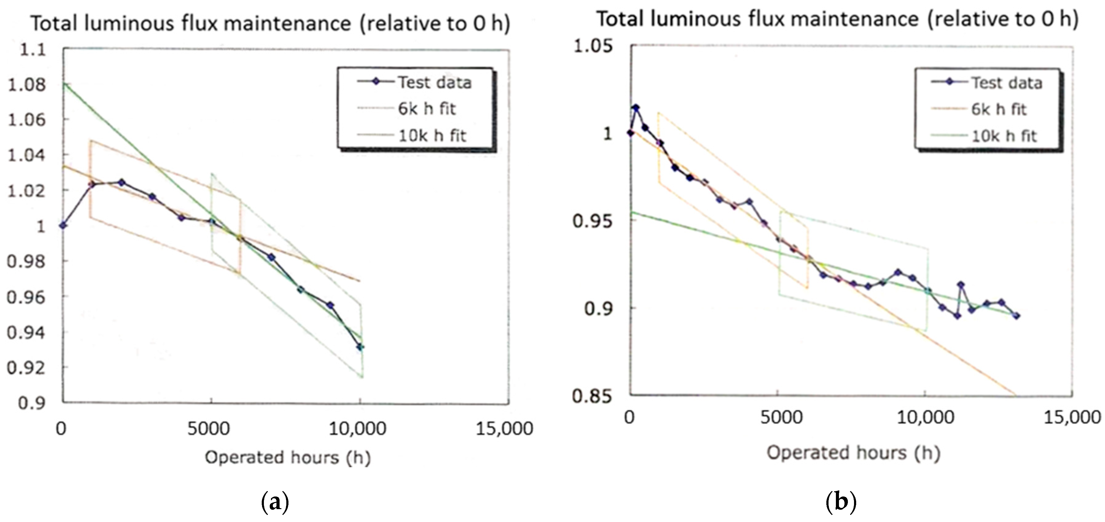
Figure 2.
Theoretical pn-junction temperature increase during an LM-80 test in case of (a) a high-power and (b) a mid-power LED, as the function of the forward current, the thermal resistance, the zero-hour radiant efficiency and the reached luminous flux decay (assuming a constant thermal resistance and a Figure 3. V forward voltage). Note that the curves on (a) and (b) are identical implying that the junction temperature increase may affect high- and mid-power LEDs equally, depending on the thermal resistance.
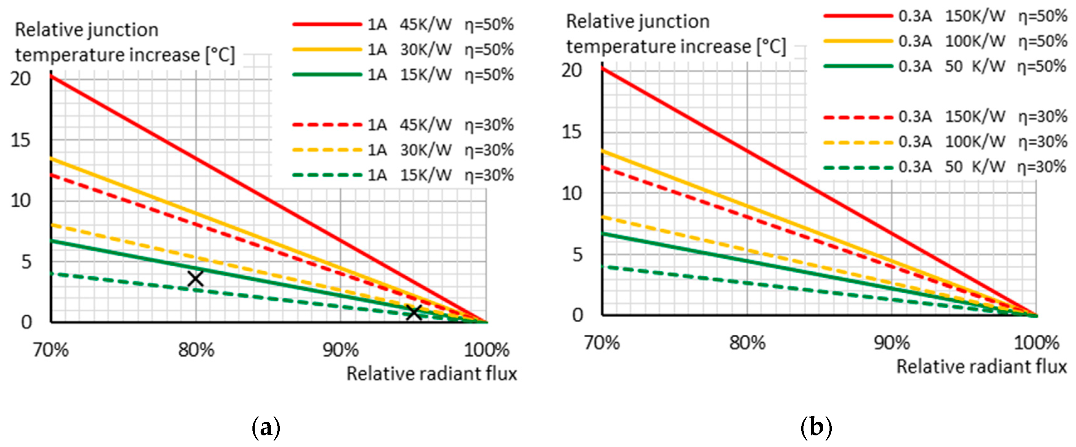
Figure 3.
Effects of the increase in the forward voltage and in the thermal resistance on the pn-junction temperature increase during an LM-80 test. The initial parameters are: 1 A forward current, 40% radiant efficiency, 15 K/W thermal resistance, 3 V forward voltage. The figures show the junction temperature increase during the test as the function of the end of test thermal resistance and forward voltage. The end of test relative light outputs are (a) 95% and (b) 80%. The black crosses indicate values corresponding to that of in Figure 2a.
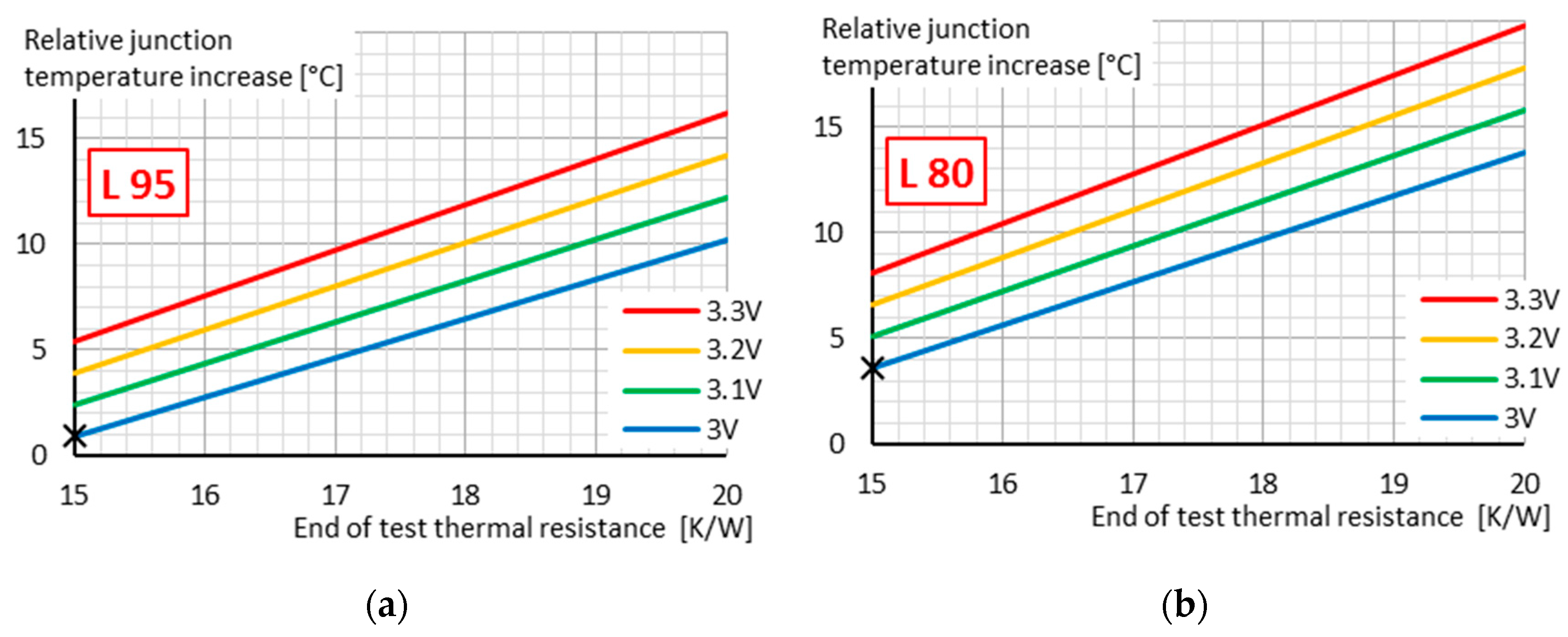
Figure 4.
Shift of the forward voltage—forward current characteristics during the first 9000 h of a Luxeon Z LED sample (aged at 85 °C case temperature and 1 A forward current).
Figure 4.
Shift of the forward voltage—forward current characteristics during the first 9000 h of a Luxeon Z LED sample (aged at 85 °C case temperature and 1 A forward current).
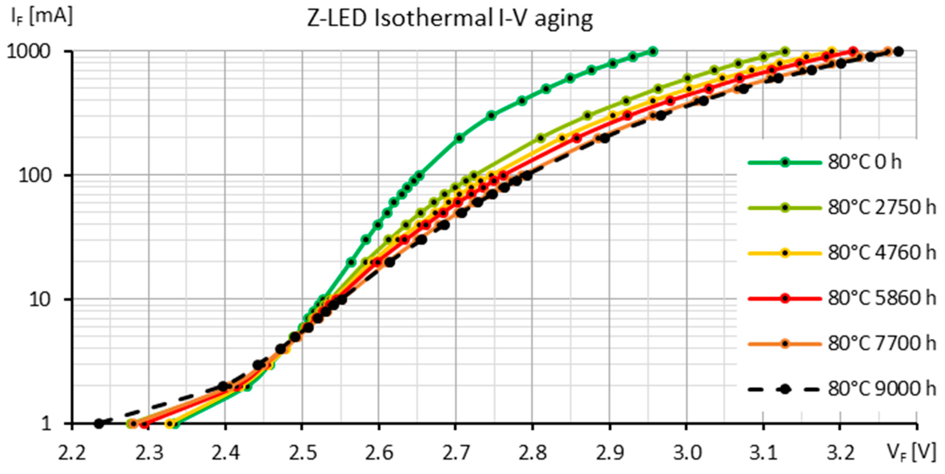
Figure 5.
Pn-junction temperatures of the tested mid-power LED (#S11) over the testing time, measured at 300 mA forward current, (a) at 25 °C and (b) at 55 °C ambient temperatures.
Figure 5.
Pn-junction temperatures of the tested mid-power LED (#S11) over the testing time, measured at 300 mA forward current, (a) at 25 °C and (b) at 55 °C ambient temperatures.

Figure 6.
Measurement and simulation results of the aged mid-power blue LED; the logarithmic regression fitting parameters to the 85 °C values are indicated just as an example.
Figure 6.
Measurement and simulation results of the aged mid-power blue LED; the logarithmic regression fitting parameters to the 85 °C values are indicated just as an example.
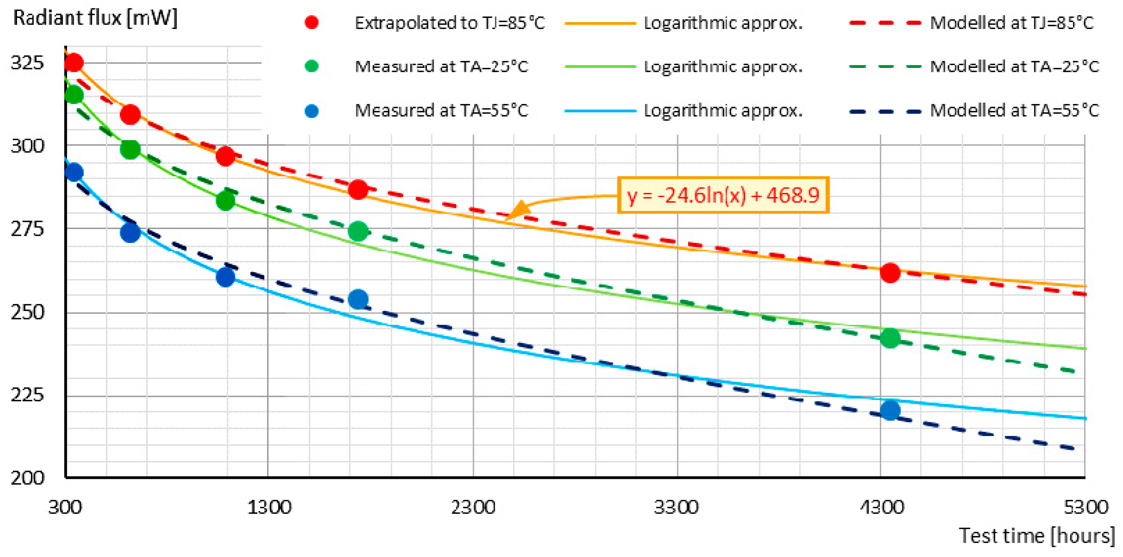
Figure 7.
(a) Averaged LM-80 measurement results of 9 pieces of Luxeon Z samples and extrapolation until 50k hours ( = 120 °C, = 1 A); (b) Exponential curve fit to the LM-80 measurement set along with the eight assumed aging trends.
Figure 7.
(a) Averaged LM-80 measurement results of 9 pieces of Luxeon Z samples and extrapolation until 50k hours ( = 120 °C, = 1 A); (b) Exponential curve fit to the LM-80 measurement set along with the eight assumed aging trends.
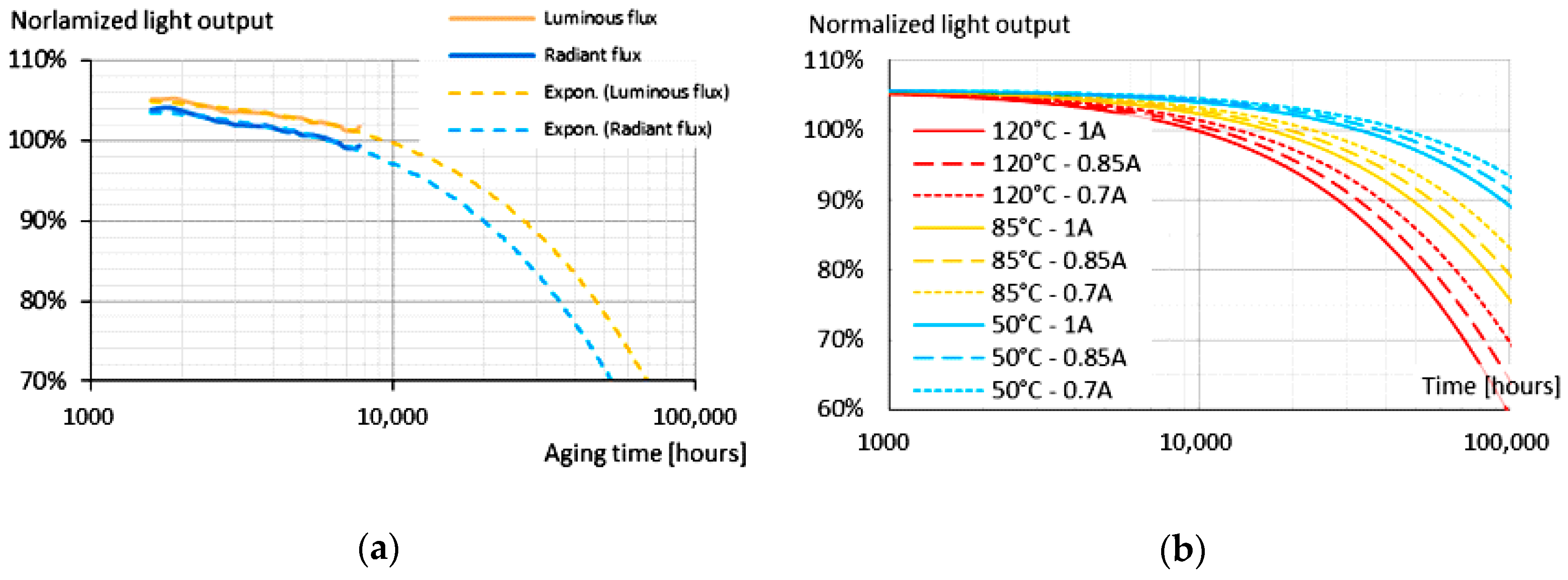
Figure 8.
Illustration of the aging model; the simulation conditions are changed after 30,000 h.
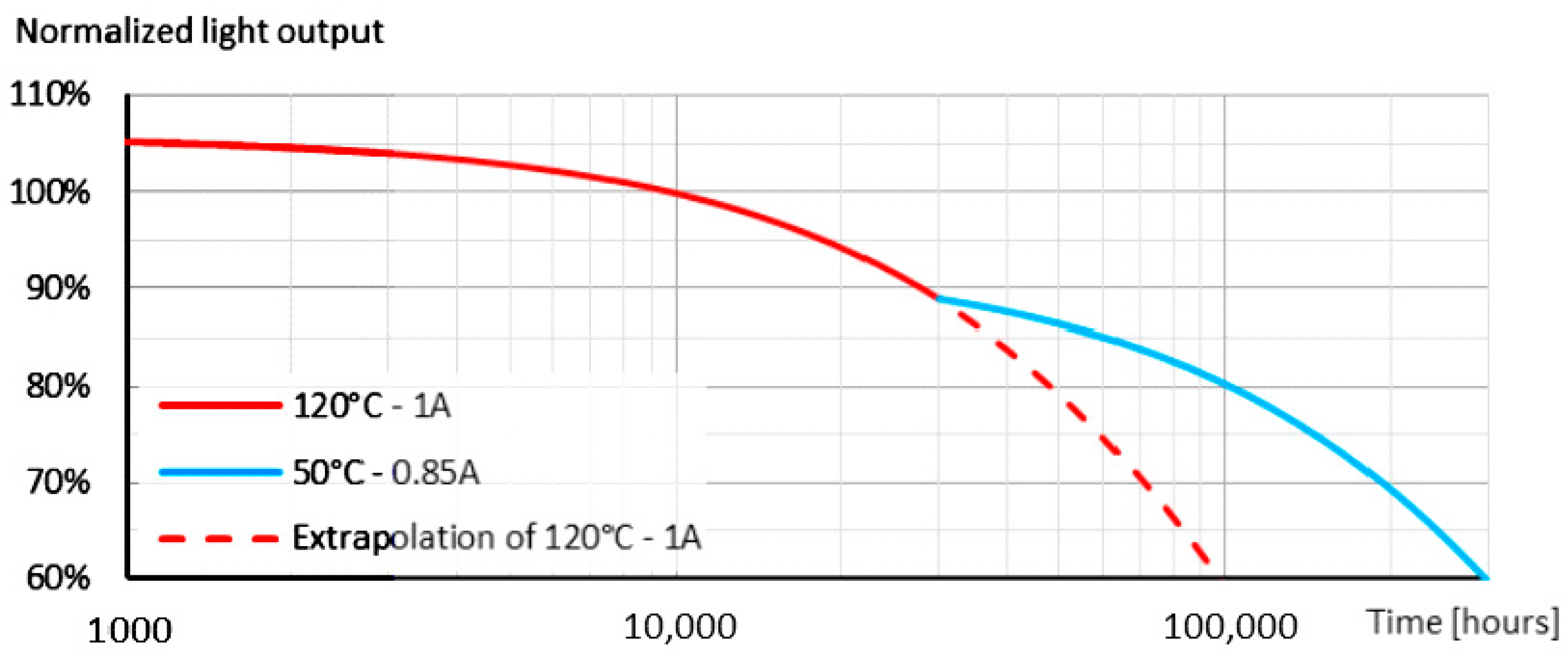
Figure 9.
The forward currents applied during the simulation (the absolute maximum DC forward current of the Luxeon Z LEDs is 1 A).
Figure 9.
The forward currents applied during the simulation (the absolute maximum DC forward current of the Luxeon Z LEDs is 1 A).
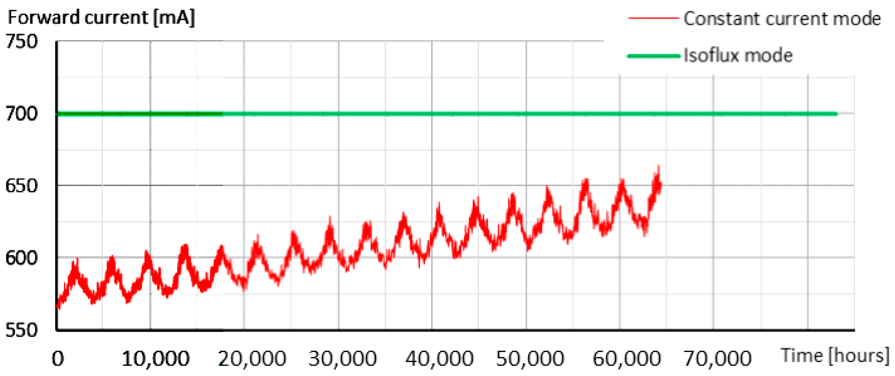
Figure 10.
Simulated light output of a Luxeon Z LED.
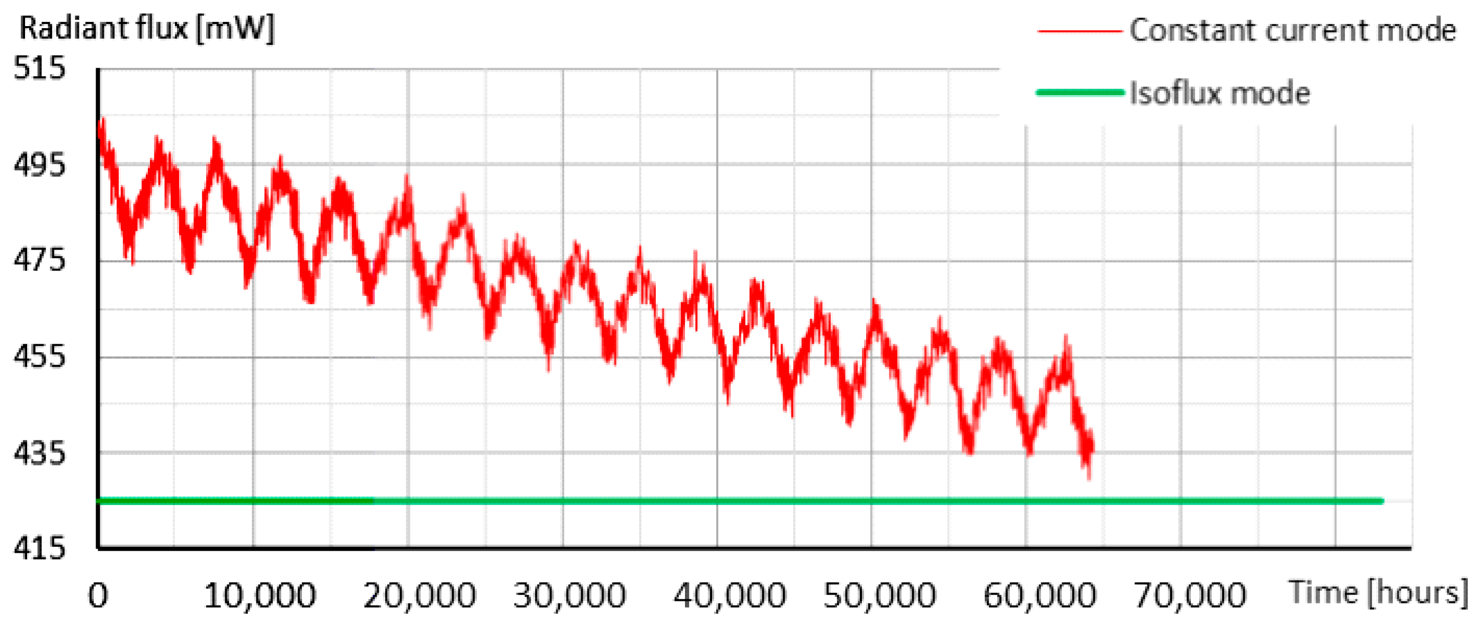
Figure 11.
Simulated lifetime budget of a Luxeon Z LED.
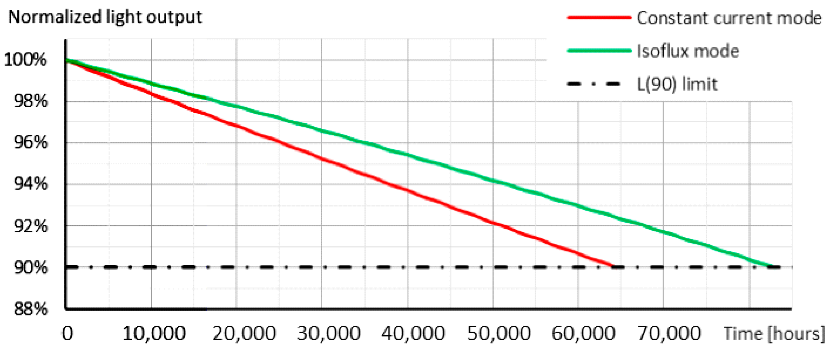
Figure 12.
(a) Total luminous and radiant flux maintenance curves with their extrapolation [73]; (b) Time dependence of the model parameters: change of the saturation currents [73].
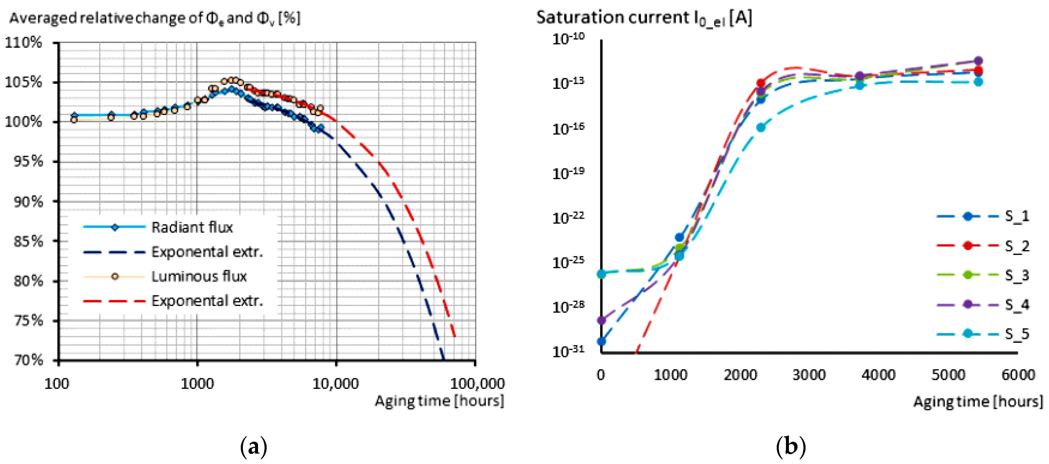
Figure 13.
The sample mid-power LEDs mounted on FR4 strips; the printed circuit boards were provided with increased thermal interfaces for better cooling capabilities.
Figure 13.
The sample mid-power LEDs mounted on FR4 strips; the printed circuit boards were provided with increased thermal interfaces for better cooling capabilities.
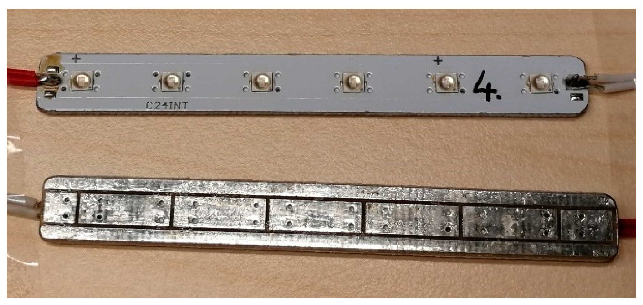
Figure 14.
(a) A failed and (b) an unburnt sample of the investigated mid-power LEDs.
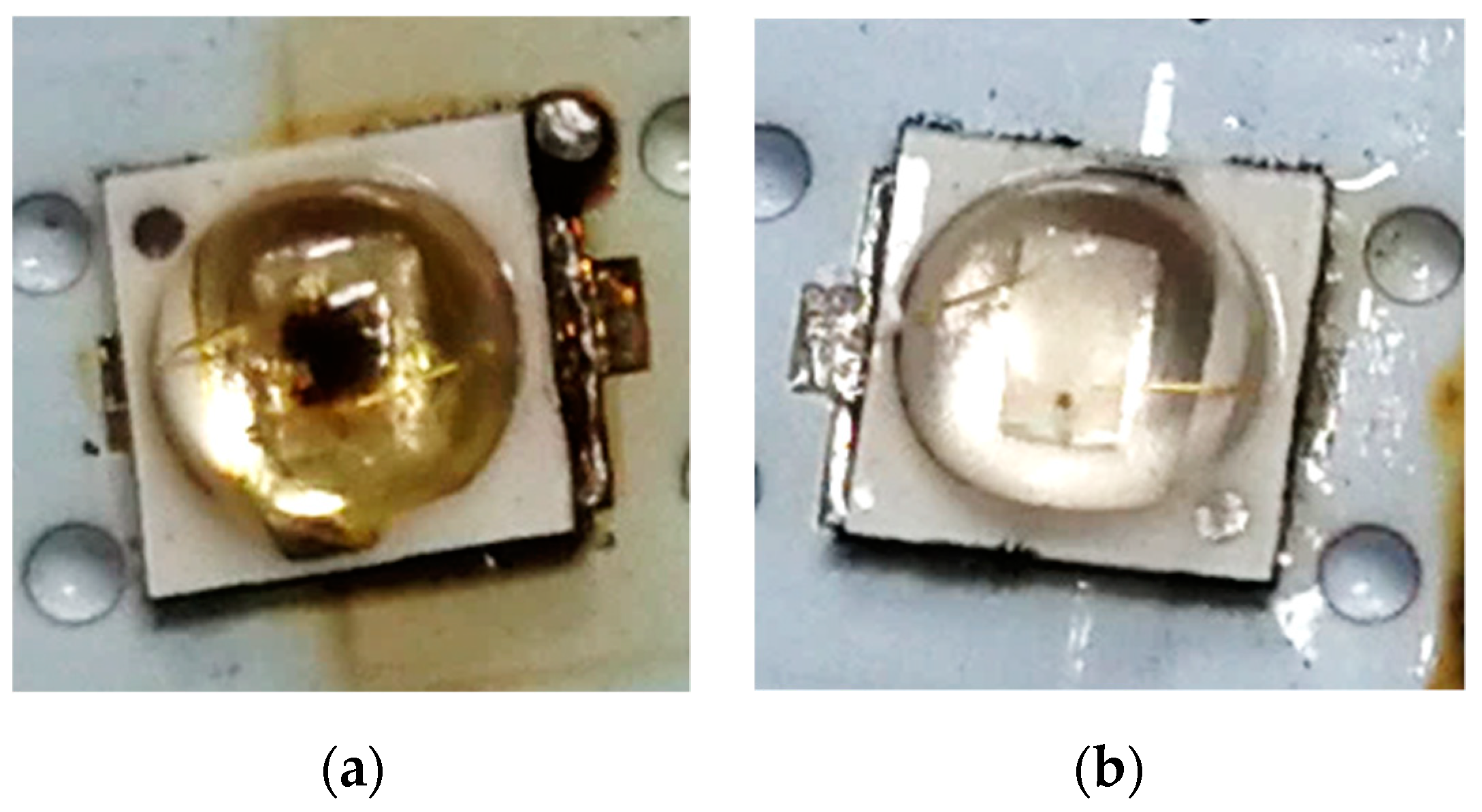
Figure 15.
The attained total radiant flux maintenance results of the mid-power blue LEDs, sorted by case temperature and forward current.
Figure 15.
The attained total radiant flux maintenance results of the mid-power blue LEDs, sorted by case temperature and forward current.
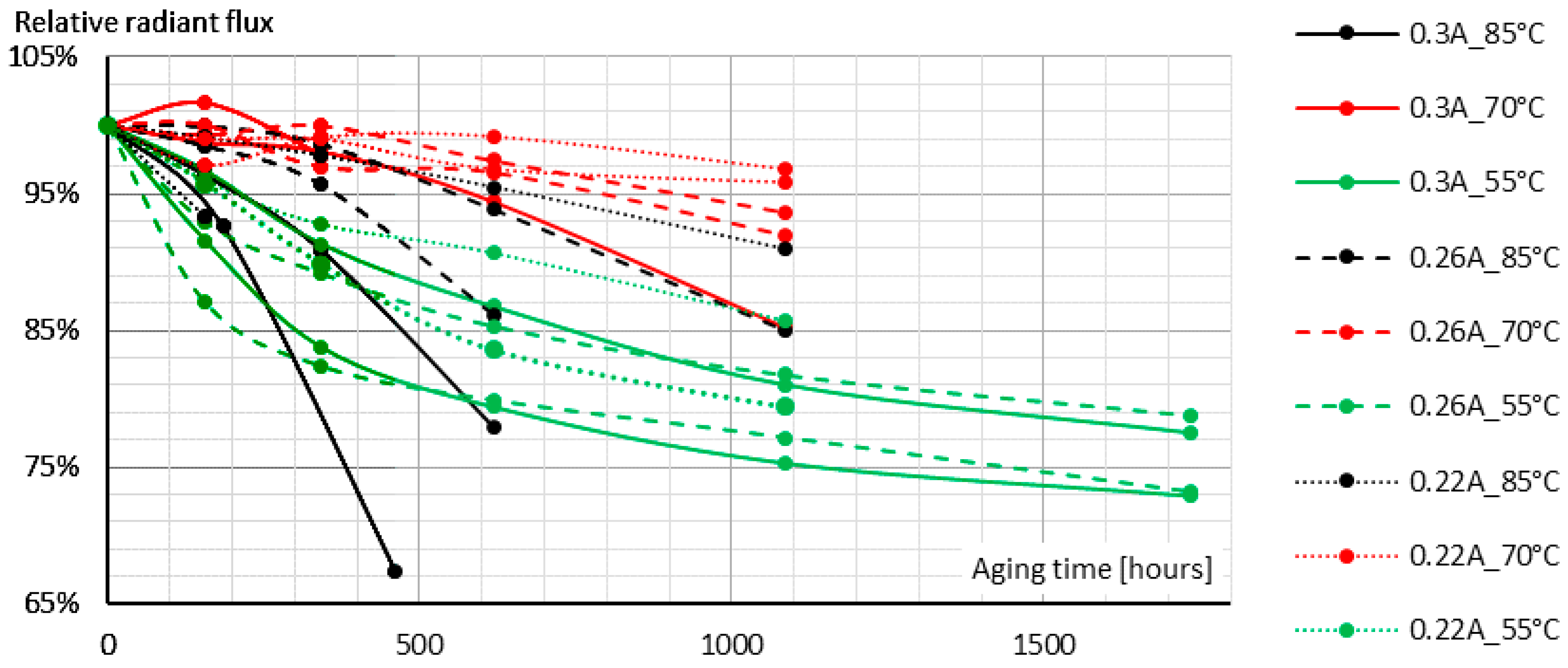
Figure 16.
Electrical (a–c) and optical (d–f) model parameters of #S07.
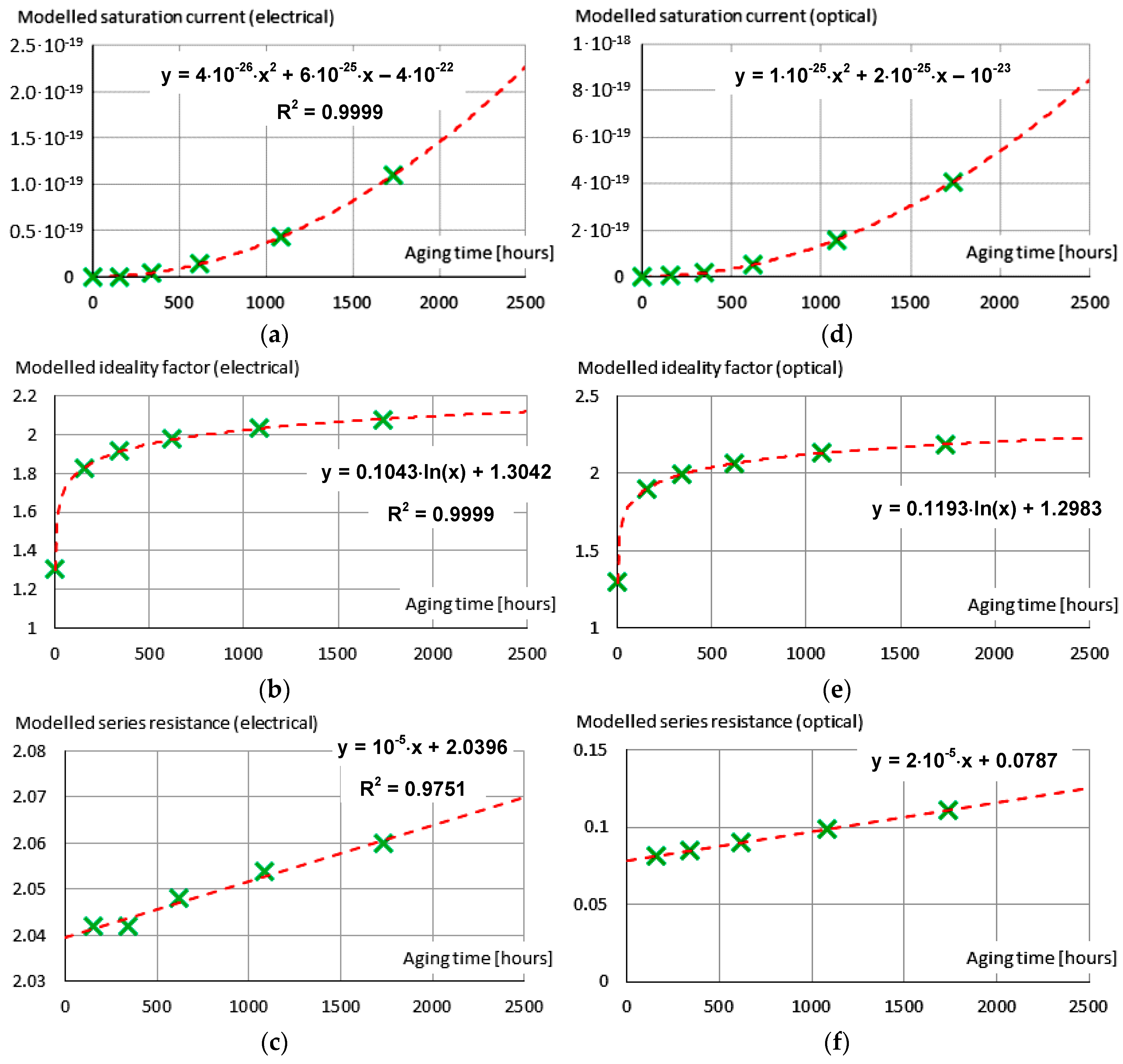
Figure 17.
(a) Comparison of the simulated and measured total radiant flux maintenance curves of #S07; (b) The simulation results of #S07 with higher time resolution—the discontinuity can be clearly seen.
Figure 17.
(a) Comparison of the simulated and measured total radiant flux maintenance curves of #S07; (b) The simulation results of #S07 with higher time resolution—the discontinuity can be clearly seen.
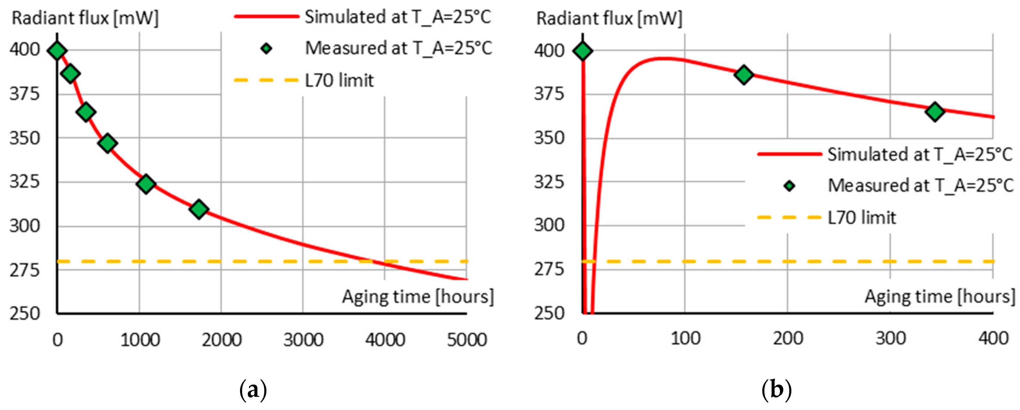
Figure 18.
Simulated and measured total radiant flux maintenance of #S07 (a) and sample #S11 (c); Measured and simulated time function of the forward voltage of sample #S07 (b) and sample #S11 (d).
Figure 18.
Simulated and measured total radiant flux maintenance of #S07 (a) and sample #S11 (c); Measured and simulated time function of the forward voltage of sample #S07 (b) and sample #S11 (d).
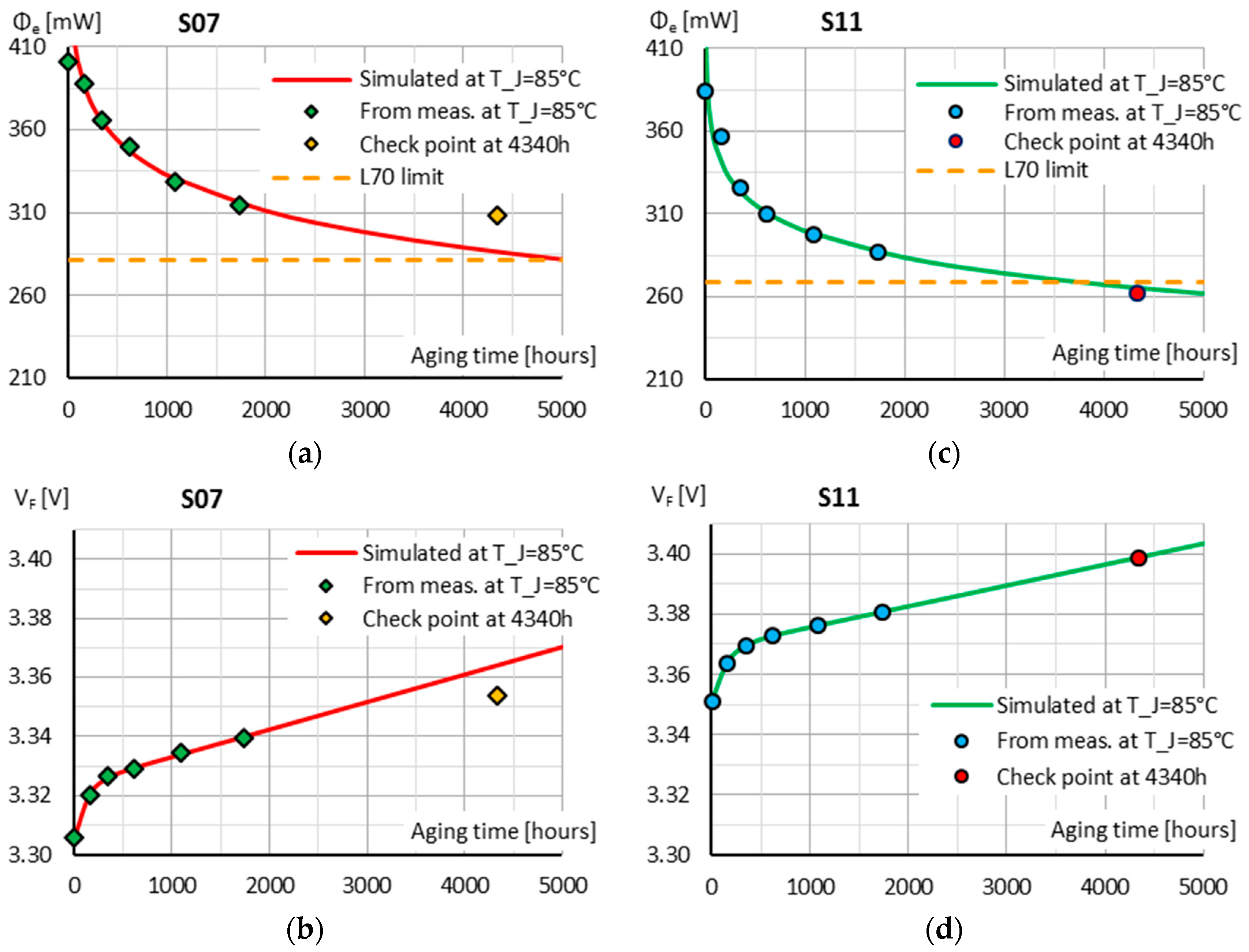

Table 1.
Aging models of different decay rates with the closed form solution, i.e., the integral form (after [49]).
Table 1.
Aging models of different decay rates with the closed form solution, i.e., the integral form (after [49]).
| # | Decay Rate | Integral Form | |
|---|---|---|---|
| 1 | |||
| 2 | |||
| 3 | Model 1 + Model 2 | ||
| 4 | |||
| 5 | Model 1 + Model 4 | ||
| 6 | |||
| 7 | |||
| 8 | Model 2 + Model 7 | ||
| 9 |
Table 2.
Elapsed time till 50k hours of operation of a streetlighting luminaire in years, in Hungary.
Table 2.
Elapsed time till 50k hours of operation of a streetlighting luminaire in years, in Hungary.
| Dark-Hours in-Between | 50k Dark-Hours (Years) | Dark-Hours during a Year (Hours) | |
|---|---|---|---|
| Sunset to Sunrise | 12 years | 4291 h | |
| Civil | Twilights | 13 years | 3875 h |
| Nautical | 15 years | 3373 h | |
| Astronomical | 18 years | 2802 h | |
Table 3.
Comparison of operation with constant forward current (700 mA) and with constant light output (425 mW), simulated with the help of our LED aging theory.
Table 3.
Comparison of operation with constant forward current (700 mA) and with constant light output (425 mW), simulated with the help of our LED aging theory.
| Examined Parameter | Advantages of the Proposed CLO | ||
|---|---|---|---|
| Time to L(90) (hours) | 64.4k h | 83k h | +29% |
| Working years till L(90) | 16.7 years | 21.4 years | +4.7 years |
| Electricity consumed till 64.4k hours | 130.8 kWh | 112.8 kWh | −13.7% |
| Used energy in the 1st operational year | 7.9 kWh | 6.5 kWh | −17.7% |
Table 4.
The error made by the model compared to the measurement results at 4340 h.
| Sample | Mismatch (mV) | Mismatch Compared to the Zero-Hour Results (%) | Mismatch (mW) | Mismatch Compared to the Zero-Hour Results (%) |
|---|---|---|---|---|
| #S07 | 10.2 mV | 0.3% | −21.7 mW | 5.4% |
| #S11 | 0.1 mV | 0.003% | 3.2 mW | 0.8% |
© 2020 by the authors. Licensee MDPI, Basel, Switzerland. This article is an open access article distributed under the terms and conditions of the Creative Commons Attribution (CC BY) license (http://creativecommons.org/licenses/by/4.0/).
Share and Cite
MDPI and ACS Style
Hegedüs, J.; Hantos, G.; Poppe, A. Lifetime Modelling Issues of Power Light Emitting Diodes. Energies 2020, 13, 3370. https://doi.org/10.3390/en13133370
AMA Style
Hegedüs J, Hantos G, Poppe A. Lifetime Modelling Issues of Power Light Emitting Diodes. Energies. 2020; 13(13):3370. https://doi.org/10.3390/en13133370
Chicago/Turabian StyleHegedüs, János, Gusztáv Hantos, and András Poppe. 2020. "Lifetime Modelling Issues of Power Light Emitting Diodes" Energies 13, no. 13: 3370. https://doi.org/10.3390/en13133370
Note that from the first issue of 2016, this journal uses article numbers instead of page numbers. See further details here.