1. Introduction
The increasing need for electricity and the risks of environmental pollution and global warming are the main problems increasing the interest in renewable and clean energy sources [
1]. Solar energy sources using photovoltaic (PV) modules recently have the main focus among other renewable sources. This is due to several reasons such as the abundance of the solar irradiance, the photovoltaic (PV) phenomenon, by which a direct conversion is achieved from solar radiation to electricity, employable at both small and large scale, non-polluting, clean and reliable energy sources. The increase in the temperature of the silicon-based technology PV modules has direct effect on the current–voltage (I–V) characteristics of the device, that is, adversely affecting the power production and causes a significant drop in efficiency [
2,
3]. Therefore, it is insufficient to rely only on the rated efficiency to estimate the output power. One has to consider the operating temperature of the PV module as well as other environmental conditions and structural parameters [
4]. The temperature of the PV module is affected by the module material compositions, mounting structure and the environmental conditions [
5,
6]. Multiple heat sources are physically contributing to the increment of the module temperature [
5]. The first is the incoming short-wave solar irradiance, where only up to 20% will be converted to electrical energy, and the rest will be converted to thermal energy [
4,
7]. The second heat source is the long-wave infrared radiation. Accurate temperature prediction is not only needed for a precise prediction of the output power, but is also essential for estimating lifetime and quantifying the degradation of PV modules [
7,
8,
9,
10].
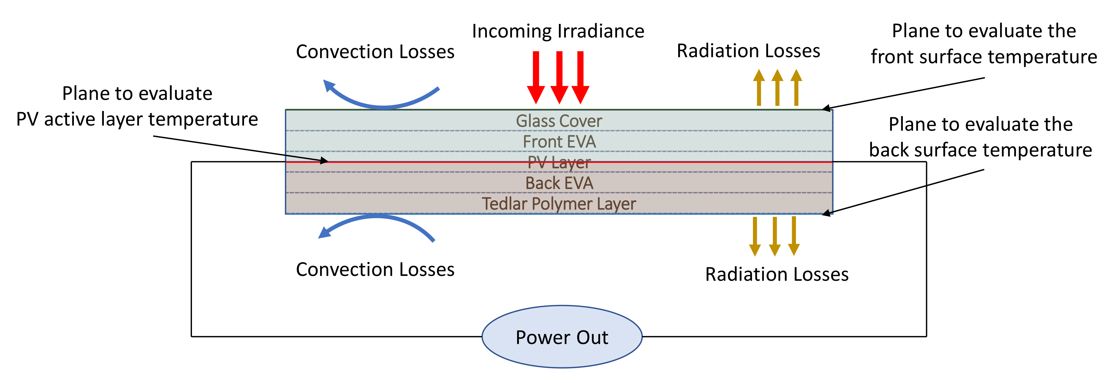
The heat generated in the PV module is conducted through the stacked layers of the PV module to the external surfaces (front and back surface). Radiation, forced convection and free convection heat transfer mechanisms are involved in dissipating the generated thermal energy from the surfaces to the surrounding environment. Therefore, a robust PV thermal modelling is required to estimate the operating temperature of the PV module under the given environmental, physical and structural conditions. These conditions are represented by physical parameters, which act as an input for the model.
The main objective of this work is to propose a novel thermal model to estimate the PV module temperatures at three different planes: The semiconductor p-n junction (electronic junction temperature), the front and the back surface of the PV module. The proposed model is constructed by new combination of effective sub-models found in the literature and including a novel solution for considering the effect of the module tilt angle on the forced convection heat transfer mechanism.
5. Detailed Construction of Thermal Model
Constructing the thermal model in this research work is based on the approach of treating the PV module as a single block of material and employing the HBE, including different heat transfer mechanisms.
Figure 2 shows the thermal behaviour of a PV module that described by the HBE.
The model will provide the PV module junction temperature as well as the temperature difference to both surfaces. Therefore, both front and back surface temperatures will be estimated. This result will be useful in the validation phase because then we can compare the back surface estimated temperature to the measured one by a thermometer attached to the backside of the PV module. The model was constructed based on different, already existing models from the literature (see
Section 4). However, the new model was constructed by incorporating sub-models of different existing models in a new and unique way to yield a new model with improved accuracy. For this, different sub-models of the above described models were combined and tested, and the combination with the best accuracy was chosen as the mode for this paper. The total absorbed energy is consisting of two components and given as
where
is the rate of thermal energy absorbed by the tempered glass layer,
is the energy absorbed by the semiconductor layer,
is the transmittance of the glass layer,
and
is the absorptivity of the front glass and semiconductor layers, respectively.
In this paper, we consider a static model, that is, we assume that the module output power predicted by the proposed model is required only with a time resolution that enables the the temperature to reach a steady state. Therefore, the HBE component which is related to the material thermal capacity is neglected and the converted energy is limited only to the electrical produced component, which is given as
The radiation heat losses trough both front and back surfaces are calculated using the following expressions, respectively [
8].
The view factors are calculated using the expressions given in
Section 4.3.3 (point number 10). The sky temperature is,
for clear sky condition where
for overcast condition [
29]. The ground temperature is assumed to be equal to the ambient temperature.
Both free and forced convection mechanisms are considered in creating this thermal model. Their overall effect is calculated by combining their effect using Equation T 1.2 from
Table 1. For both mechanisms, we treat the front and back surface individually because the properties of the film layer at the boundary of each one are different. The free convection heat loss is determined using Equations (
14) to (
18), in which the subscript
x refers to the front (
f) or back (
b) surface; therefore, during implementation, the equation has to be rewritten for each surface.
For estimating the forced convection coefficients (for both surfaces), we modify the expressions used by Kayhan [
13], given as
The introduced modification can be seen in Equation (
20) where we added a novel coefficient (
H), which is defined as the forced convection adjustment coefficient for both front and back surfaces. This coefficient modulates the relationship between the tilt angle and the wind effect on the amount of heat loss by forced convection. This coefficient is calculated as
where
m is an empirical factor estimated with the help of measurement data. The following points explain the fundamental concept behind the coefficient
H by considering PV module mounted with different tilt angles and assuming that the value of
m is equal to 2.
0 tilt angle:
- -
The front surface will undergo a maximum effect of the wind that will sweep the hot air away. This fact is ensured by Equation (
21), which will be evaluated to 1. That is, the expression used for calculating the heat loss by forced convection will not be disturbed by the tilt angle.
- -
For a typical PV system, there are two facts: First, the system is consisting of many PV modules with a defined density. Second, PV modules are mounted close to the ground in case of flat and small tilt angles. Therefore, the wind will have no considerable effect on the back surface of the PV module. Equation (
22) will be evaluated to zero for a flat surface; that is, the forced convection heat loss from the back surface will be neglected in this case.
60 tilt angle:
- -
This implies that the wind will face resistance from the front surface of the PV module compared to the case of flat mounting. Therefore, reducing the ability to sweep out the hot air away from the surface. Equation (
21) will be evaluated to
. That is, the tilt angle will be a reason for reducing the amount of heat loss by forced convection.
- -
The lower surface will be facing the wind, which was not the case for a flat-mounted module. Equation (
22) will be evaluated to
. Thus, heat loss by forced convection is much higher compared to flat or small tilt angles. However, it is still lower compared to the front surface.
90
tilt angle: Both front and back surfaces will be directly facing the air flow. Therefore, neglecting the wind direction for its minor effect compared to its speed [
25,
26], the wind will equally act on both surfaces. Both Equations (
21) and (
22) will be evaluated to
.
Therefore, we consider that the PV module tilt angle will control the amount of heat losses from both surfaced. For tilt angles between 0 and 90, the front surface heat loss by forced convection is higher compared to the back surface. Increasing the tilt angle (within this range) produces lower forced convection heat loss from the front surface and higher from the back surface.
We claim that m is a factor that affects the relationship between the tilt angle and the heat loss by forced convection by involving other installation parameters. These parameters include the PV modules installation density, the elevation from the ground and the thickness at the module edges at which the wind speed drops to zero. From experience, we found that this empirical factor has a value in the range between 1.5 and 2. Therefore, in this paper, we consider scanning this range with a specific resolution and running the model for each value. By increasing the resolution more, the value of m can be determined more accurately. Based on experience, We consider as a resolution value considering a trade-off between the computational cost and accuracy. Therefore, we consider running the thermal model six times after which we decide what is the best value for m (by monitoring the error indication parameters) to be fixed for the module under investigation.
Once we have the value of the empirical factor
m, we substitute it in Equations (
21) and (
22) to determine the forced convection adjustment coefficient for the front and back surface, respectively. For each surface, the overall convection coefficient and the corresponding rate of convection thermal energy losses can be calculated using the Equations T 1.2 from
Table 1 and
6.
The proposed model also considers the following points.
The characteristics length is considered as the longest dimension of the PV module.
The model operates to determine the PV electronic junction temperature. This temperature is correlated to the front and back surfaces employing temperature differences. Each temperature difference is defined as the total heat losses from the corresponding surface multiplied by the thermal resistivity of half of the PV structure (the volume between the half of the semiconductor layer plane and the corresponding surface plane), as shown in
Figure 2.
The Newton–Raphson iterative method is employed to solve the model and calculate the output PV layer, front surface and back surface temperatures.
Therefore, with each iteration, the following two equations are evaluated to calculate the front and back surface temperatures, respectively,
where
and
are the total thermal losses from the front and back side of the PV module, respectively.
, and
are the thermal resistivity of the PV module, between the front and back surfaces and the active layer, respectively.
6. Results and Discussion
This model has been validated using a polycrystalline and an amorphous PV module. The validation data of the polycrystalline module has been taken from a reference [
9]. Our measurement system has been used to collect the amorphous module validation data. This measurement system provides data such as PV module back surface temperature, full I–V curve, global solar irradiance, ambient temperature and wind speed. The global irradiance was measured by Delta Ohm LP RAD 03 piranometer that detect solar irradiance ranging from 0 to 2000 W/m
. The temperature of the PV module is recorded using a circuit board attached to the back side of the module with a thermal conductive adhesive. The circuit includes a temperature sensor IC (MAX6603ATB+T). The accuracy of the circuit is ±0.8
C at +25
C. The ambient temperature is measured using PT100 resistance thermometers. Wind speed data is taken from a wind turbine FD2.5-300 which is capable of measuring range of 0 to 60 m/s with an accuracy of ±0.3 m/s.
Table 6 shows the technical specifications and physical parameters of both modules, which are required for running the model.
To verify the model, we use measurement data including irradiances, ambient temperatures and wind speed that have been recorded for two different full days for each module. For the amorphous module, the two days were the 5th and the 11th of October. For the polycrystalline module, the two days were the 3rd and the 26th of July. The main difference between the two days of each module is the wind speed. The average wind speed is
m/s on the 26th and
m/s on the 3rd of July, while it is
m/s on the 5th and
m/s on the 11th of October. As mentioned in
Table 6, each module has a different tilt angle. Based on our experience, we claim that the module tilt angle has a significant effect on the value of the thermal energy losses by forced convection. As described in the model introduced in
Section 5, we introduced a forced convection adjustment coefficient (
H) and its empirical factor (
m). In this regard, we report that the value of
m typically takes a value between 1.5 and 2. We calculate this factor by scanning its range and running the model with a step of
.
For evaluating the proposed model and validating the results we use two error indication parameters: one is the root mean square error (
) and the other is the correlation coefficient (
r). These parameters are used, as shown in
Table 7, to compare the module’s back surface temperature for each day (entire day measurement) of the two modules with the estimated values using the proposed model for different values of
m.
Based on the results shown in
Table 7, we chose a value of
for the polycrystalline module and
for the amorphous module to be used in this study, as these values give the best results.
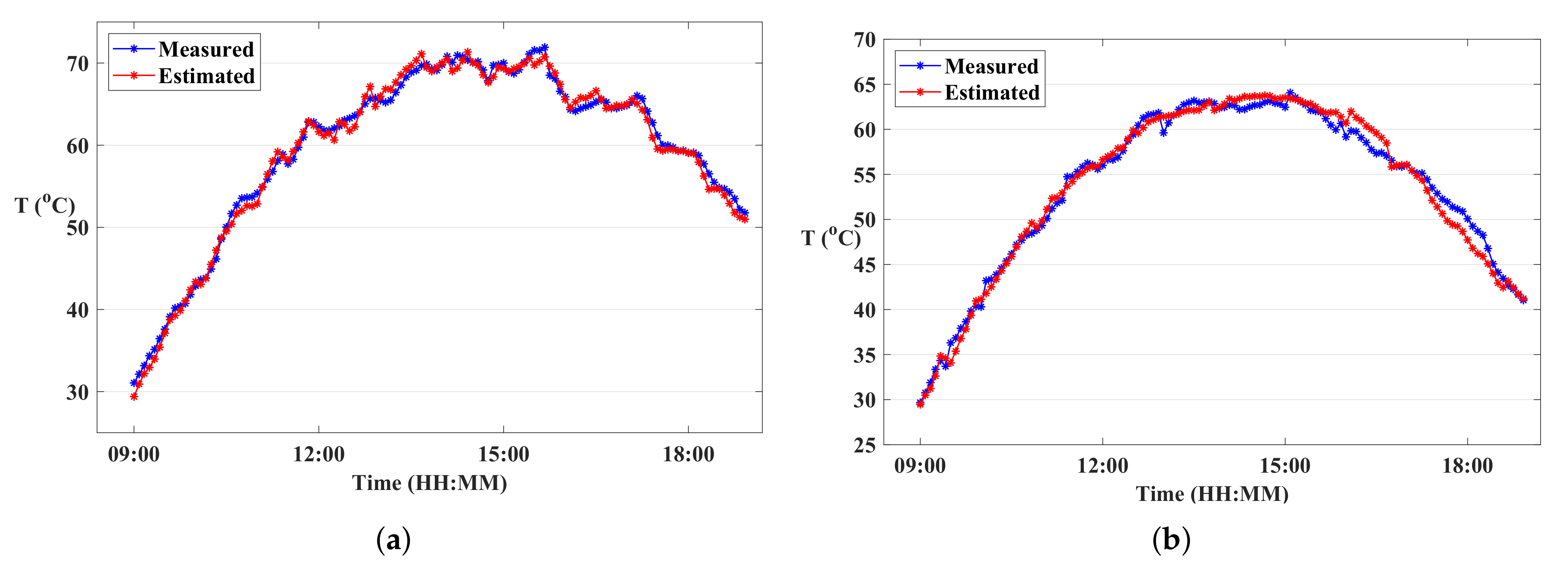
Figure 3 shows both the measured and the estimated PV module back surface temperature for the polycrystalline module, for the two investigated days: 3rd and 26th of July. Each curve includes 120 points as a result of recording the temperatures every 5 min between 9 am and 7 pm.
Figure 4 shows both the measured and the estimated PV module back surface temperature for the amorphous module, for the two investigated days, 5th of October (49 points between 9 am and 1 pm) and 11th of October (71 points between 9 am and 3 pm).
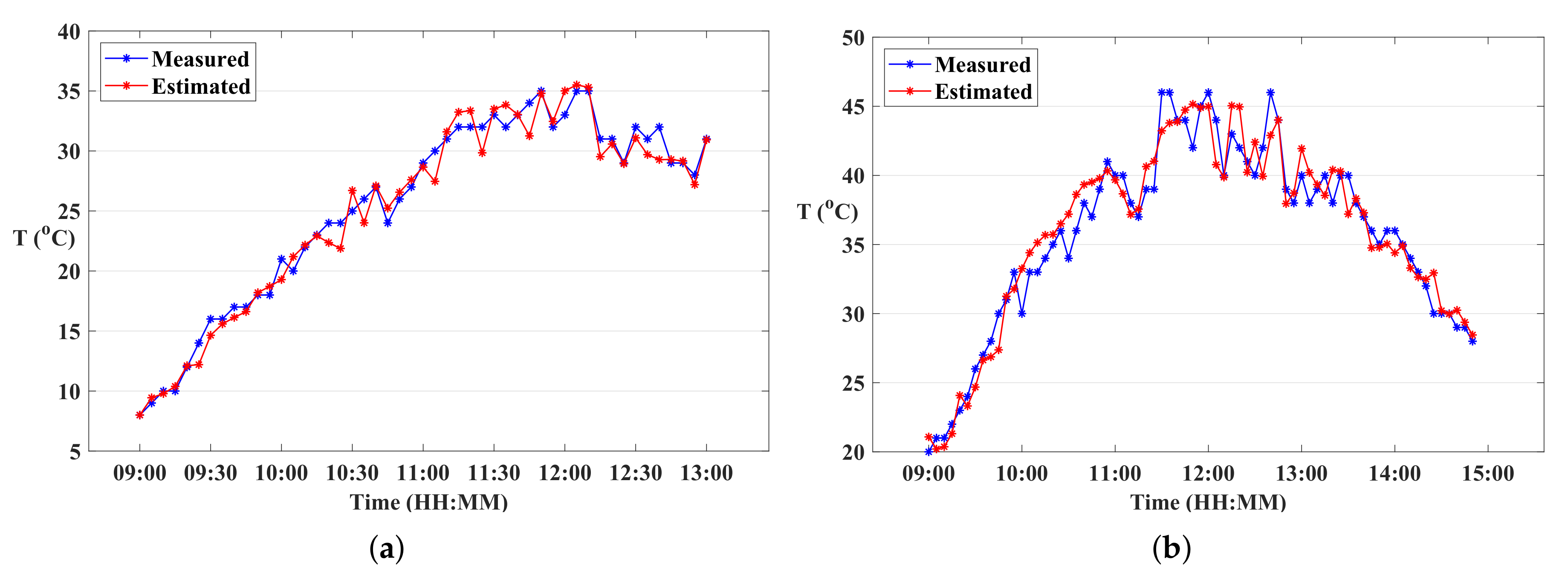
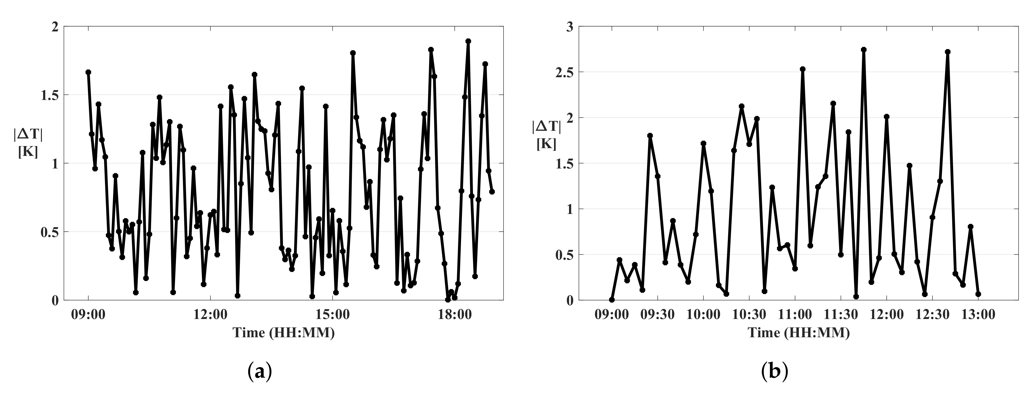
Figure 5 shows the absolute value of the temperature difference between the measured and estimated values of the back surface temperature using the proposed model for both modules.
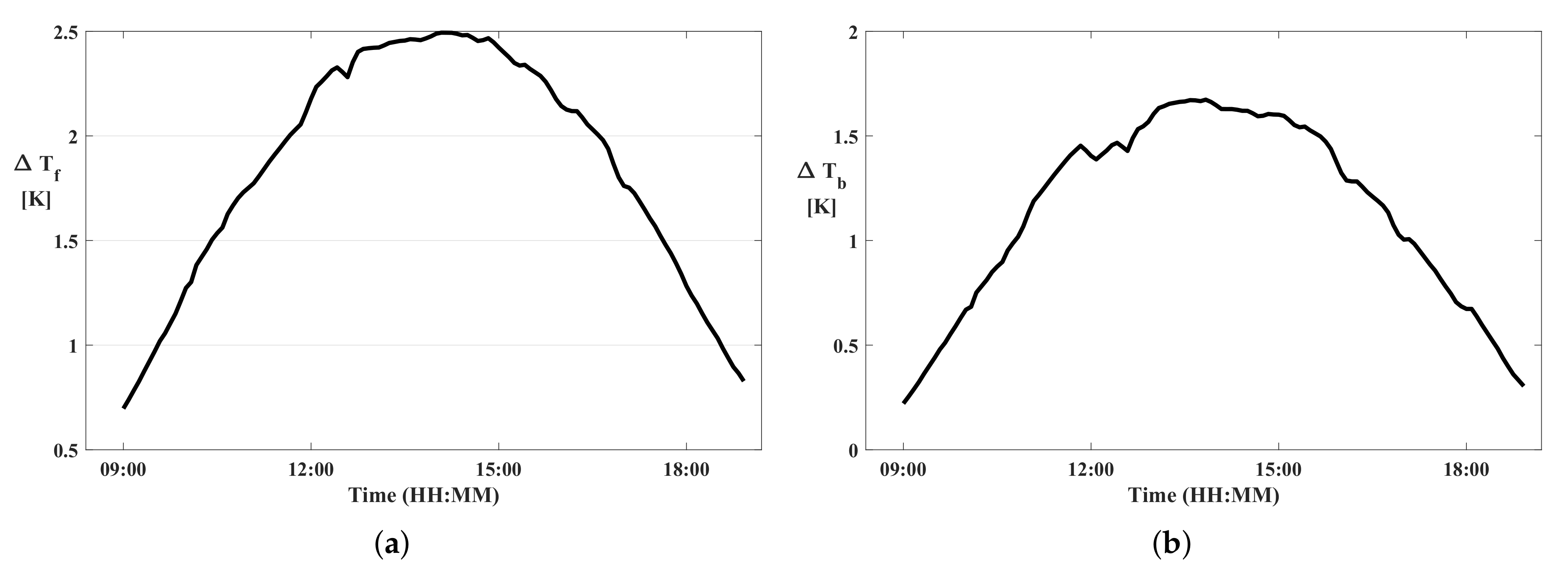
Figure 6 shows the relationship between the junction temperature and both surfaces temperatures. It illustrates how these temperature differences are changing with the time of day. Therefore, it will provide a clear picture of the temperature profile across the PV module. The temperature difference to the front surface (
) is ranging from
to
, with an average value of 1.86
C. The temperature difference to the back surface is between
and
with 0.96
C as an average value.
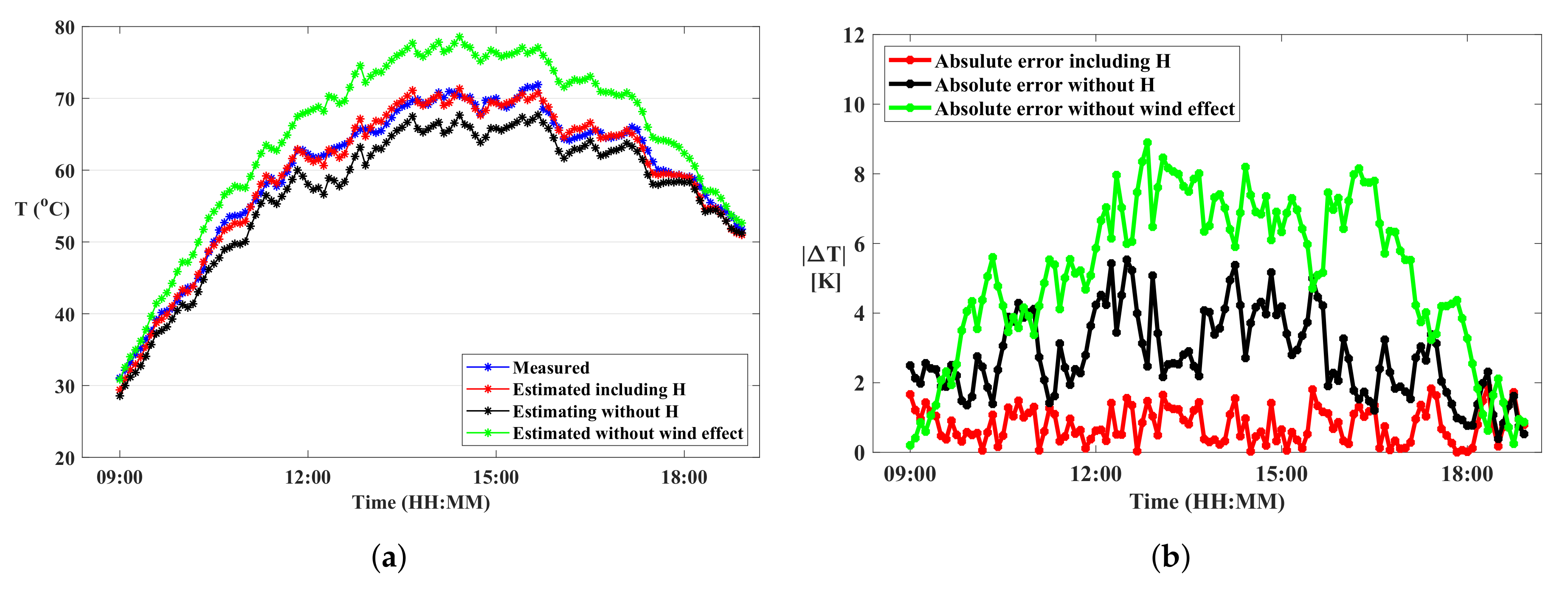
Figure 7 highlight the importance of the novel coefficient and the consideration of the tilt angle in the forced convection, introduced in this paper. The same figure also shows the effect of neglecting the wind in the thermal model.
Figure 7a compares the measured back surface temperature (blue colour) to the estimated temperature with the coefficient
H (red colour), without the coefficient
H (black colour), and without wind effect (green colour), for the polycrystalline module (measurements used for 3rd July).
Figure 7b shows the absolute error to compare different situations.
According to the results shown above, we summarise the discussion with the following points.
One of the focus points of the proposed model is the special dependence of forced convection mechanism on the module tilt angle.
Two modules made with different technologies and mounted with different tilt angles were used to validate the proposed model. A forced convection adjustment coefficient (H) has been considered for this purpose, which includes an empirical factor (m). We calculate this factor by scanning its range as discussed above.
For each module, the model has been validated using measurements of two days with different average wind speeds.
Table 7 shows the proposed model’s ability to estimate the temperature with high accuracy characterised by the two error quantifying parameters, namely,
and
r. It is worth mentioning that the model provides low error rate for all values of
m. However, the highest accuracy is realised at an optimum value of the factor
m.
From
Figure 3 and
Figure 4, we see that the model results represented by the backside estimated temperature followed the experimentally measured values for PV modules of different technologies, different tilt angles and different wind speeds by measurements collected on two different days for each module.
Figure 5 shows the absolute difference between the measured and the estimated values using the proposed model for both modules.
Figure 5a shows that this value is always below 2
C, with an average value of
C for the polycrystalline module (measurements used for 3rd July).
Figure 5b shows similar results for the amorphous module.
Figure 7b shows the substitutional effect of the coefficient
H on the thermal model, enabling accurate temperature estimation for the PV modules. The same figure also shows that large error is produced in case of neglecting the wind effect (neglecting the forced convection heat transfer mechanism).
Figure 6 shows that the temperature difference between the PV electronic junction plane and both surfaces reach their maximum values around the midday time at which both ambient and electronic junction temperature are at their maximum values. This happens because the ambient temperature is higher at midday; thus, the temperature difference between the module surface and the ambient is smaller that will reduce the rate of the heat loss from the module to the surrounding.
Table 8 shows the achieved accuracy of the proposed model using the two modules under different environmental conditions, represented by two introduced error quantifying parameters
and
r.
For the same module, typically, > . Therefore, the top surface temperature is slightly lower than the backside temperature due to, relatively, more effective heat transfer mechanisms.
The rest of this section is dedicated to highlighting the scientific improvement that has been introduced in this work. We made a comparison between the proposed model and the results reported by different thermal models from the recent and most accurate literature using various error quantifying parameters. In this comparison, we will refer to the best results reported by the references and compare it to our model using the measurement recorded on the 3rd of July for the polycrystalline module.
Several thermal models found in the literature use the root mean square error (
) as an error quantifying parameter to validate the results. The models presented in [
16,
18,
23,
28,
31,
32,
38,
42,
45,
46] have reported
values ranging between
and
C. However, in our presented model we report a value of
C.
The correlation coefficient (
r) is another parameter used in the literature. Thermal model presented in [
16,
23] reported
and
, respectively. In our thermal model, we calculate a correlation coefficient of
.
The authors of [
40] used the relative error to validate their proposed thermal model by compression with other models. They reported an average deviation of
. Calculating the same error indication parameter using our proposed model gives
.
7. Conclusions
In this paper, we introduced a novel thermal model to predict the PV electronic junction, front surface and back surface temperatures. The model has been verified using on-site measurement for two modules made with two different technology and mounted with different tilt angles. The measurements have been recorded for each module for two different days in which the average wind speed is the main difference. A novel concept has been introduced to consider the module tilt angle effect on the amount of heat loss by forced convection. The result presented in
Table 8 shows that the model is able to estimate the PV module temperature with high accuracy represented by
=
C and
r =
as the best results for both modules under the considered environmental conditions. From the same table, calculating the average of these parameters give
=
C and
r =
, which are comparable, but slightly better compared to the best results review from the literature. During the model validation phase, we found that obtaining a high level of accuracy is only possible by including a novel forced convection adjustment coefficient (H). Using the same proposed model without this coefficient gives
=
C when applying the model to estimate the junction temperature of the polycrystalline module (3rd July). The back surface temperature absolute differences between the measured and the estimated values have been calculated for both modules, which give an average value below 1
C for both studied modules, considering the two days measurements for both. The following points summarise this work’s conclusion.
Based on the introduced and discussed results, the proposed model shows the ability to estimate the PV module temperature of different technologies, mounting tilt angles and environmental conditions.
Based on the proceeding discussion and the information delivered in
Figure 7, it is evident that the coefficient
H introduces a significant improvement to the result accuracy of PV thermal modelling.
We have also concluded that wind is an essential parameter to be considered in PV thermal modelling. Running our model with neglecting the wind effect raises the from C to C.
The presented work proves that considering the static approach in this model provides excellent accuracy level of PV module temperature estimation even with a resolution of 5 min for the polycrystalline module.
The electronic junction temperature as well as both front and back surface temperatures delivered by the model could be used in studying the PV module temperature profile, mechanical properties and lifetime.
It worth highlighting at this point that the novelty of the proposed paper is realized by introducing the new forced convection adjustment coefficient, and by reviewing the most often used existing expressions for calculating the different forms of the PV module heat losses and the related parameters and finding the proper combination of these expressions to be employed in the presented model.


