Extended Flow-Based Security Assessment for Real-Sized Transmission Network Planning

Abstract

The evolution of electric power systems involves several aspects, dealing with policy and economics as well as security issues. Moreover, due to the high variability of operating conditions, evolution scenarios have to be carefully defined. The aim of this paper is to propose a flow-based procedure for the preliminary security analysis of yearly network evolution scenarios at the real scale level. This procedure is based on hourly load and generation conditions given by market solutions, and exploits Power Transfer Distribution Factors and Line Outage Distribution Factors to determine N and N−1 conditions, properly accounting for possible islanding in the latter case. The analysis of overloads is carried out by dealing with big data analysis through statistic indicators, based on power system background, to draw out critical operating conditions and outages. The procedure is applied to a provisional model of a European high voltage network.

1. Introduction

The provisional evolution process of power transmission network is driven by different factors. The studies are based on the definition of generation and demand scenarios [1,2,3], and of transmission expansion plans, involving different kinds of decisions and approaches [4,5]. Possible strategies for generator operation should account for present and future market platforms [6,7,8]. Moreover, the impact of operation patterns on the network has to be assessed, usually through steady-state network analysis accounting for a range of different load/generation outlines [9,10]. Network operation security should be evaluated, highlighting possible violations of operating ranges (voltage values, power ratings) with the whole network in service (N condition) as well as in the presence of single independent outages of network elements (N−1 condition) [11,12,13].

The handling of a huge number of operating conditions and a remarkable number of outages could imply a long simulation time to draw exact results. Sensitivity factors can be employed to determine quick and affordable indications of line flows due to changes in generation/load patterns and in network configurations [14]. In particular, power transfer distribution factors (PTDFs) represent the sensitivity of a line flow to a variation of power injection at a couple of nodes, whereas line outage distribution factors (LODFs) represent the variation of a line flow due to the outage of another line. Methods for the calculation of PTDF and LODF matrices from network data, even with generalized matrix formulation in the presence of islanding, are presented in [15,16], whereas a technique is synthesized in [17] to reduce the computational burden of the matrix formulation, according to topological analysis.

Sensitivity factors can be exploited for security issues in network planning studies. In [18], N−1 constraints for a selected contingency list are included in a transmission planning problem with a relaxation technique, in network models of up to 500 buses. In [19] generation expansion planning, including a set of N−1 and N−2 contingencies, is applied to networks of different extensions, from test system to nation-scale. In [20], a co-optimization of a generation schedule and network topology was carried out, including loss linearization and nodal allocation, applied to stochastic cases selected by heuristics. Reference network model accounting for contingencies through LODF is proposed in [21] to optimize transmission line capacities, applied to the IEEE 118-bus test system and a real network. Mathematical formulations of transmission expansion planning with incremental contingency constraints by sensitivity factors are proposed in [22,23] for a set of test networks. Moreover, contingency analysis based on sensitivity factor matrices in a zonal environment is proposed in [24], with application to a provisional central-western European power network. However, a specific model for the analysis of N−1 islanding in a long-term horizon, involving varying operating conditions, with matrix formulation, has not been considered.

In the operation programming stage, an optimal topology problem in day-ahead network operation scheduling is faced in [25] through uncertainty models of loads and renewables, and applied to an IEEE 118-bus test system. A security constrained optimal power flow exploiting DC-based sensitivities with corrective and preventive formulations is adopted in [26]. In [27], a security constrained unit commitment problem with linear sensitivity factors is proposed, considering filtering techniques for contingencies, with applications to the daily operating conditions of an IEEE 118-bus and simplified high-voltage ENTSO-E networks of up to 700 nodes. A single operating condition is analyzed in [28], where load model influence on contingency analysis with non-linear sensitivity factors is applied to an IEEE 118-bus test system.

Concerning PTDF and LODF use in the electricity market, in [29], a day-ahead market clearing model including network security constraints is proposed, first exploiting the DC model, and then with the AC network model and contingency analysis. The method is applied to a year of operation of a Balkan power system, with a 591-node high voltage network and 11 market zones. In [30], the determination of total transmission capacity among zones in the presence of flexible AC transmission systems (FACTS) is carried out by linear sensitivity factors and applied to simple test networks.

Furthermore, the determination of sensitivity factors in trans-national power systems, characterized by a remarkable number of components, implies, even in the planning stage, the application of big data analysis techniques in the power system [31,32,33], which are of increasing importance for field data treatment and for numerical simulations. For this aim, synthetic indices are adopted in the literature. In particular, [34] provides indicators for the identification of network bottlenecks for grid reinforcement analysis and redispatching, whereas the synthesis of grid vulnerability coefficients based on sensitivity factors is provided in [35], and the proposition of overload contribution rate is illustrated in [36]. In the described references, however, the time horizon is lacking.

In this paper, a flow-based procedure for the preliminary security analysis of yearly network evolution scenarios at a real scale level is proposed. Considering the transmission network planning viewpoint, the procedure exploits linear PTDFs and LODFs to evaluate N and N−1 conditions according to electricity market output. An extended matrix formulation, with a specific model to account for N−1 islanding, provides the opportunity to consider the variability of loading conditions and the effect of outages over the whole network. The performance indices of the power system are determined by means of big data techniques, ascribable to data processing and statistics, tailored to electric power system backgrounds. The procedure is applied to a model of provisional European transmission network with thousands of nodes and lines, testing the effectiveness of the application to a realistic high-voltage system. The main contributions of the paper consist of the following parts:

-

A proper matrix formulation for the sensitivity factor calculation process is adopted, accounting for the analysis of operating conditions over a set of time intervals.

-

A specific model for the analysis of network islanding in N−1 conditions is carried out.

-

The treatment of big data in realistic transmission network planning is faced by means of threshold-based sampling and parameter correlation.

-

Proper indices and metrics are defined, to individuate in a readable and synthetic way the relation of N and N−1 overloads with specific factors, and to individuate critical cases and conditions.

The proposed methodology is described in Section 2. The case study and test results are reported in Section 3. Section 4 concludes the paper.

2. Materials and Methods

2.1. Determination of Distribution Factors

Network sensitivity factors are nonlinear, due to the interdependence of active and reactive power levels on nodal voltage amplitude and phase angles. However, in high voltage networks with normal loading, linear DC power flow equations can be exploited involving only phase angles, and sensitivity factors can be obtained by matrix formulation [14].

In a transmission network composed of $N_i$ nodes and $N_b$ branches, the $N_b\times 1$ vector of active power flow on branches $\mathit{F}$ in a defined operating condition, represented by time interval $t$, can be determined as follows:

$$\mathit{F}\left(t\right)={\mathit{B}}_{\mathit{b}}·{\mathit{B}}_{\mathit{d}\mathit{c}}^{-\mathbf{1}}·\mathit{P}\left(t\right)=\mathit{H}·\mathit{P}\left(t\right)$$

(1)

where $\mathit{P}\left(t\right)$ is the vector of $N_i-1$ nodal power injections in time interval $t$, excepting the slack bus. Moreover, $\mathit{H}$ represents the $N_b\times \left(N_i-1\right)$ branch-node matrix of PTDFs, and it is determined from ${\mathit{B}}_{\mathit{d}\mathit{c}}$, the $\left(N_i-1\right)\times \left(N_i-1\right)$ reduced nodal admittance matrix, and from ${\mathit{B}}_{\mathit{b}}$, the $N_b\times \left(N_i-1\right)$ branch-node admittance matrix.

In the case of the outage of the branch $k$, from node $i$ to node $j$, with initial flow $f\left(k,t\right)$, the post-outage flow on the branch $b$ $\widehat{f}\left(b,k,t\right)$ can be determined through PTDFs [14]:

$$\widehat{f}\left(b,k,t\right)=f\left(b,t\right)+\frac{h\left(b,i\right)}{1-h\left(k,i\right)}·f\left(k,t\right)=f\left(b\right)+l\left(b,k\right)·f\left(k,t\right)$$

(2)

where $f\left(b,t\right)$ is the pre-outage flow in branch $b$, $h\left(b,i\right)$ and $h\left(k,i\right)$ are the elements of PTDF matrix for branches $b$ and $k$, respectively, at node $i$, whereas $l\left(b,k\right)$ is the LODF giving the flow variation in branch $b$ after the outage of branch $k$.

2.2. Analysis of Islanding Conditions

The matrix calculation of sensitivity factors can be applied as far as ${\mathit{B}}_{\mathit{d}\mathit{c}}$ is invertible to obtain the PTDFs from Equation (1), and each PTDF value is not equal to 1, to obtain LODFs from Equation (2). These conditions are not satisfied in the presence of network islands in N and N−1 conditions, respectively. In order to deal with the N−1 islanding cases, a specific method is carried out. If electric islands are present in the N condition (e.g., non-synchronous areas), a specific determination of PTDFs of the isolated portion of the network is required, by choosing a further slack bus within it.

The set ${\mathrm{\Omega }}_{is}$ of branches whose outage causes an islanding is determined by carrying out a network connection analysis based on a branch-node incidence matrix, and for each branch $k$ in the set ${\mathrm{\Omega }}_{is}$, the same analysis is exploited to determine the set of nodes in the island ${\mathrm{\Omega }}_k$ [37,38].

In order to determine the post-outage steady-state flow in branch $b$, within the non-islanded part of the network ${\mathrm{\Omega }}_p$, a set of methods can be considered, involving the contribution of primary frequency response [39,40] or individuating the necessary increasing/decreasing generation reserve [41,42]. These methods necessarily involve the knowledge of system operation strategies and of generation plant characteristics, which are usually not known in the planning stage. Hence, the adopted approach aims at simulating the outage, i.e., nullifying the power flow on the branch $k$, by subtracting the contribution of the net power injection at the nodes of the island ${\mathrm{\Omega }}_k$. This implies the exploitation of a slack generator, usually giving low contribution in order to have room for compensating losses in AC formulation. Therefore, the power flow in branch $b$ after branch $k$ outage is determined by means of PTDFs:

$$\widehat{f}\left(b,k,t\right)=f\left(b,t\right)-{\displaystyle \sum }_{i\in {\mathrm{\Omega }}_k}h\left(b,i\right)·P\left(i,t\right) k\in {\mathrm{\Omega }}_{is},b\in {\mathrm{\Omega }}_p$$

(3)

Hence, for post-outage analysis, a modified LODF matrix $\tilde{\mathit{L}}$ and an extended PTDF matrix $\tilde{\mathit{H}}$ (dimensions $N_b\times N_b\times \left(N_i-1\right)$) are defined. Their elements are determined as:

$$\tilde{l}\left(b,k\right)=\{\begin{array}{ccc}0& k\in {\mathrm{\Omega }}_{is}& \\ l\left(b,k\right)& k\notin {\mathrm{\Omega }}_{is}& b\ne k\\ -1& k\notin {\mathrm{\Omega }}_{is}& b=k\end{array}$$

(4)

$$\tilde{h}\left(b,k,i\right)=\{\begin{array}{ccc}0& k\notin {\mathrm{\Omega }}_{is}& \\ h\left(b,i\right)& k\in {\mathrm{\Omega }}_{is}& i\in {\mathrm{\Omega }}_k\\ 0& k\in {\mathrm{\Omega }}_{is}& i\notin {\mathrm{\Omega }}_k\end{array}$$

(5)

With these assumptions, and defining $\mathit{O}$ as the $N_b\times 1$ vector of ones, the $N_b\times N_b$ matrix $\widehat{\mathit{F}}$ of post-outage flows in all branches after the disconnection of any other branch in a single operating condition is formulated as:

$$\widehat{\mathit{F}}\left(t\right)=\mathit{F}\left(t\right)·\mathit{O}+\tilde{\mathit{L}}·diag\left(\mathit{F}\left(t\right)\right)-\tilde{\mathit{H}}·\mathit{P}\left(t\right)$$

(6)

where $diag\left(\mathit{F}\left(t\right)\right)$ has $N_b\times N_b$ dimensions.

2.3. Security Analysis in Varying Operating Conditions

For long-term development planning scopes, a set of different conditions should be studied in order to evaluate system performances with varying inputs, such as load demand and generator availability, analyzing yearly horizon instead of a single point in time [24,43]. Even if some studies, aimed at overloading estimation, define loading samples to reduce the computational burden [44], in this paper the yearly horizon is divided into $N_t$ consecutive time intervals to take into account the dependence on the period. Moreover, the perspective of this paper is to study network behavior under a defined network configuration resulting from an evolution plan which is valid for the full yearly horizon under consideration; therefore, the sensitivity factor matrices do not vary for each time interval. The outcomes of preliminary security analysis would be useful to develop specific network management strategies for operational planning, varying over the time horizon and involving further technical details, to analyze the risk of failure and to reduce the detected overloads.

From this perspective, let $\mathit{P}$ and $\mathit{F}$ be the $\left(N_i-1\right)\times N_t$ matrix of yearly nodal power injections and the $N_b\times N_t$ matrix of yearly branch flows, respectively. The PTDF matrix can be used in a single stage to relate the two quantities:

$$\mathit{F}=\mathit{H}·\mathit{P}$$

(7)

Moreover, by extending Equation (6) in the dimension of time intervals, the post-outage flow matrix $\widehat{\mathit{F}}$, having $N_b\times N_b\times N_t$ dimensions, is determined as follows:

$$\widehat{\mathit{F}}=\mathit{F}·\mathit{\Gamma }+\tilde{\mathit{L}}·\Phi -\tilde{\mathit{H}}·\mathit{P}$$

(8)

where the elements of the $N_h\times N_b\times N_h$ matrix $\mathit{\Gamma }$ and of the $N_b\times N_b\times N_h$ matrix $\Phi$ are defined as follows ($\tau$ is a further time index for the sake of notation):

$$\gamma \left(\tau ,b,t\right)=\{\begin{array}{cc}0& \tau \ne t\\ 1& \tau =t\end{array}$$

(9)

$$\phi \left(b,k,t\right)=\{\begin{array}{cc}0& b\ne k\\ f\left(b,t\right)& b=k\end{array}$$

(10)

From pre- and post-contingency flows, the loading indices $\lambda \left(b,h\right)$ and $\widehat{\lambda }\left(b,k,h\right)$ for the $b$-th branch in each time interval $t$, in N and N−1 conditions, respectively, are obtained by the following matrix formulation:

$$\Lambda =diag\left(\mathit{M}\right)·\left|\mathit{F}\right|$$

(11)

$$\widehat{\mathbf{\Lambda }}=diag\left(\mathit{M}\right)·\left|\widehat{\mathit{F}}\right|$$

(12)

where the symbol $| |$ stands for the matrix where each element is the absolute value of the corresponding element of the matrix in the argument, and the $N_b\times 1$ vector $\mathit{M}$ includes the reciprocal of the steady-state rating of the $N_b$ branches $r\left(b\right)$.

Once the $N_b\times N_h$ matrix $\Lambda$ and the $N_b\times N_b\times N_h$ matrix $\widehat{\mathbf{\Lambda }}$ are evaluated, proper big data management techniques are employed to analyze network behavior and to point out specific features, with particular care given to overloads. Therefore, data processing based on threshold-based sampling, averaging, peaking and parameter correlation are exploited according to power system operation. In N conditions, the following indices can be determined; a relevant, detailed formulation is provided in Appendix A for sake of readability:

-

Number of intervals with the branch $b$ in overload $n_j\left(b\right)$;

-

Average overload in the branch $b$ over the year ${\lambda }_j\left(b\right)$, according to the formulation given in Equation (A1) in Appendix A;

-

Number of overloads in the time interval $t$ $n_q\left(t\right)$;

-

Average overload in the time interval ${\lambda }_q\left(t\right)$, as reported in Equation (A2) in Appendix A.

The global network loading analysis is carried out through two hourly indices $u_R\left(t\right)$ and $u_R^{+}\left(t\right)$ relating power flows and overloads to line rating $r\left(b\right)$, respectively, whose determination is detailed in Equations (A3) and (A4) of Appendix A.

Moreover, network analysis can aim at highlighting different behaviors according to voltage levels, since the overload of a branch at a higher nominal voltage, linked to higher transfer capacities, can imply more concerns with respect to shorter branches at lower levels. Therefore, defining for each voltage range $v$ the relevant set $\mathrm{\Omega }\left(v\right)$ of branches, the number of overloaded lines $a\left(v\right)$ can be obtained, along with average number of hours in overload $n\left(v\right)$ and average overload amount $\lambda \left(v\right)$, defined as in Equations (A5) and (A6) of Appendix A.

On the other hand, the treatment of $\widehat{\mathbf{\Lambda }}$ in order to highlight different implications of the study is synthetically depicted in Figure 1.

The analysis can be focused at the influence of outages, as described by the green arrow in the left part of Figure 1, calculating the cumulative indices on the green plane:

-

Number of N−1 overloads of branch $b$ in time interval $t$ ${\widehat{n}}_s\left(b,t\right).$

-

Average N−1 overload of branch $b$ in time interval ${\widehat{\lambda }}_s\left(b,t\right)$, according to Equation (A7) in Appendix A.

The number of time intervals where the branch $b$ is interested by at least an N−1 overload ${\widehat{n}}_j\left(b\right)$ can be deduced from ${\widehat{n}}_s\left(b,t\right)$, whereas the average N−1 overload of branch $b$ is obtained as detailed in Equation (A8) in Appendix A.

Similarly to N conditions, further indices can be evaluated:

-

The number of intervals with at least one N−1 overload on the branch $b$ ${\widehat{n}}_t\left(b\right)$;

-

The average yearly N−1 overload of the branch $b$ ${\widehat{\lambda }}_t\left(b\right)$, as reported in Equation (A9) in Appendix A;

-

The number of branches with at least one N−1 overload in the time interval $t$ ${\widehat{n}}_q\left(t\right)$;

-

The average N−1 overload in the time interval $h$ ${\widehat{\lambda }}_q\left(t\right)$, as reported in Equation (A10) in Appendix A;

-

The global N−1 network loading index ${\widehat{u}}_R\left(t\right)$, as reported in Equation (A11) in Appendix A;

-

The global N−1 network overloading index ${\widehat{u}}_R^{+}\left(t\right)$, as reported in Equation (A12) in Appendix A.

Moreover, with the aim of knowing the consequences of outages, lines in service are scanned, as reported in blue in the central part of Figure 1, drawing out the following indices:

-

The number of overloads for branch $k$ outage in time interval $t$ ${\widehat{n}}_c\left(k,t\right)$;

-

The average overload in time interval $t$ for branch $k$ outage ${\widehat{\lambda }}_c\left(k,t\right)$, based on the expression of Equation (A13) in Appendix A.

Finally, from the analysis of the matrix over the time intervals, taking values from the orange plane indicated in the right part of Figure 1, the following indices can be calculated:

-

The number of time intervals in which branch $b$ is in overload after branch $k$ outage ${\widehat{n}}_h\left(b,k\right)$;

-

The average N−1 overload of branch $b$ due to the outage of branch ${\widehat{\lambda }}_h\left(b,k\right)$, according to the formulation reported in Equation (A14) in Appendix A.

For the $v$-th voltage range, once the average number $\widehat{a}\left(v\right)$ of intervals with an N−1 overload is determined, indices representing the number of N−1 overloaded branches $\widehat{n}\left(v\right)$ and average N−1 overload $\widehat{\lambda }\left(v\right)$ can be defined, as detailed in Equations (A15) and (A16) in Appendix A.

The analysis of lines in service and of outage implications can also be carried out for a single operating condition, with a bi-dimensional analysis, following the blue and green directions depicted in Figure 1 over a slice of the matrix $\widehat{\mathbf{\Lambda }}$ representing a single time interval $t$ (analogous to the orange plane in Figure 1). Thus, the following indices can be obtained:

-

The number of overloads after branch $k$ outage, ${\widehat{n}}_c\left(k,t\right)$;

-

The average overload due to the outage of branch $k$, ${\widehat{\lambda }}_c\left(k,t\right)$;

-

The number of N−1 overloads of branch $b$, ${\widehat{n}}_s\left(b,t\right)$;

-

The average N−1 overload of branch $b$, ${\widehat{\lambda }}_s\left(b,t\right)$.

In this way, a generalized procedure for network analysis can be carried out by comparing the obtained indices with standard thresholds. Further case-specific classes and indices can be defined according to the network peculiarities.

3. Test System and Results

The analysis is carried out on a provisional model of ENTSO-E country perimeter at year 2030, coupled with a provisional model of the transmission network focused on Italian border regions. In particular, generation spreading per technology and per country is taken from evolution scenarios, whereas network development is determined according to cross border interest projects and internal projects with a forecast entry in service before 2030 [45].

A synthetic scheme of the test system is reported in Figure 2, involving 6 countries and 11 market zones, with 16 internal exchanges (light blue) and 24 exchanges with external zones (dark blue). The network includes 9045 nodes, 8817 lines—detailed in ranges of voltage level in

Table 1. Number of lines by nominal voltage in the test network.

Voltage Range	Nominal Voltage (kV)	Number of Lines
A	380, 400, 500	2795
B	220, 225, 230	3504
C	≤150	2518

—and 4306 transformers (a total of 13,123 electric branches), tens of internal HVDC connections, and 9793 generators. The yearly scenario involves hourly analysis in 8760 intervals.

The method is implemented in a MSExcel^®-MatLab^® environment, exploiting Matpower [46] for network analysis. The operating condition of the test system is determined according to a nodal shifting of electricity market results, in order to obtain power production levels for each generator according to technology and zone, and to obtain load level at each node, finally determining nodal power injections [47]. In particular, HVDC links are represented by coupled active power injection-withdrawal at extreme nodes, whereas phase shift transformers (PSTs) are modelled by equivalent power injections at extreme nodes, depending on shift angle [48].

The whole procedure, running on a 64-bit workstation with 3.50 GHz processor and 16 GB RAM, and exploiting virtual parallel calculus, takes roughly 50 h from yearly market input data to outputs of N and N−1 network analysis. To carry out the preliminary security analysis, more than 1.5 × 10¹² cases are analyzed (13,123 × 13,123 × 8760). In the following, results refer to line loading, neglecting the representation of transformer loading levels for sake of readability; therefore, 681 × 10⁹ cases (8817 × 8817 × 8760) are handled.

3.1. Yearly Operation—N Conditions

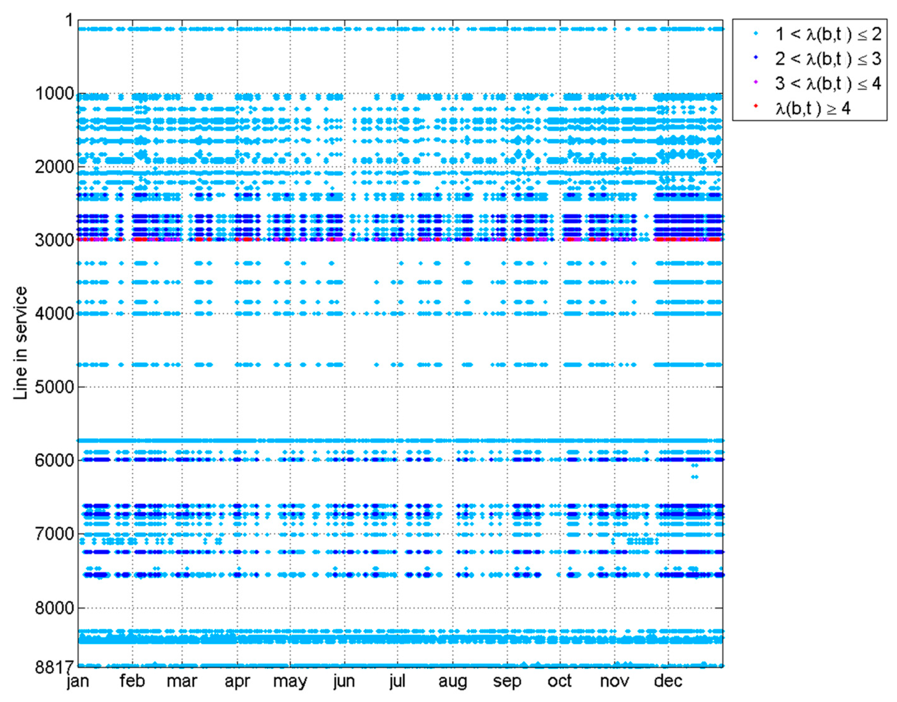
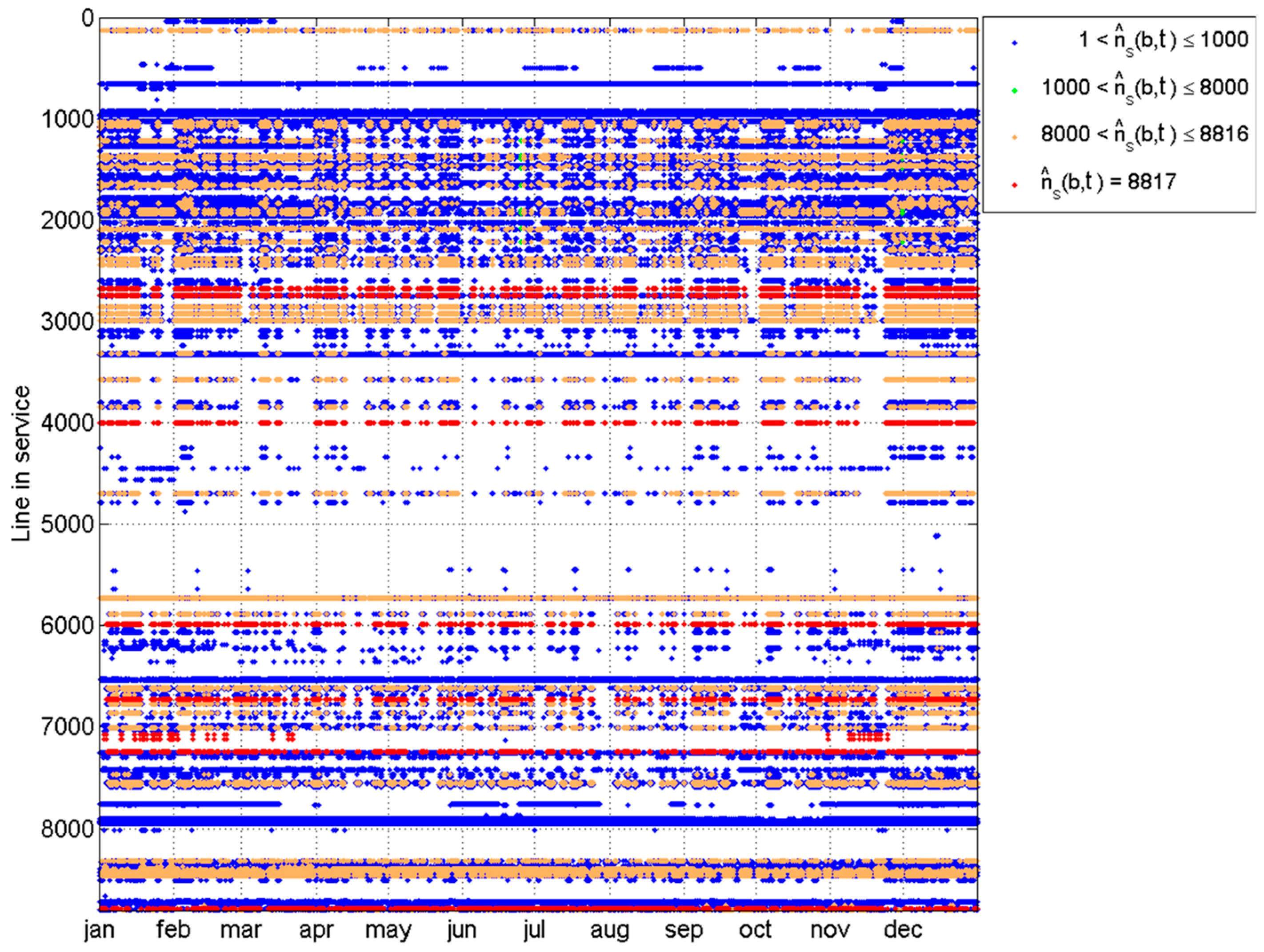
The graphical representation of the $N_b\times N_t$ matrix $\mathbf{\Lambda }$ of yearly loading conditions in the absence of contingencies, obtained by means of PDTFs, and with 77.2 × 10⁶ cases (8817 lines × 8760 h), is reported in Figure 3, where overload cases are represented by markers whose different colors represent overload intensity levels. It can be deduced that the network is interested by slight N overloads affecting a limited set of lines, although no overload is detected in 68 h only.

A synthesis of performance indices is reported in

Table 2. Characterization of yearly network performances in the N condition.

Index	Value
Total overload occurrences	192.5 × 103
Total number of lines affected by overload	132
Maximum $n_q\left(t\right)$	74
Maximum ${\lambda }_q\left(t\right)$	2.25
Maximum $n_t\left(b\right)$	5888

. It can be seen that the total number of overloads corresponds to the 0.25% of the total combinations line-hour, affecting only 1.5% of lines. A particular focus should be given to extreme conditions, registered at hours 849–852 for maximum $n_q\left(t\right)$ and for lines 2992–2993, pertaining to Voltage Range C, for maximum $n_t\left(b\right)$. Maximum ${\lambda }_q\left(t\right)$ is observed at hour 5773 for 23 lines.

Values of the indices by voltage range are reported in

Table 3. Characterization of overloaded lines in the N condition by voltage range.

Voltage Range $\mathit{v}$	$\mathit{a}\left(\mathit{v}\right)$	$\mathit{n}\left(\mathit{v}\right)$	$\mathit{\lambda }\left(\mathit{v}\right)$	${\mathit{a}}_1\left(\mathit{v}\right)$	${\mathit{a}}_2\left(\mathit{v}\right)$
A	63	605	1.14	58	4
B	60	2017	1.62	26	3
C	9	3702	2.12	0	7

, where the number of branches in overload for less than 15% of the year $a_1\left(v\right)$ and the number of branches with average overload higher than 1.2 p.u. $a_2\left(v\right)$ are reported as well. It can be observed that overloaded lines in Range A are 2.2% of the total number, but they show sporadic overloads, since only 5 of them are in overload for more than 15% of the year. Lines in Range A have low overloads as well; considering a 1.2 p.u. overload as acceptable in planning standards [49,50], only 4 lines are troubling. On the other hand, the 9 focused lines in Range C are subject to overloads for more than 40% of hours on average, and with a mean loading value higher than 2. Lines in Range B show an intermediate behavior in each aspect.

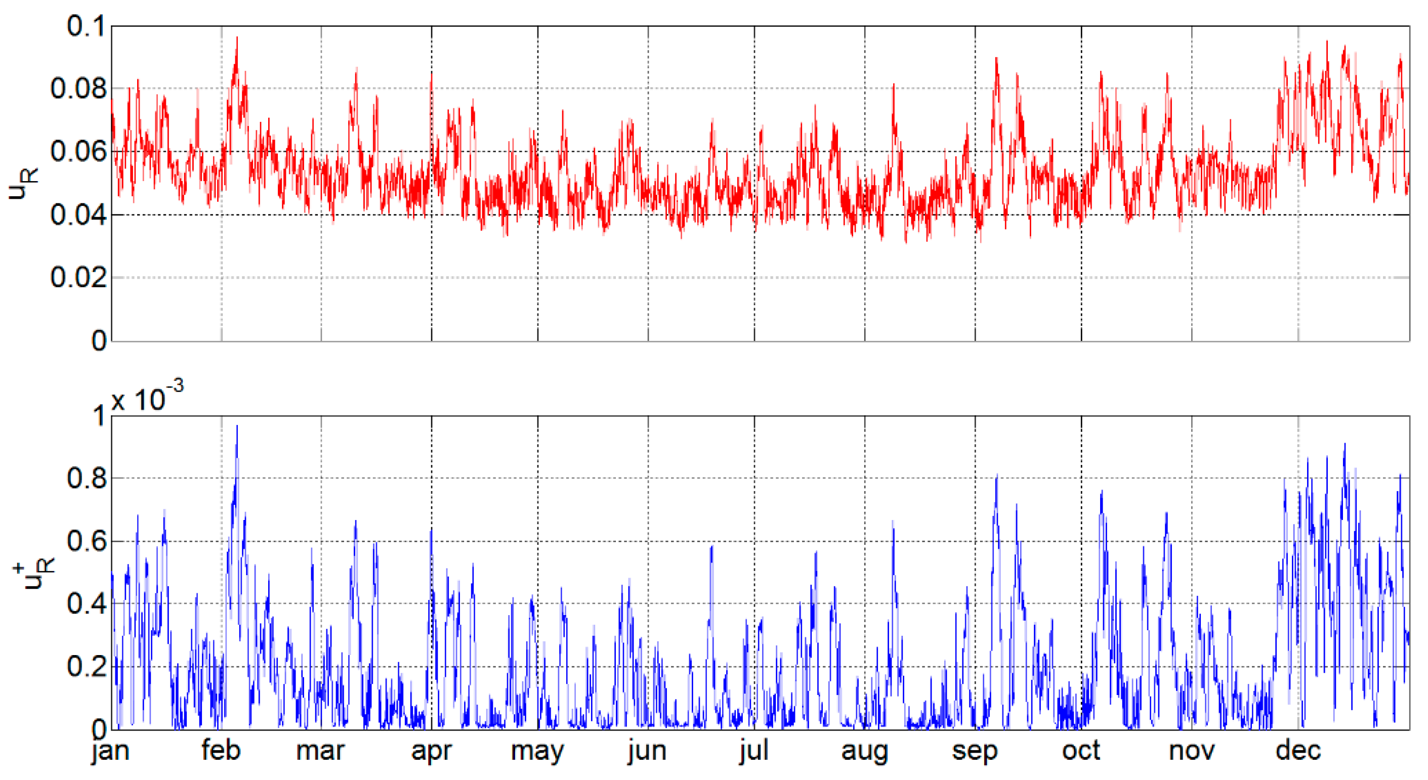
For global network analysis, given that the sum of the ratings of all lines ${\displaystyle \sum }_{b}r\left(b\right)$ is equal to 26.2 GW, trends of indices are reported in Figure 4. It can be noted that $u_R\left(t\right)$ ranges between 3.1% and 9.6% (maximum at hour 849), with an average of 5.4%, resulting in a weakly charged network. This conforms to the assumptions of the method, based on DC power flow equations. On the other hand, $u_R^{+}\left(t\right)$ reaches a maximum of 0.097% at hour 848, although the mean value is 0.0190%, the median value is 0.0133% and the 90-percentile is 0.0491%, highlighting good performances.

3.2. Yearly Operation–N−1 Conditions

The N−1 analysis is therefore carried out by means of the LODF matrix, and the $N_b\times N_b\times N_t$ loading matrix $\widehat{\mathbf{\Lambda }}$ is obtained. It is worthwhile to mention that 1583 cases of N−1 islanding are detected, i.e., 18% of total outages, and they are efficiently dealt with through the developed procedure.

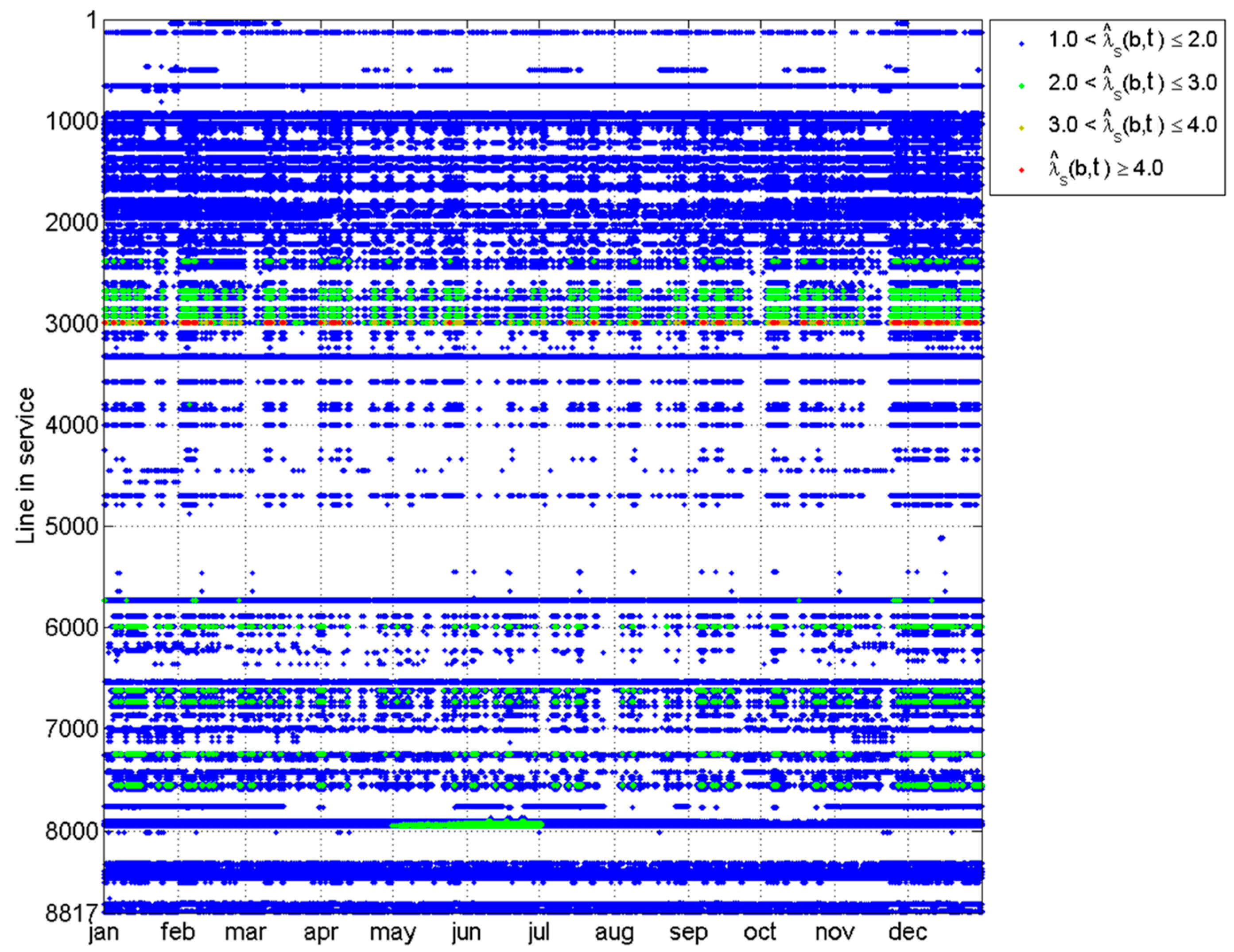
According to the definition of indices in Section 2.3, for the sake of representation, the values of ${\widehat{n}}_s\left(b,h\right)$ and ${\widehat{\lambda }}_s\left(b,h\right)$ are depicted in Figure 5 and Figure 6, respectively, representing the values assumed by the indices in 77.2 × 10⁶ cases. It can be derived that at least one N−1 overload in each hour is registered for 9 lines (rows full of markers in Figure 5 and Figure 6).

The summary of indices is reported in

Table 4. Yearly network performances in N−1 condition (lines in service–hours).

Index	Value
Total overload occurrences	669 × 103
Total number of lines affected by overload	340
Maximum ${\widehat{n}}_q\left(t\right)$	195
Maximum ${\widehat{\lambda }}_q\left(t\right)$	1.57
Maximum ${\widehat{\lambda }}_j\left(b\right)$	2.41
Number of cases with ${\widehat{n}}_s\left(b,t\right)=8817$	40.0 × 103
Number of cases with ${\widehat{\lambda }}_s\left(b,t\right)\ge 2$	48.7 × 103

. It can be noted that N−1 overloads are seen in 0.8% of branch-hour combinations (the total number of markers reported in Figure 5 and Figure 6), and affect 3.8% of branches. Moreover, the cases with overload for the maximum number of outages—i.e., when ${\widehat{n}}_s\left(b,t\right)$ reaches the maximum value of 8817 (red markers in Figure 5)—are detected in 5.9% of total overload cases, affecting 12 lines, mostly in Voltage Range B. The maximum level of ${\widehat{n}}_q\left(t\right)$ is registered at hour 851, and the maximum level of ${\widehat{\lambda }}_t\left(b\right)$ is observed for lines 2992–2993. Regarding overload intensity, ${\widehat{\lambda }}_s\left(b,h\right)\ge 2$ is registered for 7.3% of total overloads, affecting 31 lines, whereas the maximum levels of ${\widehat{\lambda }}_j\left(b\right)$ have analogous features of maximum ${\lambda }_j\left(b\right)$.

Regarding time distribution, from Figure 6 it stems that, for lines with identifier 2500–3000 and 6500–7000, in Ranges B and C, higher overloads are registered in December, January and February, whereas the critical period for lines with identifier 7500–7800, in Range B, is between May and June.

In

Table 5. Characterization of overloaded lines in the N−1 condition.

Voltage Range $\mathit{v}$	$\widehat{\mathit{a}}\left(\mathit{v}\right)$	$\widehat{\mathit{n}}\left(\mathit{v}\right)$	$\widehat{\mathit{\lambda }}\left(\mathit{v}\right)$	${\widehat{\mathit{a}}}_1\left(\mathit{v}\right)$	${\widehat{\mathit{a}}}_2\left(\mathit{v}\right)$	${\widehat{\mathit{e}}}_1\left(\mathit{v}\right)$	${\widehat{\mathit{e}}}_2\left(\mathit{v}\right)$
A	174	1400	1.11	94	8	1381	145
B	135	2284	1.38	66	43	3462	90
C	31	3792	1.68	12	18	2500	22

, the analysis of the 340 lines in N−1 overload by voltage range is reported. Further to indices analogous to the ones proposed in the N condition (see Table 3), the average number of N−1 events causing and overload ${\widehat{e}}_1\left(v\right)$ is estimated, whereas ${\widehat{e}}_2\left(v\right)$ represents the number of lines of the $v$th voltage range with average ${\widehat{n}}_s\left(b,t\right)$ lower than 10% of total N−1 events.

It can be seen that the increase of overloaded lines is most evident in Range A, where more than 6% of lines are affected. However, it is confirmed that higher voltage levels experience less frequent and less intense overloads, seldom reaching remarkable peaks, as compared to Range C.

For N−1 global network indices, no remarkable difference is seen between $u_R\left(t\right)$ and ${\widehat{u}}_R\left(t\right)$. Moreover, ${\widehat{u}}_R^{+}\left(t\right)$ has an average of 0.106%, and a maximum of 0.338% at hour 849, its median is 0.0849%, and its 90-percentile is 0.2165%. These values can be acceptable in N−1 planning, considering the probability of events [51]. 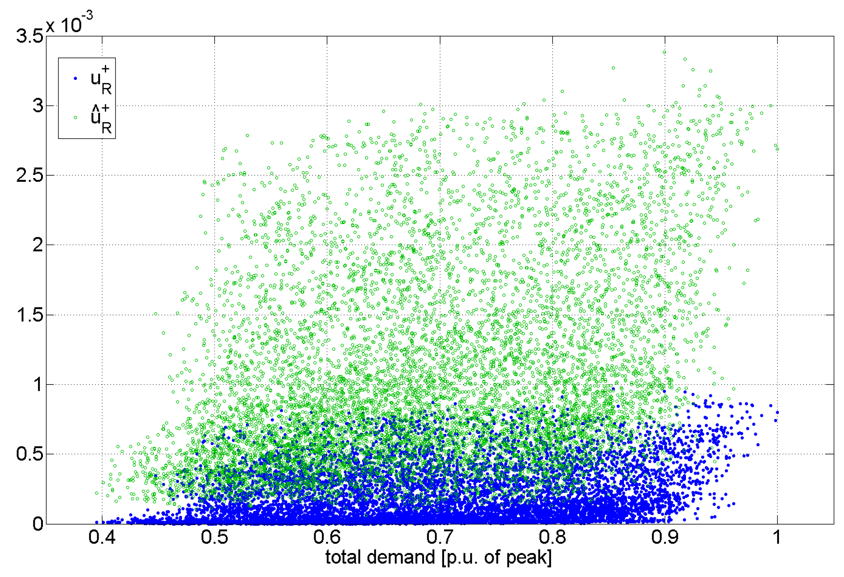Distributions of $u_R^{+}\left(t\right)$ and ${\widehat{u}}_R^{+}\left(t\right),$ with respect to total network demand (between 107.7 MW at hour 8107 and 272.4 MW at hour 3846), are shown in Figure 7. As expected, it can be seen that N−1 events make overloads increase, although severe conditions are not linked to maximum demand (values higher than the 90-percentile are also seen for half of the peak load). This can be ascribed to the load distribution among zones.

In

Table 6. Yearly network performances in the N−1 condition (lines in outage–hours).

Index	Value
Total overload occurrences	76.6 × 106
Maximum ${\widehat{n}}_c\left(k,t\right)$	84
Maximum ${\widehat{\lambda }}_c\left(k,t\right)$	2.43
Number of cases with ${\widehat{\lambda }}_c\left(k,t\right)\ge 2$	2.25 × 106

, the analysis of indices by outage-hour, ${\widehat{n}}_c\left(k,t\right)$ and ${\widehat{\lambda }}_c\left(k,t\right)$, is synthesized. Overloads are seen in the majority of outage cases. The maximum number of N−1 overloads ${\widehat{n}}_c\left(k,t\right)$ is 84, observed at hour 849 for the outage of line 1036, in Voltage Range A, whereas the maximum ${\widehat{\lambda }}_c\left(k,t\right)$ of 2.43 is seen for the outage of line 2924 at hour 2842, and values of ${\widehat{\lambda }}_c\left(k,t\right)\ge 2$ are reached in 2.9% of total overloads.

Hourly analysis by means of indices ${\widehat{n}}_h\left(b,k\right)$ and ${\widehat{\lambda }}_h\left(b,k\right)$ is carried out on 77.7 × 10⁶ cases (8817 lines × 8817 lines), and reported in

Table 7. Yearly network performances in N−1 condition (lines in service–lines in outage).

Index	Value
Total overload occurrences	1.165 × 106
Total number of lines affected by overload	340
Number of cases with ${\widehat{n}}_h\left(b,k\right)\ge 8000$	13
Number of cases with ${\widehat{\lambda }}_h\left(b,k\right)\ge 2$	35.3 × 103

. It can be deduced that N−1 overloads are observed in 1.5% of total cases. The 132 lines in overload in the N condition experience N−1 overload for more than 8600 outages. Moreover, N−1 overload is present in 191 lines for less than 10 outages, in 11 lines for a range of 10 to 100 events and in 6 lines for 100 to 600 outages. As regards the values of indices, 31 lines in service have ${\widehat{n}}_h\left(b,k\right)>3000$ for almost all outages, whereas other 68 lines are interested by ${\widehat{n}}_h\left(b,k\right)>3000$ in less than 20 N−1 events. Only in 13 cases, each affecting a single line in service, is ${\widehat{n}}_h\left(b,k\right)>8000$ is observed. Values of ${\widehat{\lambda }}_h\left(b,k\right)\ge 2$ are present in 3% of overloads, affecting 4 branches in any N−1 event, and another 16 branches in less than 5 outages, but only in 7 cases is a ${\widehat{\lambda }}_h\left(b,k\right)\ge 3$ observed.

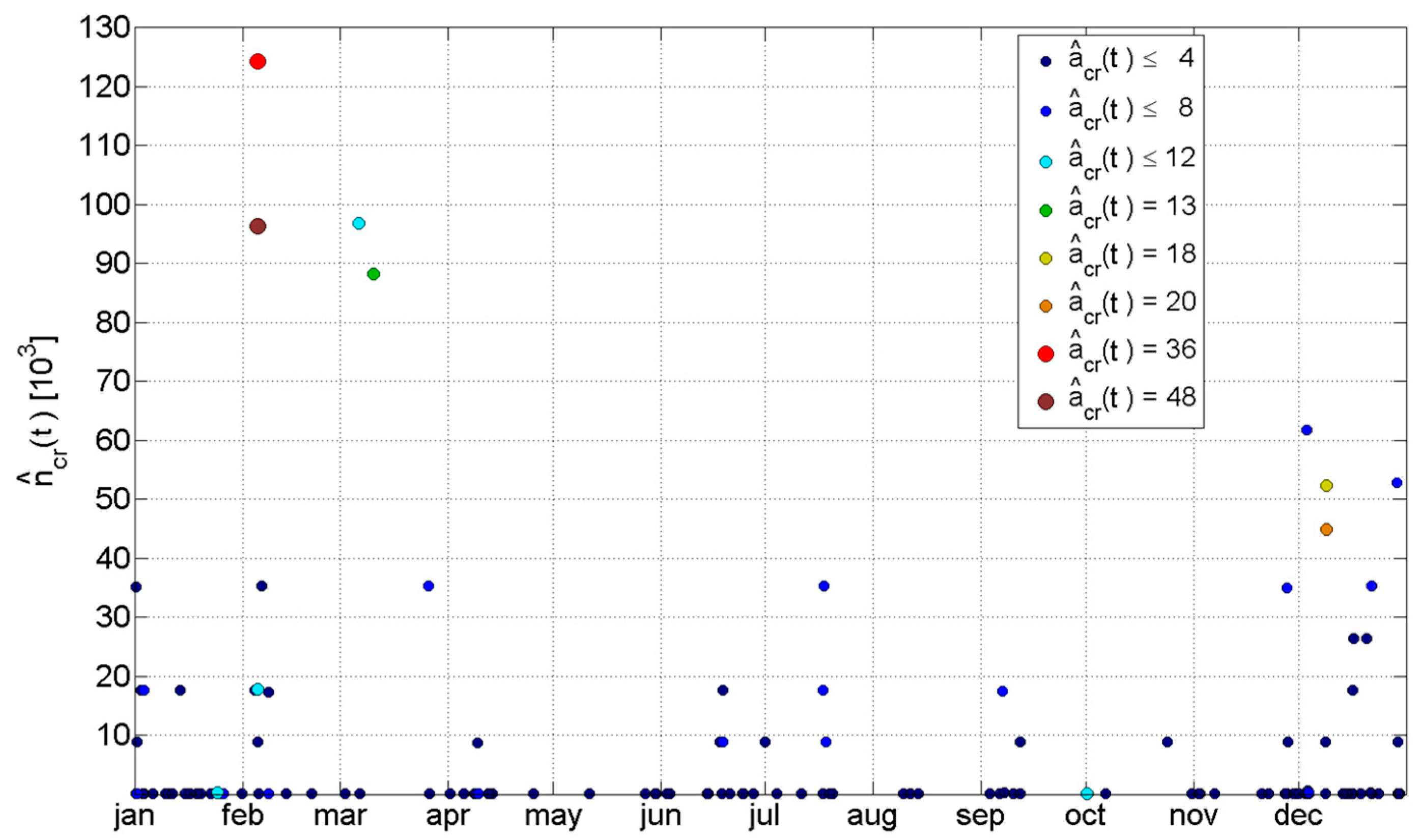
In order to individuate the most troubling conditions, for each couple line in service–line in outage (i.e., $b, k$), the hour with the maximum ${\lambda }^{+}\left(b,k,t\right)$, defined as critical overload, is found. The occurrences of critical overloads in each hour ${\widehat{n}}_{cr}\left(t\right)$ are reported in Figure 8, where the bullet color represents the number of lines affected by critical overloads in that hour ${\widehat{a}}_{cr}\left(t\right)$. Critical overloads are detected in 144 h (total number of markers in Figure 8), mostly in winter. The highest number is 124.4 × 10³ for hour 848 (10.7% of the total), whereas the maximum number of 48 lines with critical overload is registered in hour 849. This last hour is the most critical condition for different aspects, deserving a detailed analysis in the next subsection.

3.3. Analysis of Specific Loading Condition

The line loading levels in the N condition at hour 849 show that 74 lines are in overload in the N condition, and 22 of them, in Ranges B and C, have $\left(b,849\right)>2$. The global network performance is described by $u_R\left(849\right)$ = 9.63% and $u_R^{+}\left(849\right)$ = 0.095%.

As regards N−1 analysis, involving 77.7 × 10⁶ cases, synthetic indices are reported in

Table 8. Network performances in N−1 at hour 849 (lines in service–outages).

Index	Value
Total overload occurrences	653.7 × 103
Total number of lines affected by overload	193
Number of cases with $\widehat{\lambda }\left(b,k,849\right)\ge 5$	6
Number of cases with $\widehat{\lambda }\left(b,k,849\right)\ge \lambda \left(b,849\right)$	187.3 × 103

. Overloads are observed in 0.8% of combinations, affecting 193 lines. Peak overloads, with $\widehat{\lambda }\left(b,h,849\right)\ge 5$, are detected only in 6 lines due to outages close to lines already overloaded in the N condition. In 28.6% of the overloads, the amount of N−1 overload is higher than the overload in the N condition, affecting in particular lines 8432 and 8433, in Voltage Range B. Moreover, global N−1 performances are described through the index ${\widehat{u}}_R^{+}\left(849\right)$= 0.338%.

In

Table 9. Distribution of average N−1 overloads at hour 849.

Class of ${\widehat{\mathit{\lambda }}}_{\mathit{s}}\left(\mathit{b},849\right)$	Number of Lines
(1.0, 1.2]	106
(1.2, 1.8]	64
(2.0, 2.8]	19
(3.6, 4.2]	4

, average N−1 overloads ${\widehat{\lambda }}_s\left(b,849\right)$ are divided into classes. More than half of overloaded lines have ${\widehat{\lambda }}_s\left(b\right)\le 1.2$, considered acceptable in N−1 network planning as described in the above, whereas 23 lines, mostly in overload in the N condition, show values higher than 2.

The number of lines in overload due to the outage of line $k$, ${\widehat{n}}_c\left(k,849\right)$, is detailed in

Table 10. Distribution of the number of overloaded lines in N−1 condition at hour 849.

Class of ${\widehat{\mathit{n}}}_{\mathit{c}}\left(\mathit{k},849\right)$	Number of Occurrences
70 ÷ 73	69
74	8082
75 ÷ 79	642
80 ÷ 84	24

. In 91.7% of outages, the number of overloaded lines is the same as in the N condition. The maximum of 84 overloads is observed for the outage of lines 1035 and 1036, in Voltage Range A, arising as the most critical lines for N−1 analysis in this hour. Moreover, 9 lines are in overload for any outage, whereas for 44 lines, only 1 outage induces an overload.

The performed investigation allows an early detection of critical lines, which could represent the target of a specific security analysis during operational planning, along with risk measures depending on device failure rates and further technical details.

4. Conclusions

A flow-based procedure for the preliminary security analysis of a yearly network evolution scenario has been proposed. Starting from hourly load and generation by market solution, linear PTDFs and LODFs have been exploited to assess N and N−1 power flows and loading levels. In particular, an extended matrix formulation has been carried out to efficiently handle N−1 islanding. Statistic indices have been defined to inspect network behavior in the big data framework. The procedure has been tested on a model of provisional European high voltage network involving thousands of nodes and lines. Simulations have proved the effectiveness of the tool to handle a real-sized network with a plain formulation, and to point out the security effects of varying loading conditions and events, suiting multiple post-elaborations. The proposed method has proved to be a powerful and flexible tool for TSO long-term and secure operation analysis, even in the presence of a remarkable amount of data, leading to point out critical conditions to be further inspected during system operation, and critical branches to evaluate grid developments. The tool could be useful for other entities involved in power systems as well, such as generation companies, traders and regulators, in order to draw, by means of the defined indicators, useful technical-based signals to evaluate new initiatives or strategies in energy and service markets. Future work could aim at regulation strategies for reducing overloads, and at their application to network expansions.

References

1. Dijkstra, S.; Gaxiola, E.; Nieuwenhout, F.; Orfanos, G.; Ozdemir, Ö.; van der Welle, A. European scenario synthesis to be used for electricity transmission network planning. In Proceedings of the 2012 EEM International Conference, Florence, Italy, 10–12 May 2012; pp. 1–5. [Google Scholar] [CrossRef]
2. Fürsch, M.; Hagspiel, S.; Jägermann, C.; Nagl, S.; Lindenberger, D.; Tröster, E. The role of grid extensions in a cost-efficient transformation of the European electricity system until 2050. Appl. Energy 2013, 104, 642–652. [Google Scholar] [CrossRef] [Green Version]
3. Escobar, L.; Romero, R.; Escobar, A.; Gallego, R. Long term transmission expansion planning considering generation-demand scenarios and HVDC lines. In Proceedings of the IEEE PES T&D-LA Conference, Morelia, Mexico, 20–24 September 2016; pp. 1–6. [Google Scholar] [CrossRef]
4. Lumbreras, S.; Ramos, A. The new challenges to transmission expansion planning. Survey of recent practice and literature review. Electr. Power Syst. Res. 2016, 134, 19–29. [Google Scholar] [CrossRef]
5. Krishnan, V.; Ho, J.; Hobbs, B.F.; Liu, A.L.; McCaley, J.D.; Shahidehpour, M.; Zheng, Q.P. Co-optimization of electricity transmission and generation resources for planning and policy analysis: Review of concepts and modeling approaches. Energy Syst. 2016, 7, 297–332. [Google Scholar] [CrossRef]
6. Jaehnert, S.; Wolfgang, O.; Farahmand, H.; Völler, S.; Huertas-Hernando, D. Transmission expansion planning in Northern Europe in 2030—Methodology and analyses. Energy Policy 2013, 61, 125–139. [Google Scholar] [CrossRef]
7. Koltsaklis, N.E.; Dagoumas, A.S.; Georgiadis, M.C.; Papaioannou, G.; Dikaiakos, C. A mid-term, market-based power systems planning model. Appl. Energy 2016, 179, 17–35. [Google Scholar] [CrossRef]
8. Munoz, F.D.; Hobbs, B.F.; Ho, J.L.; Kasina, S. An engineering-economic approach to transmission planning under market and regulatory uncertainties: WECC case study. IEEE Trans. Power Syst. 2014, 29, 307–317. [Google Scholar] [CrossRef]
9. Rahmani, M.; Kargarian, A.; Hug, G. Comprehensive power transfer distribution factor model for large-scale transmission expansion planning. IET Gen. Transm. Distrib. 2016, 10, 2981–2989. [Google Scholar] [CrossRef]
10. Åmellem, L.; Kristiansen, M.; Korpås, M. Incorporation of flow-based grid modelling in multinational transmission expansion planning. In Proceedings of the 15th Wind Integration Workshop, Vienna, Austria, 15–17 November 2016; pp. 1–6. [Google Scholar]
11. Moreira, A.; Street, A.; Arroyo, J.M. An adjustable robust optimization approach for contingency-constrained transmission expansion planning. IEEE Trans. Power Syst. 2015, 30, 2013–2022. [Google Scholar] [CrossRef]
12. Spieker, S.; Schwippe, J.; Klein, D.; Rehtanz, C. Transmission system congestion analysis based on a European electricity market and network simulation framework. In Proceedings of the 2016 PSCC Conference, Genoa, Italy, 20–24 June 2016; pp. 1–7. [Google Scholar] [CrossRef]
13. Bo, R.; Wu, C.; Yan, J.; Hecker, L.; Zhou, Z. LODF-based transmission solution screening method in economic transmission planning. In Proceedings of the 2015 IEEE PES GM, Denver, CO, USA, 26–30 July 2015; pp. 1–5. [Google Scholar] [CrossRef]
14. Wood, A.; Wollenberg, B.; Sheblé, G. Power Generation, Operation, and Control, 3rd ed.; John Wiley & Sons, Inc.: Hoboken, NJ, USA, 2014. [Google Scholar]
15. Güler, T.; Gross, G.; Liu, M. Generalized Line Outage Distribution Factors. IEEE Trans. Power Syst. 2007, 22, 879–881. [Google Scholar] [CrossRef]
16. Fu, Y.; Li, Z. A Direct Calculation of Shift Factors Under Network Islanding. IEEE Trans. Power Syst. 2015, 30, 1550–1551. [Google Scholar] [CrossRef]
17. Ronellenfitsch, H.; Timme, M.; Witthaut, D. A Dual Method for Computing Power Transfer Distribution Factors. IEEE Trans. Power Syst. 2007, 32, 1007–1015. [Google Scholar] [CrossRef] [Green Version]
18. Majidi-Qadikolai, M.; Baldick, R. Integration of N − 1 contingency analysis with systematic transmission capacity expansion planning: ERCOT Case Study. IEEE Trans. Power Syst. 2016, 31, 2234–2245. [Google Scholar] [CrossRef]
19. Hinojosa, V.H.; Velásquez, J. Improving the mathematical formulation of security-constrained generation capacity expansion planning using power transmission distribution factors and line outage distribution factors. Electr. Power Syst. Res. 2016, 140, 391–400. [Google Scholar] [CrossRef]
20. Goldis, E.A.; Caramanis, M.C.; Philbrick, C.R.; Rudkevich, A.M.; Ruiz, P.A. Security-constrained MIP formulation of topology control using loss-adjusted shift factors. In Proceedings of the 2014 47th Hawaii International Conference on System Science, Waikoloa, HI, USA, 6–9 January 2014; pp. 2503–2509. [Google Scholar] [CrossRef]
21. Li, S.; Han, X.; Wang, M.; Wang, Y.; Zhang, Q. A new method for reference network considering contingent events based on line outage distribution factor. In Proceedings of the 2016 TENCON Conference, Singapore, 22–25 November 2016; pp. 542–545. [Google Scholar] [CrossRef]
22. Gutierrez-Alcaraz, G.; Gonzalez-Cabrera, N.; Gil, E. An efficient method for Contingency-Constrained Transmission Expansion Planning. Electr. Power Syst. Res. 2020, 182, 106208. [Google Scholar] [CrossRef]
23. Mehrtash, M.; Kargarian, A.; Rahmani, M. Security-constrained transmission expansion planning using linear sensitivity factors. IET Gener. Trans. Distrib. 2020, 14, 200–210. [Google Scholar] [CrossRef]
24. Matthes, B.; Spieker, C.; Rehtanz, C. Flow-Based Parameter Determination in Large-Scale Electric Power Transmission System. In Proceedings of the 2017 IEEE Manchester PowerTech, Manchester, UK, 18–22 June 2017; pp. 1–6. [Google Scholar] [CrossRef]
25. Dehghanian, P.; Kezunovic, M. Probabilistic decision making for the bulk power system optimal topology control. IEEE Trans. Smart Grid 2016, 7, 2071–2081. [Google Scholar] [CrossRef]
26. Hinojosa, V.H. Comparing Corrective and Preventive Security-Constrained DCOPF Problems Using Linear Shift-Factors. Energies 2020, 13, 516. [Google Scholar] [CrossRef] [Green Version]
27. Tejeda-Arango, D.A.; Sánchez-Martin, P.A. Ramos, Security Constrained Unit Commitment Using Line Outage Distribution Factors. IEEE Trans. Power Syst. 2018, 33, 329–337. [Google Scholar] [CrossRef]
28. Retty, H.; Thorp, J.S.; Centeno, V. The Effect of Load Model Composition on N−1 Contingency Ranking. In Proceedings of the 2015 IEEE PES ISGT Conference, Washington, DC, USA, 18–20 February 2015; pp. 1–5. [Google Scholar] [CrossRef]
29. Dourbois, G.A.; Biskas, P.N.; Chatzigiannis, D.I.; Vlachos, A.G.; Bakirtzis, A.G. European day-ahead market clearing model incorporating linearized AC power flow constraints. In Proceedings of the 2016 PSCC Conference, Genoa, Italy, 20–24 June 2016; pp. 1–7. [Google Scholar] [CrossRef]
30. Ullah, I.; Gawlik, W.; Palensky, P. Analysis of power network for line reactance variation to improve total transmission capacity. Energies 2016, 9, 936. [Google Scholar] [CrossRef]
31. Kezunovic, M.; Xie, L.; Grijalva, S. The Role of Big Data in Improving Power System Operation and Protection. In Proceedings of the 2013 IREP Symposium, Rethymnon, Greece, 25–30 August 2013; pp. 1–9. [Google Scholar] [CrossRef]
32. Bessa, R.J. Future trends for big data application in power systems. In Big Data Application in Power Systems; Arghandeh, R., Zhou, Y., Eds.; Elsevier Inc.: Amsterdam, The Netherlands, 2018. [Google Scholar] [CrossRef]
33. Zhang, Y.; Huang, T.; Bompard, E.F. Big data analytics in smart grids: A review. Energy Inf. 2018, 1, 8. [Google Scholar] [CrossRef]
34. Franken, M.; Schrief, A.B.; Barrios, H.; Schnettler, A. Network Reinforcement Applying Redispatch-based Indicators. In Proceedings of the 2018 53rd UPEC International Conference, Glasgow, UK, 4–7 September 2018; pp. 1–6. [Google Scholar] [CrossRef]
35. Ha, D.T.; Retière, N.; Caputo, J.-G. A New Metric to Quantify the Vulnerability of Power Grids. In Proceedings of the 2019 ICSSE International Conference, Dong Hoi, Vietnam, 20–21 July 2019; pp. 206–213. [Google Scholar] [CrossRef]
36. Long, C.; You, D.; Hu, J.; Wang, G.; Dong, M. Quick and effective multiple contingency screening algorithm based on long-tailed distribution. IET Generat. Trans. Distribut. 2016, 10, 257–262. [Google Scholar] [CrossRef]
37. Güler, T.; Gross, G. Detection of island formation and identification of causal factors under multiple line outage. IEEE Trans. Power Syst. 2007, 22, 505–513. [Google Scholar] [CrossRef]
38. Farrokhabadi, M.; Vanfretti, L. An efficient automated topology processor for state estimation of power transmission networks. Electr. Power Syst. Res. 2014, 106, 188–202. [Google Scholar] [CrossRef]
39. Hazarika, D.; Bhuyan, S.; Chowdhury, S.P. Line outage contingency analysis including the system islanding scenario. Int. J. Electr. Power Energy Syst. 2006, 28, 232–243. [Google Scholar] [CrossRef]
40. Velay, M.; Vinyals, M.; Besanger, Y.; Retiere, N. Fully distributed security constrained optimal power flow with primary frequency control. Int. J. Electr. Power Energy Syst. 2019, 110, 536–547. [Google Scholar] [CrossRef] [Green Version]
41. Pinto, H.; Magnago, F.; Brignone, S.; Alsaç, O.; Stott, B. Security Constrained Unit Commitment: Network Modeling and Solution Issues. In Proceedings of the 2006 IEEE PES Power Systems Conference and Exposition, Atlanta, GA, USA, 29 October–1 November 2006; pp. 1–6. [Google Scholar] [CrossRef]
42. Chen, Y.; Zhang, Z.; Liu, Z.; Zhang, P.; Ding, Q.; Liu, X.; Wang, W. Robust N-k CCUC model considering the fault outage probability of units and transmission lines. IET Generat. Trans. Distribut. 2019, 13, 3782–3791. [Google Scholar] [CrossRef]
43. Conejo, A.J.; Morales, L.B.; Kazempour, S.J.; Siddiqui, A.S. Investment in Electricity Generation and Transmission; Springer: Cham, Switzerland, 2016. [Google Scholar] [CrossRef] [Green Version]
44. AlAli, D.; Griffiths, H.; Cipcigan, L.M.; Haddad, A. Assessment of Line Overloading Risk for Transmission Networks. In Proceedings of the 11th IET International Conference on AC and DC Power Transmission, Birmingham, UK, 10–12 Feberuary 2015. [Google Scholar] [CrossRef]
45. ENTSO-E. Ten Years Network Development Plan 2018 Data; ENTSO-E: Brussels, Belgium, 2018; Available online: https://tyndp.entsoe.eu/maps-data/ (accessed on 10 December 2019).
46. Zimmerman, R.D.; Murillo-Sánchez, C.E.; Thomas, R.J. MATPOWER: Steady-state operations, planning, and analysis tools for power systems research and education. IEEE Trans. Power Syst. 2011, 26, 12–19. [Google Scholar] [CrossRef] [Green Version]
47. Aluisio, B.; Forte, G.; Dicorato, M.; Trovato, M.; Sallati, A.; Gadaleta, C.; Vergine, C.; Ciasca, F. The application of a flow based methodology for yearly network analysis according to market data. In Proceedings of the 2017 14th International Conference on the European Energy Market (EEM), Dresden, Germany, 6–9 June 2017; pp. 1–6. [Google Scholar] [CrossRef]
48. Allegretti, A.; Forte, G.; Dicorato, M.; Trovato, M.; Aluisio, B.; Gadaleta, C.; Vergine, C. Phase Shifting Transformer in flow-based yearly network analysis for European market envision. In Proceedings of the 2018 15th International Conference on the European Energy Market (EEM), Lodz, Poland, 27–29 June 2018; pp. 1–6. [Google Scholar] [CrossRef]
49. MED-TSO. EC DEVCO—Grant Contract: ENPI/2014/347-006 Mediterranean Project, Deliverable 2.1.1 Guidelines for Coordinated Planning: (B) Survey and Tools for Supporting the Harmonized Planning Process; MED-TSO: Rome, Italy, 2015; Available online: www.med-tso.com (accessed on 20 October 2019).
50. Joint Working Group CIGRE/CIRED C1.29. Planning Criteria for Future Transmission Networks in the Presence of a Greater Variability of Power Exchange with Distribution Systems; CIGRE: Paris, France, 2017; ISBN 978-2-85873-384-2. [Google Scholar]
51. Li, X.; Zhang, X.; Wu, L.; Lu, P.; Zhang, S. Transmission line overload risk assessment for power systems with wind and load-power generation correlation. IEEE Trans. Smart Grid 2015, 6, 1233–1242. [Google Scholar] [CrossRef]
Figure 1. Statistical analysis applied to the N−1 overload matrix.
Energies 13 03363 g001
Figure 2. Perimeter of provisional network under investigation.
Energies 13 03363 g002
Figure 3. Line loading in the N condition for the yearly operation.
Energies 13 03363 g003
Figure 4. Network loading indices in the N condition for the yearly operation.
Energies 13 03363 g004
Figure 5. N−1 overloads for each line in each hour of yearly operation.
Energies 13 03363 g005
Figure 6. Average amount of N−1 overloads for each line in yearly operation.
Energies 13 03363 g006
Figure 7. Distribution of N and N−1 network overload indices with respect to total demand.
Energies 13 03363 g007
Figure 8. Individuation of the most critical hours in the N−1 analysis.
Energies 13 03363 g008