Continuous Control Set Model Predictive Control of a Switch Reluctance Drive Using Lookup Tables

Abstract

A problem of the switched reluctance drive is its natural torque pulsations, which are partially solved with finite control set model predictive control strategies. However, the continuous control set model predictive control, required for precise torque stabilization and predictable power converter behavior, needs sufficient computation resources, thus limiting its practical implementation. The proposed model predictive control strategy utilizes offline processing of the magnetization surface of the switched reluctance motor. This helps to obtain precalculated current references for each torque command and rotor angular position in the offline mode. In online mode, the model predictive control strategy implements the current commands using the magnetization surface for fast evaluation of the required voltage command for the power converter. The proposed strategy needs only two lookup table operations requiring very small computation time, making instant execution of the whole control system possible and thereby minimizing the control delay. The proposed solution was examined using a simulation model, which showed precise and rapid torque stabilization below rated speed.

1. Introduction

Switched reluctance drives (SRDs) have attracted a significant amount of attention in recent decades as the most promising type of electric drive. With the spread of 3D-printing technologies, this drive is one of the best candidates to become the first commercial 3D-printed machine [1] and modular designed machine [2]. Being very simple, the machine requires a sophisticated control strategy, which currently has no general approach, unlike the field-oriented control (FOC) or direct torque control (DTC) used in AC electric drives. Many papers have considered the mitigation of torque ripple by adjustment of the commutation angles [3,4,5] and current profiles [6,7], or optimization of the motor magnetic geometry [8]. However, solutions suggested in [3,4,5] help in the limited range of speeds as the current slope varies with the speed also affecting the produced torque. Current profiling suggested in [6,7] cannot be applied to each particular motor without hand tuning in all operation modes. In addition, optimization of the magnetic geometry for torque ripple minimization [8] contradicts the goal of efficiency optimization of the electrical machine.

The approach with model predictive control using a finite control set (FCS) was suggested in [9] to help decrease torque ripple and make the control strategy applicable for any motor. It was improved in [10] by decreasing the losses in the motor and in [11] by achieving equal distribution of the temperatures of the power converter’s IGBT-modules. These approaches utilize the magnetization surface of the switched reluctance motor for torque estimation while selecting the best control command. These systems stabilize the output torque by profiling the phase current shape, not only with respect to the commanded torque, but also minimizing ohmic losses. The disadvantage of the finite control set model predictive control is the random switching rate and the error in the commanded torque or speed if a short prediction horizon is used. Continuous control set (CCS) model predictive control solves the voltage equations to obtain the references to the inverter, but this approach is problematic for a switched reluctance machine (SRM) due to the high nonlinearity of the controlled plant as the motor inductance varies with current and the power converter frequently saturates.

During analysis of the model predictive control (MPC) operation it was noticed that, for each electrical revolution for the same torque command, the current references repeat. The cost function, which considers the difference between the commanded and predicted torque, and minimizes ohmic losses, gives the predefined shape of the current references with respect to the rotor position. Together with the magnetization surface of each phase, this can be used to evaluate the desired voltage command, which adjusts the state variables of the drive to follow the references. Compared to the existing methods, the proposed solution uses information about the magnetization map of the machine to obtain the current references for the demanded torque, and then evaluates voltage references using the magnetization surface. The control strategy uses only lookup table operations, which allows evaluation of the voltage command nearly instantly, thus requiring very small computation efforts.

2. Switched Reluctance Drive Model

2.1. Drive Topology

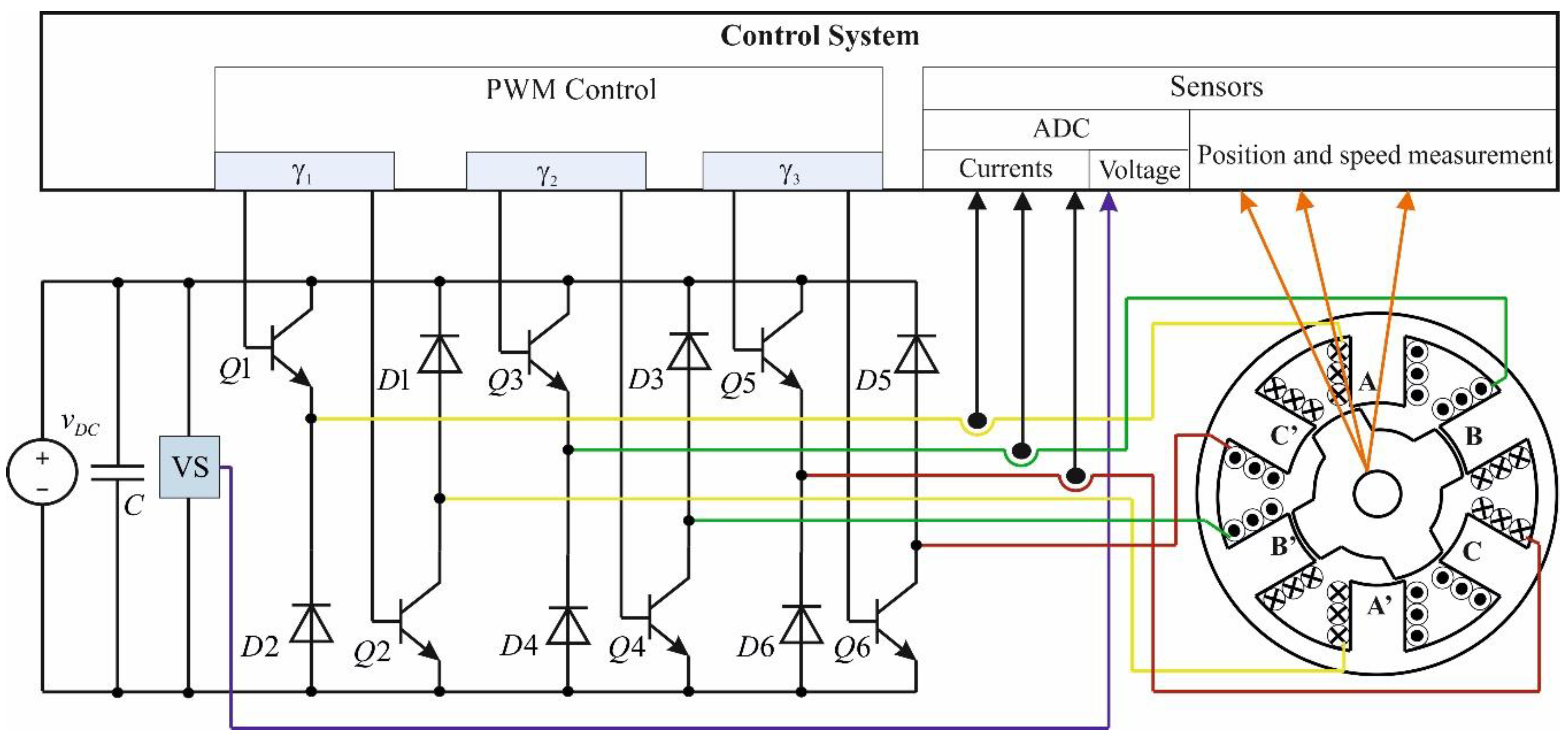
The switched reluctance drive can have a varying number of phases and its power converter topology can vary. The most common configuration of the drive is shown in Figure 1. The stator of the motor contains three phases with concentrated windings located at six stator teeth. The rotor has four teeth, and the electromechanical reduction ratio is 4. The power converter is represented by three asymmetrical H-bridges, which feed the motor phases with unipolar current.

2.2. Motor Equations

Each phase has its voltage balance equation [10]:

$$\frac{\mathrm{d}\mathsf{\psi }}{\mathrm{d}t}=v-iR,$$

(1)

where v is the applied voltage, i is the flowing current, R is the phase resistance, and ψ is the flux linkage of the winding.

The magnetic system of an SRM is highly non-linear, which is usually defined by means of a magnetization surface/map or flux linkage map. For AC machines these maps can be identified online using a testbench that consists of the motor under test and a prime mover motor [12]. This testbench can realize all possible operation conditions and uses high-frequency injection to estimate differential inductance maps in order to build flux linkage maps. Such a method is applicable for SRMs; however, other methods are more popular due to the specific nature of this machine.

The motor phases of an SRM are usually considered to be independent without, or with very little, magnetic coupling between them [11]. Therefore, the magnetization surface of each phase depends on its flowing current and current rotor angular position as shown in Figure 2. The magnetization map of an SRM can be obtained experimentally [12,13]. Paper [12] provides a thorough description of experimental setups for making flux linkage maps. In [13], authors represent two methods of flux linkage map measurement based on the example of a four-phase SRM. The first method utilized a testbench with a mechanical rotor locking device and measured current and voltage. The flux linkage was calculated offline using experimental data. The second method was an online method. It did not require a rotor locking device, and online data from current and voltages sensors were used to evaluate the magnetization map when the SRM was running in a normal operation mode. For the considered solution, the offline method is preferable, as the online method provides an incomplete data set limited by the operation conditions of the drive, which makes estimation of the torque surface impossible.

The torque of the phase at the electrical speed can be defined as a function of the phase energy:

$$T=-\frac{\partial {\displaystyle \underset{0}{\overset{\mathsf{\psi }}{\int }}\mathrm{i}\left(\mathsf{\psi },\mathsf{\theta }\right)\mathrm{d}\mathsf{\psi }}}{\partial \mathsf{\theta }},$$

(2)

or co-energy:

$$T=\frac{\partial {\displaystyle \underset{0}{\overset{i}{\int }}\mathsf{\psi }\left(i,\mathsf{\theta }\right)\mathrm{d}i}}{\partial \mathsf{\theta }},$$

(3)

where θ is the electrical rotor angular position.

The total torque of the machine is the sum of the torques produced by each phase. For a considered motor with number of phases N equal to 3, the torque equation can be written as follows:

$$T={\displaystyle \sum _{n=1}^N{T}_n}=T_1+T_2+T_3.$$

(4)

2.3. Power Converter

Each phase of the motor is connected to the asymmetrical bridge as shown in Figure 1. The phase current can only flow in one direction, which is considered to be the positive direction. It is possible to apply a positive voltage of the DC link by switching on both switches in the bridge, zero voltage by switching on only one of the switches, and negative voltage by switching off both switches. In the last case the phase current flows through freewheeling diodes, and the negative voltage is applied only while the flowing current is bigger than zero.

3. Continuous Control Set Model Predictive Control for SRD

The FCS MPC, which is taken as the reference, was proposed in [10]. The MPC algorithm checked 27 possible states of the power converter and estimated the behaviors of the phase currents and torque for each case. The cost function was developed to keep total torque closer to the reference with minimum ohmic losses in the phase windings.

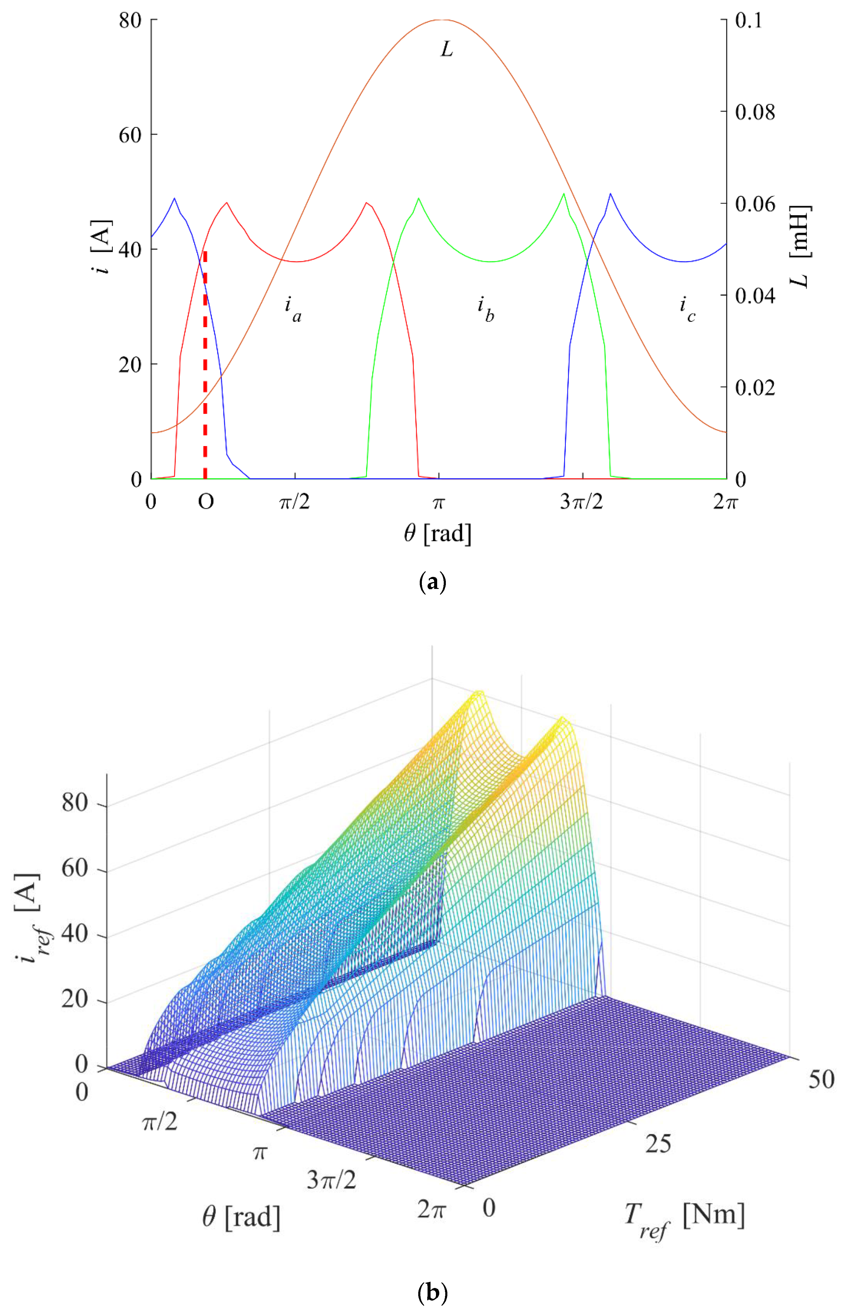
As a result, for the infinite switching rate, the current shape was profiled to achieve nearly constant torque as shown in Figure 3a. The waveform of the phase current contains the period of growing current, when the phase operates together with the previously on phase, which is reaching the point of maximum inductance (aligned position). When the previous phase reaches the aligned position, it is not desirable to keep current in it anymore as it does not produce positive torque. So, the previously on phase turns off, and all the torque, produced by the motor, is delivered to the shaft by a single phase at its second time interval. The current is regulated according to the magnetization surface of the motor to produce the commanded torque. Then, the inductance of this phase reaches its maximum value. Its current is reduced, and the next phase is switched on.

This current waveform is repeated each revolution; therefore, it is possible to evaluate it in advance (offline) for each torque reference.

Having variable rotor angular positions and torque references, the solution for each phase current can be represented as a function of these two variables. This function is easy to implement using a lookup table. An example of the current reference surface for phase A is shown in Figure 3b.

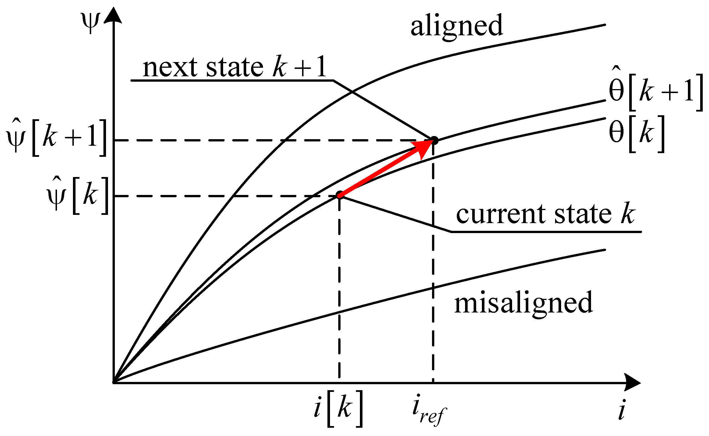
The current regulation can be performed using the magnetization surface of the motor phase. With the rotation of the machine and change of the current reference, the system should move from one point of the surface to another.

At the end of the pulse-width modulation (PWM) cycle, the current is to be measured and the control system should be executed. The control system has information about the measured current i[k] (see Figure 4) and current rotor electrical position θ[k]. Knowing the motor speed ω, the rotor position in the end of the next PWM cycle can be evaluated by:

$$\widehat{\mathsf{\theta }}\left[k+1\right]=\mathsf{\theta }\left[k\right]+\omega \cdot T_{PWM},$$

(5)

where T_PWM is the duration of the PWM cycle.

Knowing the torque reference T_ref, the current reference for the next PWM cycle can be evaluated from the lookup table as:

$$i_{ref}\left[k+1\right]={\mathrm{f}}_{\mathrm{current}\hspace{0.17em}\mathrm{reference}}\left(\widehat{\mathsf{\theta }}\left[k+1\right],T_{ref}\right).$$

(6)

Thus, the control system knows the phase currents and current rotor position, and current references and predicted rotor position for the next PWM cycle. The system moves along the magnetization surface of the motor phase from point k to point k + 1 as shown in Figure 4.

For both points the flux linkage can be estimated as:

$$\begin{array}{l}\widehat{\mathsf{\psi }}\left[k\right]={\mathrm{f}}_{\mathrm{magnetization} \mathrm{surface}}\left(\mathsf{\theta }\left[k\right],i\left[k\right]\right);\\ \widehat{\mathsf{\psi }}\left[k+1\right]={\mathrm{f}}_{\mathrm{magnetization} \mathrm{surface}}\left(\widehat{\mathsf{\theta }}\left[k+1\right],i_{ref}\right).\end{array}\}$$

(7)

These data can now be used to solve Equation (1) in order to find the voltage command:

$$v_{ref}=\frac{\widehat{\mathsf{\psi }}\left[k+1\right]-\widehat{\mathsf{\psi }}\left[k\right]-\frac{i\left[k\right]+i_{ref}}{2}R\cdot T_{PWM}}{T_{PWM}},$$

(8)

which depends on the difference between the next and current flux linkage estimations taking into account the voltage drop across the phase resistance by the average current that will flow in the winding during the next PWM cycle.

The duty cycle for the asymmetrical bridge control can be evaluated using the voltage command and the current DC link voltage v_DC:

$$\gamma =\frac{v_{ref}}{v_{DC}},$$

(9)

which should be limited in the range of $\left[-1;+1\right]$, where +1 corresponds to fully on switches and −1 corresponds to fully off.

4. Control System Implementation

4.1. Evaluation of the Magnetization Surface and Torque Surface as the Functions of Phase Current and Rotor Angular Position

The surface from Figure 2 should be represented by an array of N·N points. As the resulting array lies in the memory of the control system (microcontroller or field-programmable gate array (FPGA), the number of points N should be selected taking into account this constraint as well as the accuracy of the surface representation. If the number of points is sufficiently large, it is possible to use simple bilinear interpolation or fetch the nearest value for fast evaluation of the control Equation (7). The array of 100 points in both dimensions requires 10,000 words of memory for surface representation, which is suitable for most modern microcontroller devices. This representation is convenient if the online estimation of the flux linkages is running in parallel with the control system adjusting the reference points in the magnetization map [14].

Having a magnetization surface representation, it is possible to obtain the torque surface, which can be also represented as an array of N·N points. The torque can be evaluated as the derivative of the co-energy with respect to the angle. The co-energy integral can be expressed with series for numerical evaluation using Tustin’s method as:

$$\Delta {\mathrm{W}}^{\prime }\left(i_{N_i},{\mathsf{\theta }}_{N_{\mathsf{\theta }}}\right)={\displaystyle \underset{0}{\overset{i_{N_i}}{\int }}\mathsf{\psi }\left(i,{\mathsf{\theta }}_{N_{\mathsf{\theta }}}\right)\mathrm{d}i}\approx {\displaystyle \sum _{n_i=2}^{N_i}\left(\frac{\mathsf{\psi }\left[n_i-1,N_{\mathsf{\theta }}\right]+\mathsf{\psi }\left[n_i,N_{\mathsf{\theta }}\right]}{2}\right)},$$

(10)

where $i_{N_i}$ and ${\mathsf{\theta }}_{N_{\mathsf{\theta }}}$ are the current and angle of N_i- and N_θ-points in the magnetization surface table, respectively. Each point on the surface can be evaluated as a difference between co-energies in a one-step clockwise direction from the current rotor angular position and a one-step counterclockwise direction divided by the angle difference using the following equation:

$$\begin{array}{ll}T\left[N_i,N_{\mathsf{\theta }}\right]& =\frac{\Delta {\mathrm{W}}^{\prime }\left(i,\mathsf{\theta }\right)}{\Delta \mathsf{\theta }}\\ & =\frac{{\displaystyle \sum _{n_i=2}^{N_i}\left(\left(\frac{\mathsf{\psi }\left[n_i-1,N_{\mathsf{\theta }}+1\right]+\mathsf{\psi }\left[n_i,N_{\mathsf{\theta }}+1\right]}{2}\right)\cdot \frac{I_{max}}{N}\right)}-{\displaystyle \sum _{n_i=1}^{N_i}\left(\left(\frac{\mathsf{\psi }\left[n_i-1,N_{\mathsf{\theta }}-1\right]+\mathsf{\psi }\left[n_i,N_{\mathsf{\theta }}-1\right]}{2}\right)\cdot \frac{I_{max}}{N}\right)}}{\left(2\cdot \frac{2\pi }{N}\right)},\end{array}$$

(11)

which can be simplified as:

$$T\left[N_i,N_{\mathsf{\theta }}\right]=\frac{I_{max}}{8\mathsf{\pi }}\cdot {\displaystyle \sum _{n_i=2}^{N_i}\left(\mathsf{\psi }\left[n_i-1,N_{\mathsf{\theta }}+1\right]+\mathsf{\psi }\left[n_i,N_{\mathsf{\theta }}+1\right]-\mathsf{\psi }\left[n_i-1,N_{\mathsf{\theta }}-1\right]-\mathsf{\psi }\left[n_i,N_{\mathsf{\theta }}-1\right]\right)}.$$

(12)

4.2. Evaluation of the Current Reference Surface

The referenced torque can be produced by an infinite number of combinations of the phase currents. If minimum ohmic losses are desired, then there is a single solution for a given torque reference and angular position. Thus, the goal is to evaluate the current reference for each phase as a function of the torque reference and the rotor angular position.

For the three-phase SRM, there are angular positions when only one phase can produce a positive torque, or positions when two phases can produce it. Consider the situation for two phases generating positive torque.

For the used linear model of the motor, it is possible to find an analytical solution for the optimal current references, but this model is used only to simplify the simulation model. In the general case, the magnetization surface has high nonlinearity, and cannot be represented as a Fourier or Taylor series with a reasonable number of coefficients for desired accuracy [15]. Thus, the best option is to use a lookup table for the current reference surface as well as for the torque and flux linkage surfaces.

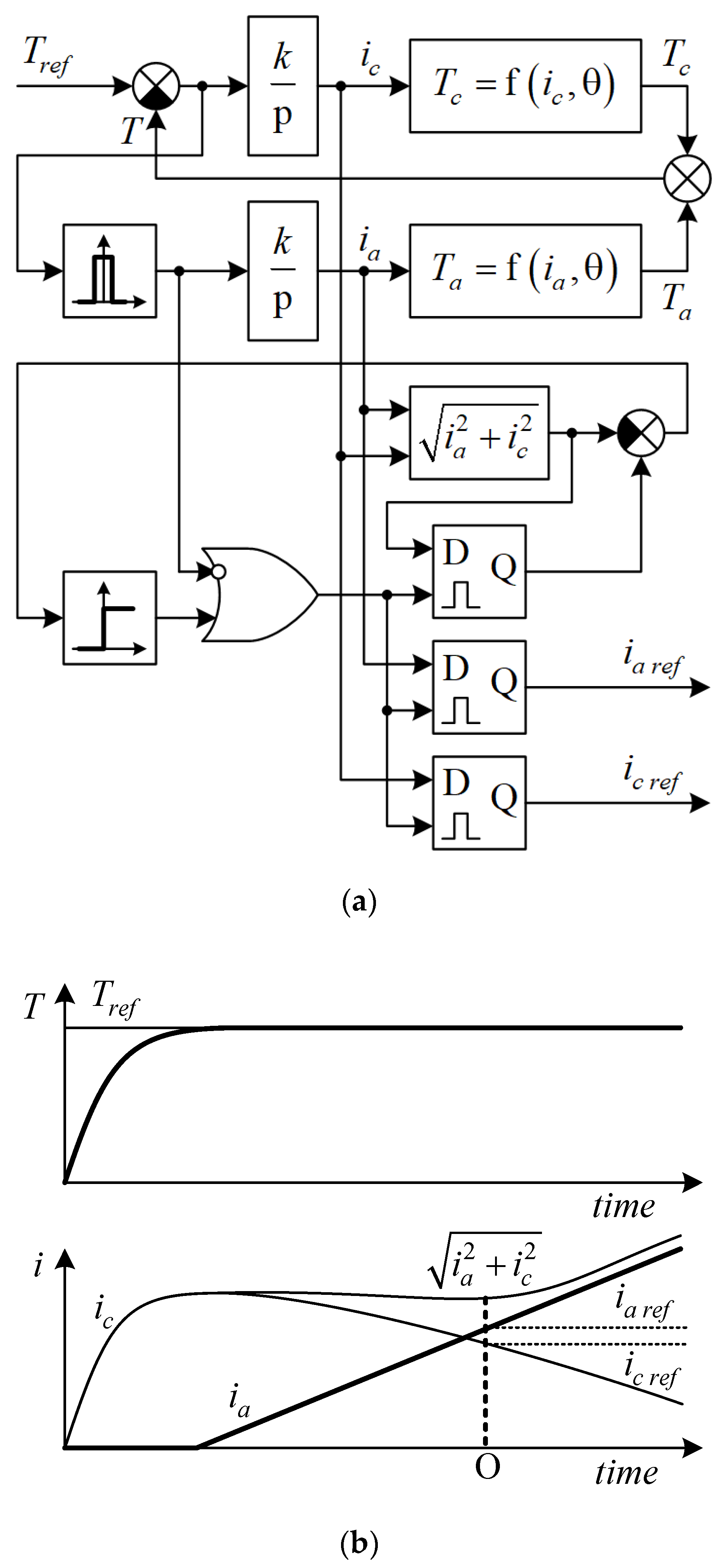
Consider some small positive angle (point O in Figure 3a) where the positive torque can be produced by phases A and C. Set the initial phase A and C currents to zero. The phase C current can be adjusted by integral torque controller, which has some gain k as shown in Figure 5a. The integral torque controller regulates the phase C current until the error in the torque reaches the permitted tolerance. Thereafter, the phase A current starts to increase (see Figure 5b). The torque controller maintains its operation, continuously time varying the phase C current and keeping the total torque from both phases A and C close to the reference.

From the moment when the phase A current starts to grow, the system begins to track the minimum total current as it determines the ohmic losses in the motor windings. In the end of the transient from Figure 5b, the outputs hold the most efficient references of the phase currents i_{a ref} and i_{c ref}, which can be used as points on the current reference surfaces for each phase as shown in Figure 3b.

A similar approach can be used for the angles when the positive torque is generated by one phase only. The only difference is that the search for minimal loss points is no longer needed due to the fact that total torque is produced by a single phase, and there is no extra degree of freedom.

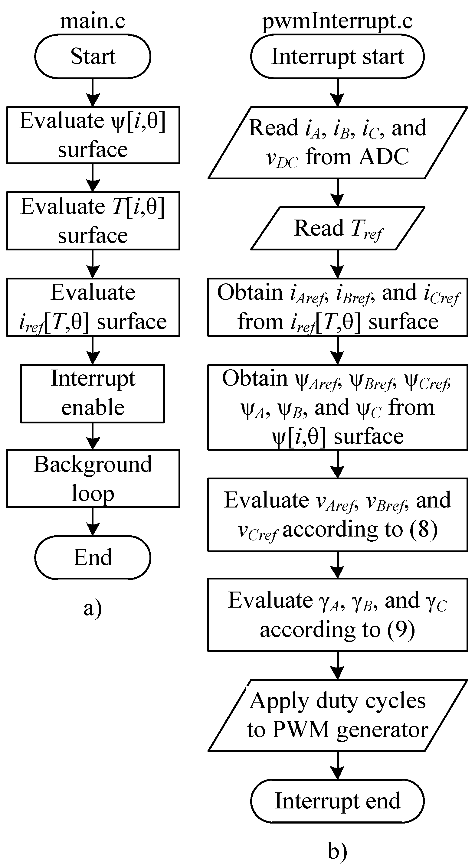
4.3. Control System Flowchart

The control system is divided into an offline time-consuming algorithm placed into the initialization stage, as shown in Figure 6a, and a real-time control interrupt (see Figure 6b), which implements the proposed model predictive control strategy.

First, for the given representation of the magnetization surface, the initialization procedure evaluates the flux linkage surface for the desired resolution of the two-dimensional array, for example, 100∙100 points. Next, these data are used to evaluate the torque surface using Equation (12). Finally, the most time-consuming algorithm is executed, which evaluates current references with respect to the range of all possible torque commands and angles using the iterative algorithm shown in Figure 5. Thereafter, the control system can start operation and rotate the machine.

The interrupt routine, which is shown in Figure 6b, should be executed at the end of the PWM cycle. The control system reads the feedback from the current, voltage, and position sensors inside this interrupt. At first, it uses the current reference surface to obtain current references for the next computed rotor angular position using Equation (5). Then, it obtains flux linkages for the current and next referenced steps from the magnetization surface. Finally, the voltage command and the duty cycles are evaluated and applied as the references to the PWM generator just before the new PWM cycle starts.

5. Simulation Results

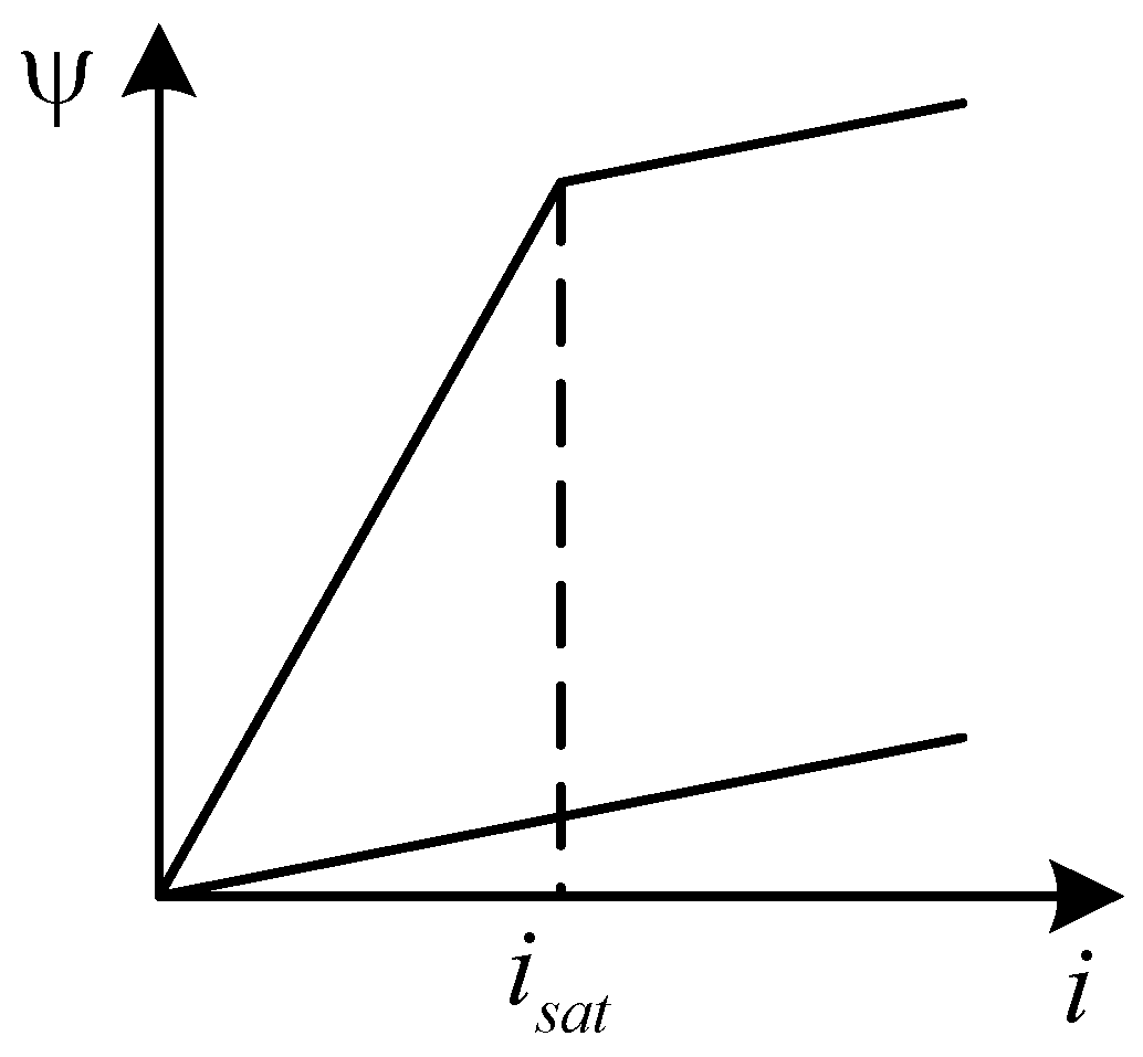
There are various approaches to building a model of SRM. One of the most convenient options is to use a linearized magnetization profile [16], as shown in Figure 7, which allows fast simulation with simple equations for torque estimation to be undertaken. Phase inductance below the saturation knee was found from the following equation:

$$L=L_{av}-\Delta L\cos \mathsf{\theta },$$

(13)

where $L_{av}$ is the average inductance, $\Delta L$ is the half-sum of maximum and minimum inductances, and $\mathsf{\theta }$ is the rotor electrical angular position. When operating above saturation current i_sat the phase differential inductance becomes equal to the minimal inductance of the motor for a misaligned position as assumed in Figure 7.

The Euler integration method was used to obtain flux linkage in each phase and the resulting equation is given below:

$$\mathsf{\psi }\left[m\right]=\mathsf{\psi }\left[m-1\right]+\left(v-iR\right)h,$$

(14)

where $\mathsf{\psi }\left[m\right]$ and $\mathsf{\psi }\left[m-1\right]$ are the new and previous flux linkages of the motor model, respectively, and h is the integration step size.

The power converter, which contains an asymmetrical H-bridge, is depicted in Figure 1. It can only produce a positive current in any phase, which should be taken into account in the model when zero or negative voltage is applied to the winding. If the numerically integrated flux linkage value in the model becomes negative, then it should be set to zero:

$$\mathsf{\psi }\left[m\right]=\{\begin{array}{l}\mathsf{\psi }\left[m\right],\hspace{0.17em}\mathsf{\psi }\left[m\right]\ge 0;\\ 0,\hspace{0.17em}\mathsf{\psi }\left[m\right]<0.\end{array}$$

(15)

The value of the current in the phase winding was calculated in accordance with the estimated flux linkage and the inductance value found from Equation (13):

$$i=\frac{\mathsf{\psi }}{L}.$$

(16)

If the evaluated current lies above the saturation knee, which can be checked by comparing it with the saturation current, then Equation (13) is not applicable and the phase current should be evaluated taking into account the differential inductance of the phase using the following equation:

$$i=i_{sat}+\frac{\mathsf{\psi }-L\cdot i_{sat}}{L_{min}}$$

(17)

instead of Equation (16), where $L_{min}$ is the minimum or differential inductance of the winding. If the actual current is smaller than the saturation current value, then the torque of a single phase was calculated using:

$$T=\frac{i^2}{2}\frac{\mathrm{d}L\left(\mathsf{\theta }\right)}{\mathrm{d}\mathsf{\theta }}=\frac{i^2}{2}\frac{\mathrm{d}\left(L_{av}-\Delta L\cos \mathsf{\theta }\right)}{\mathrm{d}\mathsf{\theta }}=\frac{\Delta L}{2}{i}^2\sin \mathsf{\theta }.$$

(18)

The torque in the operation point above the saturation knee, in addition, was evaluated using co-energy, which can be expressed as:

$${\mathrm{W}}^{\prime }\left(i,\mathsf{\theta }\right)=\left(L_{av}-\Delta L\cos \mathsf{\theta }\right)\left(\frac{i_{sat}^2}{2}+i_{sat}\left(i-i_{sat}\right)\right)+L_{min}{i}_{sat}\left(i-i_{sat}\right).$$

(19)

Then torque was found using:

$$T={\frac{\partial {\mathrm{W}}^{\prime }\left(i,\mathsf{\theta }\right)}{\partial \mathsf{\theta }}|}_i=\left(i_{sat}i-\frac{i_{sat}^2}{2}\right)\Delta L\sin \mathsf{\theta }.$$

(20)

In this research, simulation was performed using C++ Builder. This tool was utilized in order to produce code for a control system suitable for further implementation using a microcontroller. The simulation was performed with the integration step size equal to 0.1 us. The parameters of the drive are listed in

Table 1. Switched reluctance drive (SRD) parameters.

Parameter	Value	Units
Minimal inductance	10.0	mH
Maximum inductance	100.0	mH
Saturation current	20	A
Phase resistance	0.05	Ohm
Pole pairs	4	-
Maximum phase current limit	100	A
DC link voltage	600	V
PWM frequency	2.0	kHz

. As the control strategy contains only lookup table operation, it was supposed that the computation time is close to zero and that it is possible to evaluate the voltage commands for the next PWM cycle immediately at the end of the current PWM period.

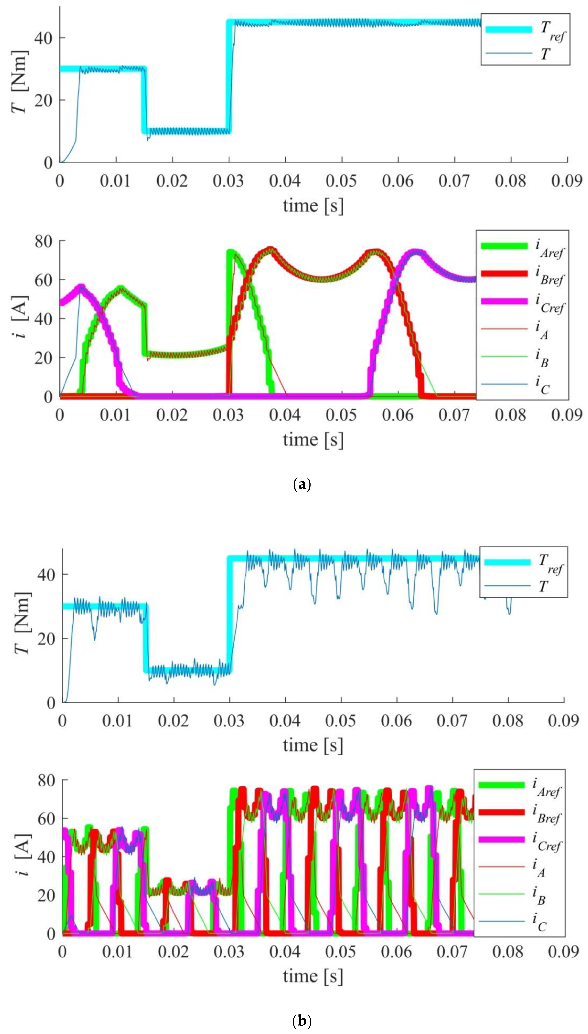
The motor was running at 80 rad/s. The torque reference was changed during simulation as shown in Figure 8a. Initially it was set to 30 Nm, then after 30 PWM cycles it was set to 10 Nm, and finally to 45 Nm after 60 PWM cycles. The torque response transient time was strongly dependent on the current inductance of the winding. For example, at the beginning of the simulation, the torque slope was limited by the high unsaturated inductance of phase C. As the current reached the saturation knee, the torque on the shaft started to grow more quickly. Then, inside the saturated region, the phase currents and output torque were regulated more rapidly. At the end of commutation cycle of the phase, the current reference varied faster than the minimum possible current slope due to the voltage limit.

The torque stabilization is sufficiently precise over the entire range of the loads. It has visible deviations due to the PWM nature of the inverter, which can be minimized by increasing the PWM frequency. The same load profile was applied to the motor operating at a higher speed equal to 480 rad/s (see Figure 8b). With the growth of the electrical speed, the voltage limit made stabilization of the commanded current impossible. Therefore, torque pulsation appears. This behavior is natural for switched reluctance drives [17,18] and can be slightly improved by adjusting the current reference profile with respect to the voltage limit.

6. Conclusions

Although the problem of precise torque control in switched reluctance motor drives was partially solved by means of finite control set model predictive control, the drive still suffers from an unpredictable switching rate and acoustic noise. The proposed solution implements a continuous control set MPC controlling power converter using pulse-width modulation and requires small computation efforts. It operates utilizing the assumption that optimal current reference profiles for each torque reference and angular position can be evaluated offline from the magnetization surface of the electrical machine. By knowing the current reference and magnetization surface, the voltage commands for the PWM-driven inverter can be evaluated using simple lookup tables, which has the advantage of practically zero computation delay and allows the calculation of the control law immediately at the end of each PWM cycle before applying the new duty cycles for the next PWM period.

The proposed CCS MPC can be implemented using modern microcontrollers. It was verified by a simulation model where accurate torque stabilization was achieved from zero to the rated speed. The settling time was limited by the supply voltage and the phase inductance.

Future work will be devoted to the practical implementation and verification of the proposed control strategy. In addition, it will address several questions that arose during this research.

Due to the current and torque slope limit when operating below the saturation knee, the proposed current reference profile is not optimal in terms of settling time. Nonetheless, it provides good efficiency of the motor and drive. Similar optimization of the current reference profiles is possible for operation at high speeds considering the voltage limit.

The sensitivity of the method to the inaccuracies of the model should be investigated, as well as the ability to use the current tracking error for identification of the rotor angular position for encoderless control.

References

- Rassolkin, A.; Kallaste, A.; Vaimann, T.; Tiismus, H. Control Challenges of 3D Printed Switched Reluctance Motor. In Proceedings of the 2019 26th International Workshop on Electric Drives: Improvement in Efficiency of Electric Drives (IWED), Moscow, Russia, 30 January–2 February 2019. [Google Scholar]
- Andrada, P.; Blanqué, B.; Martínez, E.; Perat, J.I.; Sánchez, J.A.; Torrent, M. Design of a Novel Modular Axial-Flux Double Rotor Switched Reluctance Drive. Energies 2020, 13, 1161. [Google Scholar] [CrossRef]
- Mademlis, C.; Kioskeridis, I. Performance Optimization in Switched Reluctance Motor Drives With Online Commutation Angle Control. IEEE Trans. Energy Convers. 2003, 18, 448–457. [Google Scholar] [CrossRef]
- Yu, C.; Xiao, Z.; Huang, Y.; Zhu, Y. Two-step commutation control of switched reluctance motor based on PWM. J. Eng. 2019, 2019, 8414–8418. [Google Scholar] [CrossRef]
- Zhang, M.; Bahri, I.; Mininger, X.; Vlad, C.; Xie, H.; Berthelot, E. A New Control Method for Vibration and Noise Suppression in Switched Reluctance Machines. Energies 2019, 12, 1554. [Google Scholar] [CrossRef]
- Huang, L.; Zhu, Z.Q.; Feng, J.H.; Guo, S.Y.; Li, Y.F.; Shi, J. Novel Current Profile of Switched Reluctance Machines for Torque Density Enhancement in Low-Speed Applications. IEEE Trans. Ind. Electron. 2019, 46, 1–11. [Google Scholar] [CrossRef]
- Ye, J.; Bilgin, B.; Emadi, A. An Offline Torque Sharing Function for Torque Ripple Reduction in Switched Reluctance Motor Drives. IEEE Trans. Energy Convers. 2015, 30, 726–735. [Google Scholar] [CrossRef]
- Lukman, G.F.; Nguyen, X.S.; Ahn, J.-W. Design of a Low Torque Ripple Three-Phase SRM for Automotive Shift-by-Wire Actuator. Energies 2020, 13, 2329. [Google Scholar] [CrossRef]
- Inderka, R.B.; Doncker, R.W.A.A. De DITC—Direct Instantaneous Torque Control of Switched Reluctance Drives. IEEE Trans. Ind. Appl. 2003, 39, 1046–1051. [Google Scholar] [CrossRef]
- Krishnan, R. Switched Reluctance Motor Drives Modeling, Simulation, Analysis, Design, and Applications, 1st ed.; CRC Press: Boca Raton, FL, USA, 2001; ISBN 0849308380. [Google Scholar]
- Parreira, B.; Rafael, S.; Pires, A.J.; Branco, P.J.C. Obtaining the magnetic characteristics of an 8/6-switched reluctance machine: FEM analysis and experimental tests. IEEE Trans. Ind. Electron. 2005, 52, 1635–1643. [Google Scholar] [CrossRef]
- Ramanarayanan, V.; Venkatesha, L.; Panda, D. Flux-linkage characteristics of switched reluctance motor. In Proceedings of the International Conference on Power Electronics, Drives and Energy Systems for Industrial Growth, New Delhi, India, 8–11 January 1996; Volume 1, pp. 281–285. [Google Scholar]
- Lin, Z.; Reay, D.S.; Zhou, B. Experimental measurement of Switched Reluctance Motor non-linear characteristics. In Proceedings of the IECON 2013—39th Annual Conference of the IEEE Industrial Electronics Society, Vienna, Austria, 10–13 November 2013; pp. 2827–2832. [Google Scholar]
- Anuchin, A.; Grishchuk, D.; Zharkov, A.; Prudnikova, Y.; Gosteva, L. Real-time model of switched reluctance drive for educational purposes. In Proceedings of the 2016 57th International Scientific Conference on Power and Electrical Engineering of Riga Technical University (RTUCON), Riga, Latvia, 13–14 October 2016. [Google Scholar]
- Cossar, C.; Popescu, M.; Miller, T.; McGilp, M. On-line phase measurements in switched reluctance motor drives. In Proceedings of the 2007 European Conference on Power Electronics and Applications, Aalborg, Denmark, 2–5 September 2007; pp. 1–8. [Google Scholar]
- Li, C.; Wang, G.; Liu, J.; Li, Y.; Fan, Y. A Novel Method for Modeling the Electromagnetic Characteristics of Switched Reluctance Motors. Appl. Sci. 2018, 8, 537. [Google Scholar]
- Ding, W.; Liu, G.; Li, P. A hybrid control strategy of hybrid-excitation switched reluctance motor for torque ripple reduction and constant power extension. IEEE Trans. Ind. Electron. 2020, 67, 38–48. [Google Scholar] [CrossRef]
- Rekik, M.; Besbes, M.; Marchand, C.; Multon, B.; Loudot, S.; Lhotellier, D. Improvement in the field-weakening performance of switched reluctance machine with continuous mode. IET Electr. Power Appl. 2007, 1, 785–792. [Google Scholar] [CrossRef]
© 2020 by the authors. Licensee MDPI, Basel, Switzerland. This article is an open access article distributed under the terms and conditions of the Creative Commons Attribution (CC BY) license (http://creativecommons.org/licenses/by/4.0/).