Article

Circuit Model and Analysis of Multi-Load Wireless Power Transfer System Based on Parity-Time Symmetry

School of Electric Power Engineering, South China University of Technology, Guangzhou 510641, China
*
Author to whom correspondence should be addressed.
Energies 2020, 13(12), 3260; https://doi.org/10.3390/en13123260
Submission received: 1 June 2020 / Revised: 21 June 2020 / Accepted: 22 June 2020 / Published: 24 June 2020
(This article belongs to the Section F: Electrical Engineering)

Abstract

:
In the multi-load wireless power transfer (WPT) system, the output power and transfer efficiency will drop significantly with the change of distance between transmitter and receiver. Power distribution among multiple loads is also a major challenge. In order to solve these problems, a novel multi-load WPT system based on parity–time symmetry (PT-WPT) is proposed in this paper. Firstly, the multi-load PT-WPT system is modeled based on the circuit model. Then, the transmission characteristics of the multi-load PT-WPT system are analyzed. It is found that constant output power with constant transfer efficiency can be maintained against the variation of coupling coefficient, and the power distribution relationship among loads is only related to the coupling coefficient. Further, power distribution under different coupling situations is analyzed in detail to meet different power demands. Finally, taking a dual-load PT-WPT system as an example, the system parameters are designed and the circuit simulation is carried out. The simulation results are consistent with the theoretical analysis, which shows that PT symmetry can be applied to the multi-load WPT system to achieve constant output power, constant transfer efficiency, and power distribution simultaneously.

Graphical Abstract

1. Introduction

Wireless power transfer (WPT) is a kind of technology that does not need wires or other physical connection and transmits electricity through the air. It has the advantages of flexible power supply and no cable constraints. In recent years, WPT technology has been widely used in portable electronic equipment, smart homes, electric vehicles, rail transit, implantable medical power supplies, or other fields. In the future, WPT technology will have broad application prospects in energy anomaly consumption detection [1,2], simultaneous wireless information and power transfer (SWIPT) [3,4], and so forth. However, the common wireless charging products on the market are mostly based on a single load at present. With the increasing number of electronic products with wireless power receiving function, the single-load WPT system cannot meet the demand of wireless power supply for multiple devices at the same time.
Therefore, the multi-load WPT system has become one of the research hotspots of wireless power transfer technology. Generally, most of the existing multi-load WPT systems are inductively coupling systems, magnetic resonant coupling systems, or microwave transmission systems, whose output power as well as the transfer efficiency is sensitive to the change of the coupling coefficient. So, there are some key technologies in the design of the multi-load WPT system.
One of the most important technologies is the stable output power and stable transfer efficiency. In practical applications, the distance between transmitter and receivers always varies with the operation status, which makes the output power and transfer efficiency unsteady and very sensitive to the load position. A large transmitting coil plane is a simple method to improve the output stability of the system, including single coil [5,6], coil array [7,8], and the repeater coils [9], by increasing the magnetic field area. But the steady output can only be achieved within the range of the transmitting plane, so the spatial freedom is very low. In order to improve the spatial freedom, omnidirectional multi-load WPT systems have been put forward; 2D and 3D WPT systems were proposed to realize omnidirectional wireless charging with two or three orthogonal coils by Lin et al. [10,11], Su et al. [12], and Han et al. [13]. These systems can maintain a constant output if the loads rotate around the transmitter at a constant radius. However, due to the uneven magnetic field, the output is unstable if the rotating radius changes. Liu et al. [14] proposed a multi-load WPT system based on a rotary transmitting coil which was driven by an electric motor. This method is simple to control, but the use of a motor increases the cost and volume of the system, resulting in low practicality. Moreover, a wireless charging box based on a square Helmholtz coil was developed by Zhang et al. [15], which could provide continuous wireless power to multiple mobile phones simultaneously even when they were moving. However, the efficiency changes significantly when the angle between the receiving coil and the magnetic field changes. A cavity resonator (CR) or quasistatic cavity resonance (QSCR) WPT system using the electromagnetic resonant modes of a hollow metallic structure has been proposed by Chabalko et al. [16,17]. This technique successfully transfers power wirelessly to multiple receivers contained anywhere within the chamber. However, the magnetic field distribution in the metal cavity is not uniform enough, so the output power and efficiency will change with the load position.
Another important technology is the power distribution among multiple loads, because different loads have different power demands. The current commonly used power distribution methods include: impedance matching method [18,19], time-sharing control method [20], frequency-division control method [21], hierarchical power control algorithm [22], adding DC/DC converter on the receiver [23], and so forth. In the above methods, either additional control circuits need to be added, or the control algorithm is too complicated. Therefore, it is urgent to propose a multi-load WPT system which can not only achieve constant output power and constant transfer efficiency of the system, but also realize power distribution simply and efficiently.
Parity–time (PT) symmetry is a kind of physical theory which is widely used in quantum mechanics and optics [24,25]. Further, it has been gradually applied to electricity by Schindler et al. [26] and Lin et al. [27]. Assawaworrarit et al. [28] first applied PT symmetry to the WPT system. The PT-symmetric WPT (PT-WPT) system achieves constant output power and constant efficiency within a distance of 1 m between transmitter and receiver. However, due to the use of an operational amplifier, the output power is very low (only milliwatts), and the overall system is also very inefficient (less than 10%). So, Zhou et al. [29] proposed an improved nonlinear saturated gain PT-WPT system constructed by a self-oscillating controlled inverter, which makes the output power reach hundreds of watts. Despite its many advantages, the PT symmetry has not been applied to the multi-load WPT system. So, it is valuable to expand the PT symmetry in multi-load WPT systems.
The main contribution of this paper is to model and analyze the multi-load WPT system based on the parity–time symmetry, which expands the single-load PT-WPT system to a multi-load system. Furthermore, this paper analyzes the PT symmetry conditions, transmission characteristics, and power distribution relationship between loads of the multi-load PT-WPT system using the circuit theory.
The remainder of this paper is organized as follows. Section 2 establishes the circuit model of the multi-load PT-WPT system using the circuit model theory. Then, Section 3 analyzes the transmission characteristics of the multi-load PT-WPT system. Section 4 introduces the power distribution between loads under different coupling situations. Section 5 designs the parameters of a dual-load PT-WPT system and presents the circuit simulation results. Finally, some conclusions are given in Section 6.

2. Modeling of Multi-Load PT-WPT System

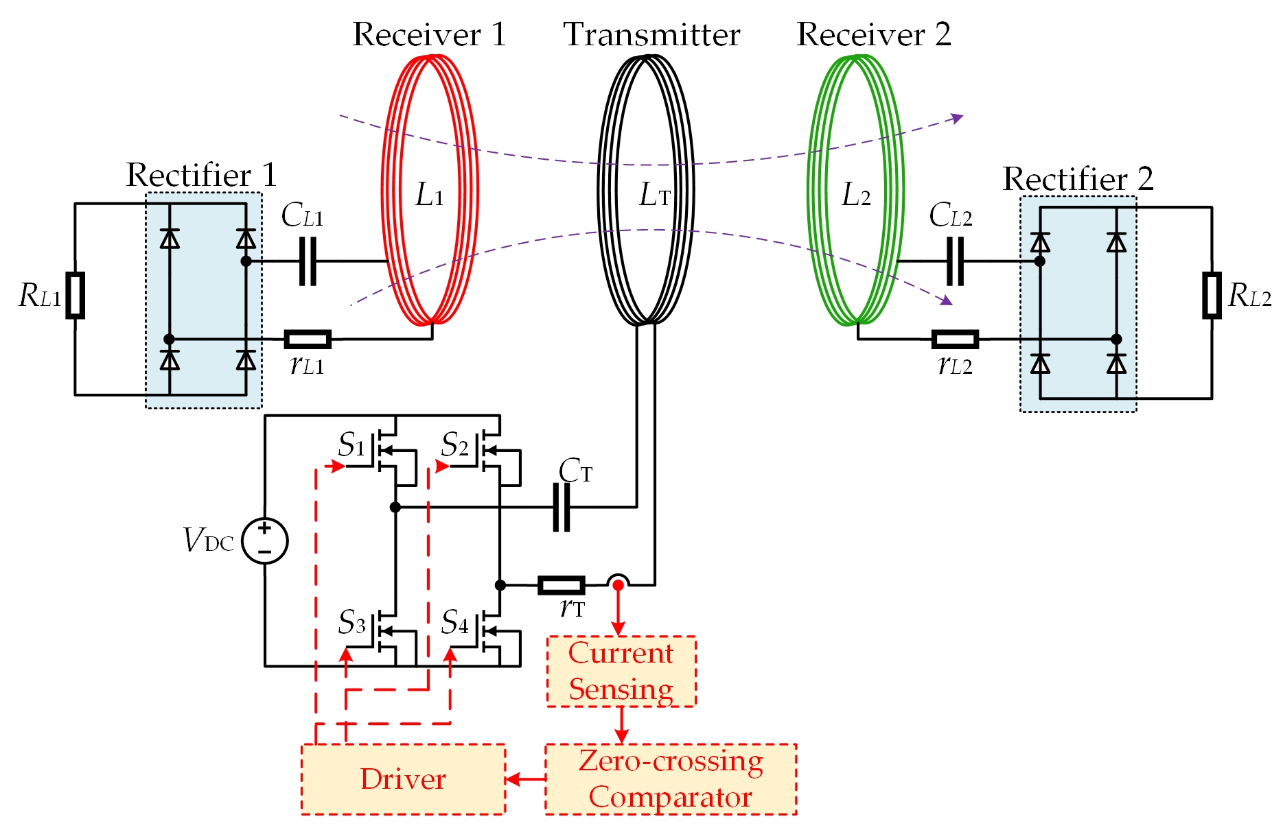
2.1. PT Principle in WPT System with Operational Amplifier

The so-called PT-symmetric systems are invariant under the joint parity and time reversal operation [28,30]. The nonlinear PT-symmetric model is realized by a parallel–parallel topology of the WPT system [28]. Indeed, both the series–series topology and the parallel–parallel topology of the WPT system can be used to realize the nonlinear PT-symmetric model [29]. The structure of the single-load PT-WPT system is shown in Figure 1a, including the gain unit and the loss unit, in which the gain unit is composed of an operational amplifier, R1, Rf1, and Rf2. LT and CT are coil inductance and resonant capacitor on the transmitter, respectively; LR and CR are coil inductance and resonant capacitor on the receiver, respectively; iT and iR are currents flowing through the transmitter and receiver, respectively; RL is the load resistance; and M is the mutual inductance.
Due to the operational amplifier’s saturation voltage, both ends of ab can be equivalent to a nonlinear negative resistance −RN with a resistance value of −R1/(A−1), wherein A = 1 + Rf1/Rf2 [28]. Therefore, the equivalent circuit is shown in Figure 1b. The negative resistance −RN will input power into the LC series resonant circuit at the transmitter, and then transmit the energy to the load through the magnetic coupling between the transmitting coil and the receiving coil.
Based on Kirchhoff’s voltage law, the circuit model of the single-load PT-WPT system as shown in Figure 1b can be fully described as follows:
[ R N + r T L T + j ω j ω T 2 ω j ω k L R L T j ω k L T L R R L + r R L R + j ω j ω R 2 ω ] × [ I ˙ T I ˙ R ] = 0
where I ˙ T and I ˙ R are current vectors of iT and iR, respectively; ω is the operating angle frequency of the system; ωT and ωR are the natural resonant angular frequencies of the transmitting side and receiving side, respectively, which are denoted as ω T = 1 / L T C T , ω R = 1 / L R C R ; rT and rR are the internal resistance; the coupling coefficient k is k = M / L T L R .
The PT-symmetric WPT system requires that ωT = ωR = ω0 [28]. Further, the determinant must be zero, then Equation (1) has a nonzero solution. Hence, taking ω to be real, separate the real and imaginary parts to obtain Equation (2) as follows.
{ ( R N + r T ) ( R L + r R ) L T L R ( ω ω 0 2 ω ) 2 + ω 2 k 2 = 0 ( ω ω 0 2 ω ) ( R N + r T L T + R L + r R L R ) = 0
According to Equation (2), it can be seen that (−RN + rT)/LT + (RL + rR)/LR = 0 must be satisfied, which is consistent with the requirement that the gain rate of the transmitter needs to be equal to the loss rate of the receiver [28]. So, the PT-symmetric conditions can be expressed as:
{ ω T = ω R = ω 0 R N + r T L T = ( R L + r R ) L R
There are two regions containing solutions of Equation (2), depending on the coupling coefficient k, as shown in Figure 2a, wherein k c = 1 1 4 × [ 2 ( R L + r R ω 0 L R ) 2 ] 2 is defined as the critical coupling coefficient. In the strong coupling region (kck < 1), the system supports two modes with angular frequencies, as shown in Equation (4). These two modes have the same saturated gain, exactly balancing out the loss. That means the energy stored in the transmitting and receiving resonators will remain equal. In addition, the operating angular frequency ω will be automatically adjusted with the change of k. In the weak coupling region (0 < k < kc), only one mode is located at ω = ω0, with the corresponding saturated gain less than the loss.
ω = ω 0 2 ( 1 k 2 ) × 2 ( R L + r R ω 0 L R ) 2 ± [ 2 ( R L + r R ω 0 L R ) 2 ] 2 + 4 ( k 2 1 )
Further, in the matched PT-symmetric conditions, the system output power and transfer efficiency can be obtained as follows:
P o = V o 2 R L = { R L V i n 2 L T ( R L + r R ) 2 L R + 2 ( R L + r R ) r T + L R L T r T 2 , k c k < 1 R L ( R L + r R L R ) 2 V i n 2 k 2 ω 0 2 ( L T ( R L + r R ) 2 L R + 2 ( R L + r R ) r T + L R L T r T 2 ) , 0 < k < k c
η o = I R 2 R L I T 2 r T + I R 2 r R + I R 2 R L = { R L L T r T L R + L T ( R L + r R ) , k c k < 1 R L L T r T ( R L + r R ) 2 k 2 ω 0 2 L R + L T ( R L + r R ) , 0 < k < k c
where Vo, Vin, IR, and IT are the effective value of vo, vin, iR, and iT, respectively. The system transmission characteristics are as shown in Figure 2b. In the strong coupling region, the output power and transfer efficiency are independent of k and only related to the inherent parameters. Hence the output power and transfer efficiency will remain constant against the variation of the coupling coefficient. However, in the weak coupling region, the output power and transfer efficiency fluctuate drastically due to the change of coupling coefficient k.

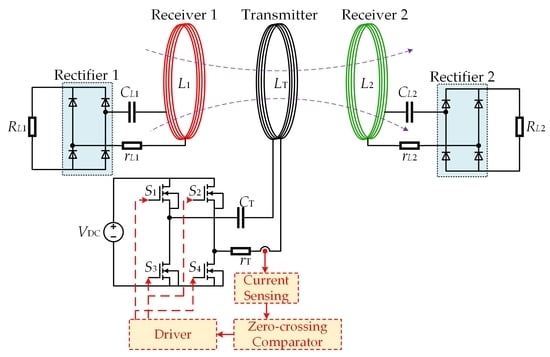
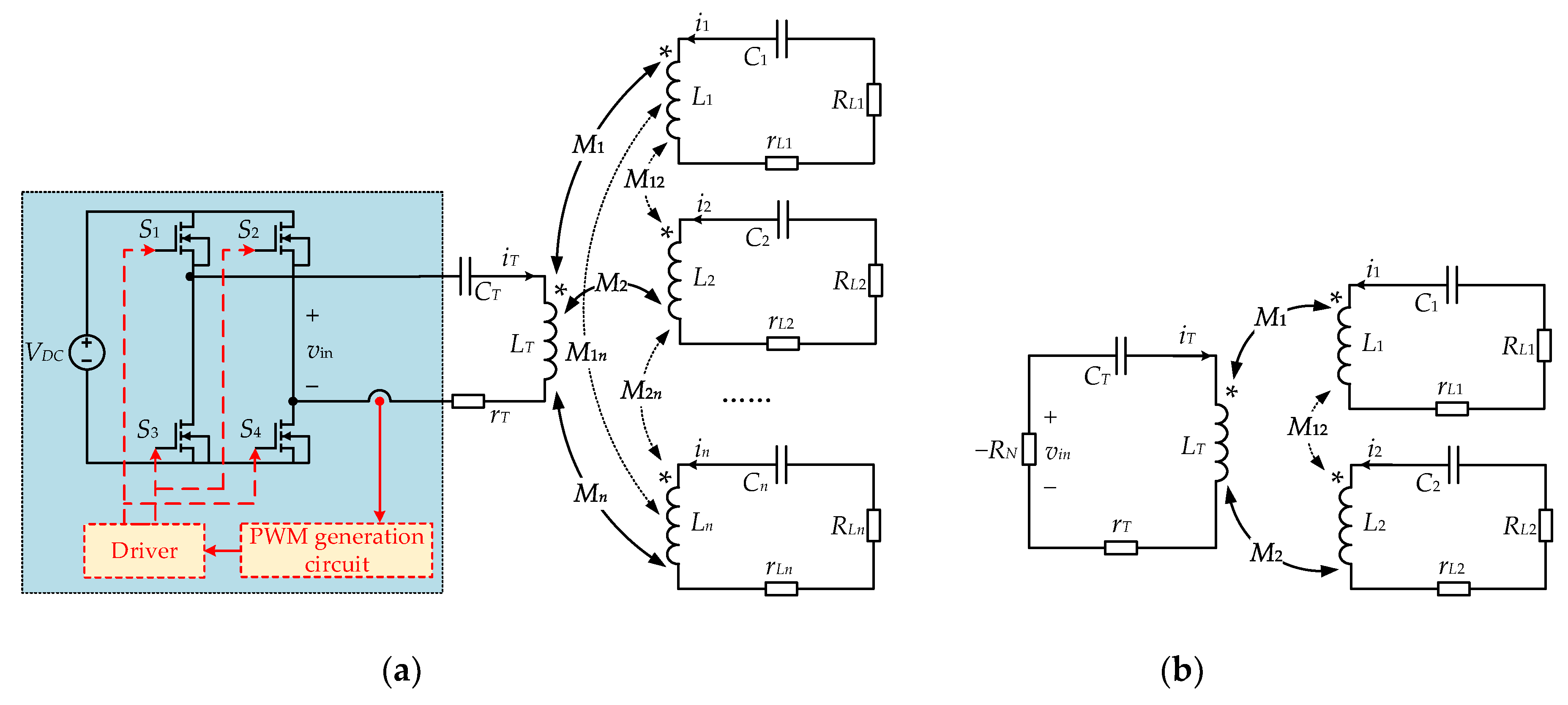
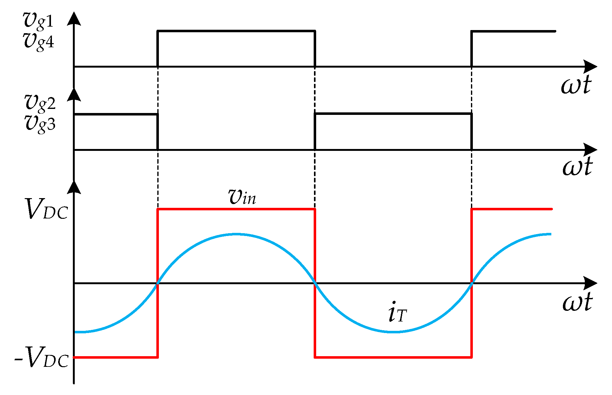
2.2. Circuit Model of Multi-Load PT-WPT System with Self-Oscillating Full-Bridge Inverter

According to Section 2.1, the PT-WPT system has obvious advantages in improving the system stability and spatial freedom, compared with the traditional resonant or inductive WPT system. But the existing research is only for single-load PT-WPT systems. Therefore, a multi-load PT-WPT system is proposed in this section, which is more suitable for wireless charging of multiple electrical appliances in practice.
A full-bridge inverter is used to construct a nonlinear saturation gain system in this paper instead of the operation amplifier to achieve higher output power. The circuit of PT-WPT system with n loads is shown in Figure 3a, wherein the full-bridge inverter is a self-oscillating controlled inverter; LT, CT, rT, and iT are coil inductance, resonant capacitor, internal resistance, and coil currents on the transmitter, respectively; Li, Ci, rLi, and ii are coil inductance, resonant capacitor, internal resistance, and coil current on the ith receiver, respectively; RLi is the ith load resistance; Mi is the mutual inductance and Mij is the cross-coupling mutual inductance between the transmitting coils (i, j = 1, 2, …, n).
Figure 4 shows the waveform of vin, as well as iT and the gate drive signal of S1, S2, S3, and S4 (vg1, vg2, vg3, and vg4). To simplify the analysis, the delay time and dead time are not considered in the modeling. As shown in Figure 4, the full-bridge inverter is controlled by zero crossing points of the current waveform in the transmitting resonator. So, vin can be defined as:
v i n = s g n ( i T ) × V D C
Assuming the direction of current iT and voltage vin shown in Figure 3 is positive, Figure 4 shows that the phase difference between vin and iT is 0°, which means generating energy. Therefore, the full-bridge inverter can also be equivalent to a negative resistance −RN, as shown in Figure 3b.
According to Kirchhoff’s voltage law, the circuit model of the multi-load PT-WPT system can be obtained, as presented in Equation (8).
[ R N + r T + j ω L T j 1 ω C T j ω M 1 j ω M n j ω M 1 R L 1 + r L 1 + j ω L 1 j 1 ω C 1 j ω M 1 n j ω M n j ω M 1 n R L n + r L n + j ω L n j 1 ω C n ] [ I ˙ T I ˙ 1 I ˙ n ] = 0
In order to initially explore the feasibility of the multi-load PT-WPT system and simplify the calculation, the circuit model of the PT-WPT system with two loads will be modeled and analyzed in detail. The equivalent circuit is shown in Figure 3b. When the receiving coils L1 and L2 are respectively located on both sides of the transmitting coil and are far away from each other, the cross-coupling between the two receiving coils has little effect on the system, which can be ignored approximately, that is, M12 = 0. According to Kirchhoff’s voltage law, the circuit model of the dual-load PT-WPT system can be obtained, as presented in Equation (9).
[ R N + r T L T + j ( ω ω T 2 ω ) j ω k 1 L 1 L T j ω k 2 L 2 L T j ω k 1 L T L 1 R L 1 + r L 1 L 1 + j ( ω ω 1 2 ω ) 0 j ω k 2 L T L 2 0 R L 2 + r L 2 L 2 + j ( ω ω 2 2 ω ) ] [ I ˙ T I ˙ 1 I ˙ 2 ] = 0
where ω 1 = 1 / L 1 C 1 and ω 2 = 1 / L 2 C 2 are the natural resonant angular frequencies of the two receivers, and the coupling coefficients k1 and k2 are defined as k 1 = M 1 / L T L 1 , k 2 = M 2 / L T L 2 .
A PT-symmetric system not only requires that the natural resonant frequencies of transmitter and receivers are the same (ωT = ω1 = ω2), but also requires that the structure and parameters of transmitter and receivers are symmetrical and equal, so Equation (10) must be satisfied as PT-symmetric conditions.
{ ω T = ω 1 = ω 2 = ω 0 R L 1 L 1 = R L 2 L 2 R N + r T L T = R L 1 + r L 1 L 1 = R L 2 + r L 2 L 2
Similarly, in order to have a nonzero solution, the determinant of Equation (9) must be zero. Furthermore, taking ω to be real, substitute Equation (10) into Equation (9) and separate the real and imaginary parts to obtain:
( k 1 2 + k 2 2 ) ω 4 ( ω 2 ω 0 2 ) 2 ( R L 1 + r L 1 L 1 ) 2 ω 2 = 0
and
[ ( k 1 2 + k 2 2 ) ω 4 ( ω 2 ω 0 2 ) 2 ( R L 1 + r L 1 L 1 ) 2 ] ( ω 2 ω 0 2 ) = 0

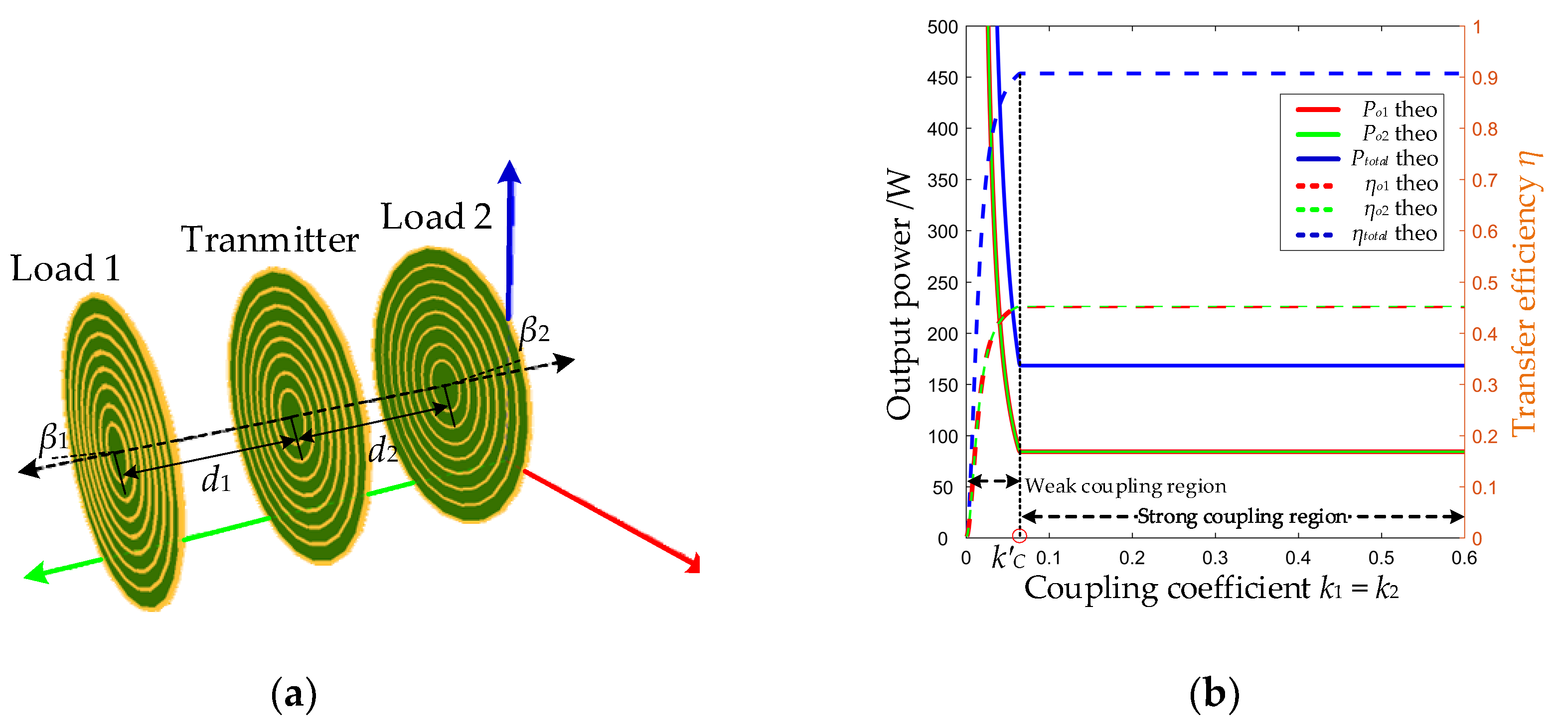
3. Analysis of the Transmission Characteristics of Multi-Load PT-WPT System

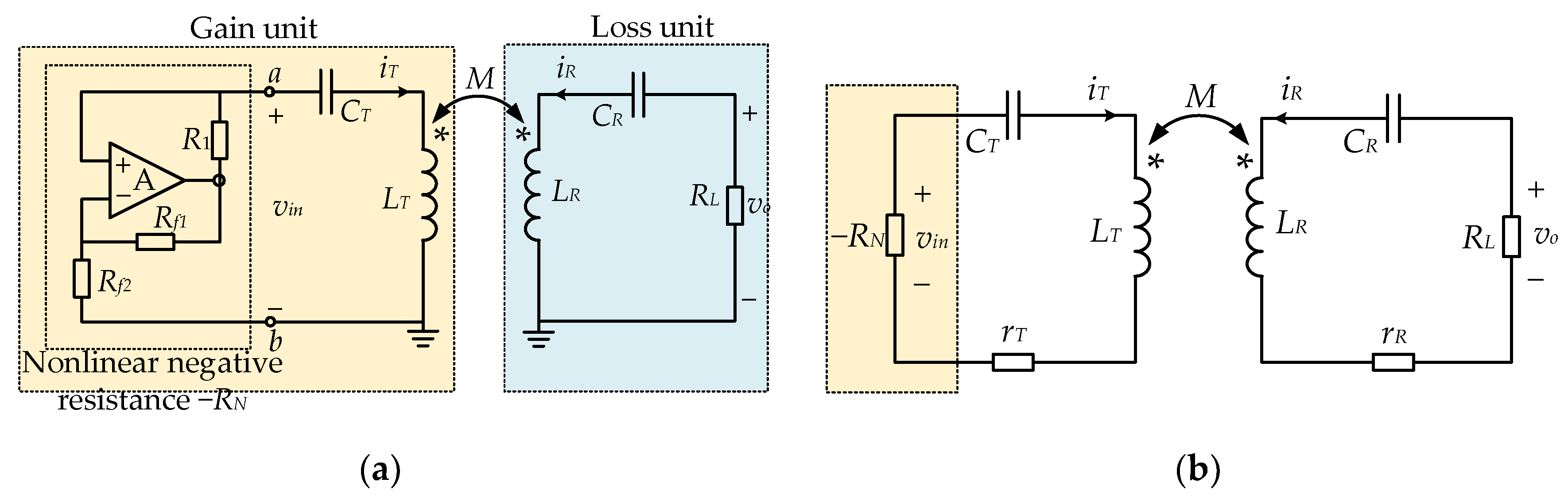
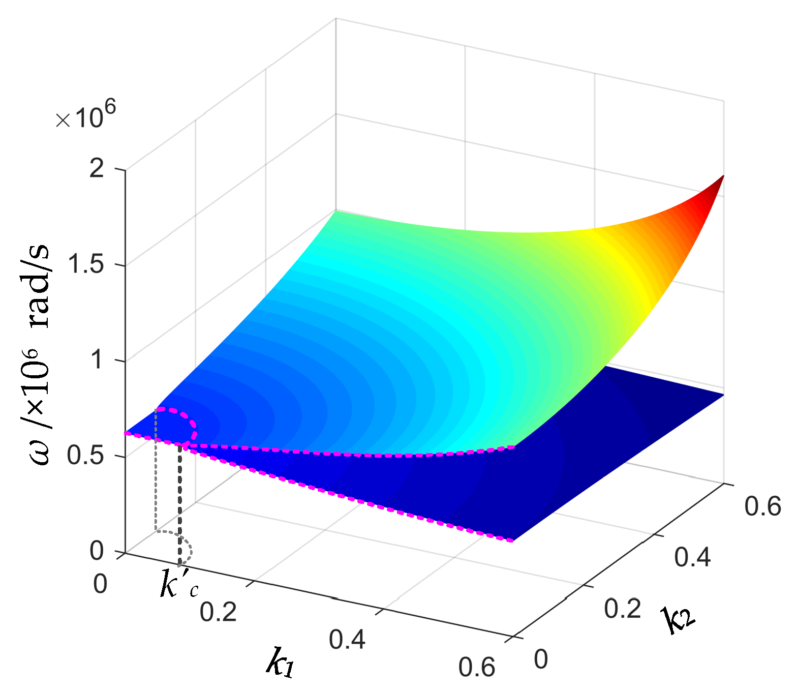
3.1. Operating Angular Frequency

From Equation (9) to (12), the angular frequency solution of the dual-load PT-WPT system can be derived as follows:
ω = { ω 0 2 [ 1 ( k 1 2 + k 2 2 ) ] 2 ( R L 1 + r L 1 ω 0 L 1 ) 2 ± [ 2 ( R L 1 + r L 1 ω 0 L 1 ) 2 ] 2 + 4 ( k 1 2 + k 2 2 1 ) , k c 2 k 1 2 + k 2 2 < 1 ω 0 , 0 < k 1 2 + k 2 2 < k c 2
where k c = 1 1 4 × [ 2 ( R L 1 + r L 1 ω 0 L 1 ) 2 ] 2 is defined as the critical coupling coefficient in the multi-load PT-WPT system.
Based on the above analysis, it can be found that there are also two regions containing solutions of Equation (13), depending on the coupling coefficients k1 and k2, as shown in Figure 5. In the strong region ( k c 2 k 1 2 + k 2 2 < 1 ), which is called the PT-symmetric phase, the system supports two modes with two solutions of angular frequency; the gain of the system is fully balanced with all the losses. It is worth noting that the system can only work at one frequency at any time, and the system automatically adjusts the angular frequency with the change of k1 and k2, due to the nonlinear saturation gain. In the weak coupling region ( 0 < k 1 2 + k 2 2 < k c 2 ), which is called the PT broken phase, only one mode is located at ω = ω0.

3.2. Output Power and Transfer Efficiency

Substituting Equations (10)–(13) into Equation (9), the effective value of coil currents iT, i1, i2 can be obtained. Then, the total output power Ptotal and transfer efficiency ηtotal in the strong coupling region or P’total and η’total in the weak coupling region, the ith load’s output power Poi, and transfer efficiency ηoi can be expressed as follows (i = 1, 2).
(1) strong coupling region
P o 1 = R L 1 V i n 2 k 1 2 k 1 2 + k 2 2 L T ( R L 1 + r L 1 ) 2 L 1 + 2 ( R L 1 + r L 1 ) r T + L 1 L T r T 2
P o 2 = R L 2 V i n 2 k 2 2 k 1 2 + k 2 2 L T ( R L 2 + r L 2 ) 2 L 2 + 2 ( R L 2 + r L 2 ) r T + L 2 L T r T 2
P t o t a l = P o 1 + P o 2 = R L 1 V i n 2 L T ( R L 1 + r L 1 ) 2 L 1 + 2 ( R L 1 + r L 1 ) r T + L 1 L T r T 2
η o 1 = k 1 2 k 1 2 + k 2 2 R L 1 L T r T L 1 + L T ( R L 1 + r L 1 )
η o 2 = k 2 2 k 1 2 + k 2 2 R L 2 L T r T L 2 + L T ( R L 2 + r L 2 )
η t o t a l = η o 1 + η o 2 = R L 1 L T r T L 1 + L T ( R L 1 + r L 1 )
(2) weak coupling region
P t o t a l = R L 1 ( R L 1 + r L 1 L 1 ) 2 V i n 2 ω 0 2 ( k 1 2 + k 2 2 ) ( L T ( R L 1 + r L 1 ) 2 L 1 + 2 ( R L 1 + r L 1 ) r T + L 1 L T r T 2 )
η t o t a l = R L 1 L 1 ( k 1 2 + k 2 2 ) r T ( R L 1 + r L 1 ) 2 ω 0 2 L T + L 1 ( R L 1 + r L 1 ) ( k 1 2 + k 2 2 )
Here, Vin is the effective value of input voltage vin. From Equations (14)–(19), it can be seen that the total output power and transfer efficiency remain constant in the strong coupling region, while the output power and transfer efficiency of each load vary with k1 and k2. On the contrary, the total output power and transfer efficiency change drastically in the weak coupling region as shown in Equations (20) and (21), which is affected by k1 and k2 simultaneously. However, it can be further found that when k1 and k2 satisfy a certain condition in the strong coupling region, the output power and transfer efficiency of each load can still remain constant. The specific situation will be analyzed in detail in Section 4.

3.3. Comparison with Single-Load PT-WPT System

Based on the above modeling and analysis of the single-load PT-WPT system and dual-load PT-WPT system, the comprehensive comparison between the two systems is shown in Table 1 when the system works in the strong coupling region. It can be found that the dual-load PT-WPT system needs to meet stricter PT symmetric conditions and coupling coefficient conditions. When the system is in PT-symmetric phase, the total output power and total transfer efficiency of the dual-load PT-WPT system remain constant, and the whole system exhibits exactly the same characteristics as the single-load PT-WPT system. On the other hand, the output power and transfer efficiency of each load are distributed unevenly and vary with the coupling coefficient. It is only when a certain coupling coefficient condition is satisfied that each load can maintain a constant output power and constant transfer efficiency.

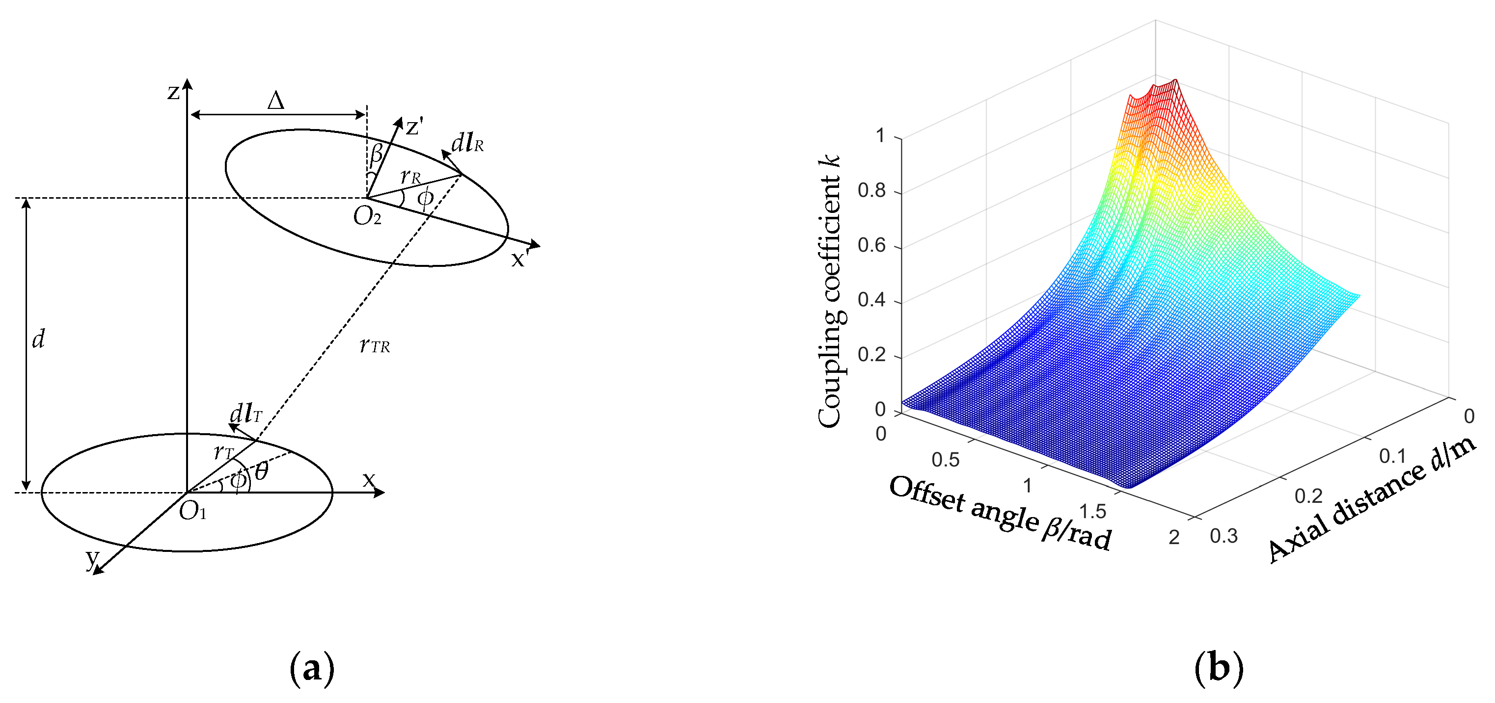
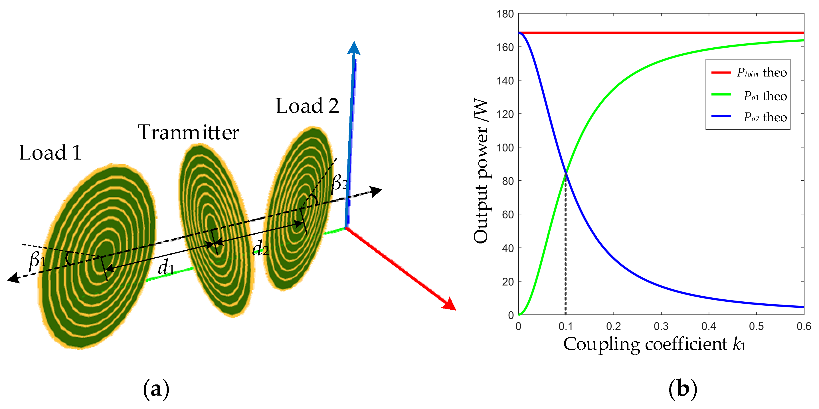
4. Power Distribution under Different Coupling Situations

According to the above analysis, the power and efficiency distribution of different loads in the strong coupling region can be obtained by
P o 1 P o 2 = k 1 2 k 2 2 ,   η o 1 η o 2 = k 1 2 k 2 2
Equation (22) shows that, for a dual-load PT-WPT system with known system parameters, the power and transfer efficiency of different loads only relate to the coupling coefficients k1 and k2. Therefore, before discussing the power distribution under different coupling situations, the relationship between the coupling coefficient and the coils’ position should be obtained first. The spatial arbitrary position of the two planar coils is shown in Figure 6a, where r′T and r′R are the radius of transmitting coil and receiving coil, respectively, d is the axial distance, Δ is the horizontal lateral shift distance between the centers of the two coils, and β is the offset angle between the normal directions. Further, the coupling coefficient k between two planar coils is a function of β, d, and Δ [31].
k ( β , d , Δ ) = N T N R μ 0 r T r R d ϕ sin θ sin ϕ cos β + cos θ cos ϕ r T R d θ 4 π L T L R
wherein
r T R = [ r T 2 + r R 2 + d 2 + Δ 2 + 2 Δ r R cos ϕ sin β 2 Δ r T cos θ 2 r R d cos ϕ sin β 2 r T r R ( cos θ cos ϕ cos β + sin θ sin ϕ ) ] 1 2
and NT, NR, LT, and LR are the coil turns and inductance of transmitting coil and receiving coil, respectively, μ0 is the magnetic permeability of vacuum. This paper mainly considers the influence of the relative position of the two planar coils on the proposed PT-WPT system, that is, Δ = 0, so the curve of the coupling coefficient with respect to the offset angle β and the coil center distance d is shown in Figure 6b.
Then, considering the variable loads position in practice, the power distribution can be divided into the following two cases according to the coupling situation.
(1) k1 = k2
In this case, Load 1 and Load 2 are symmetrically distributed on both sides of the transmitter, that is, β1 = β2 = β0, d1 = d2 = d0, as shown in Figure 7a. According to Equation (22), Po1 = Po2 = 50% Ptotal and ηo1 = ηo2 = 50% ηtotal can be obtained when k1 = k2. That means, in the strong coupling region, the total output power of the system is equally distributed to each load. According to the analysis in Section 3, the Ptotal and ηtotal of the dual-load PT-WPT system is always constant in the strong coupling region, so the output power and transfer efficiency of each load are also constant at any time and independent of the coupling coefficient, as long as k1 = k2 is always satisfied, as shown in Figure 7b.
In practice, using this characteristic, two loads with the same power demand can be wirelessly charged simultaneously. When the two loads move the same distance and offset angle at the same time to satisfy k1 = k2, the output power and transfer efficiency of each load remain constant. However, k1 and k2 shouldn’t be so small (k1 = k2 < k’c) that the system works in the weak coupling region, otherwise the output power of the system and each load will rise sharply and the transfer efficiency will drop sharply, as shown in Figure 7b, resulting in the system’s damage.
(2) k1k2
In this case, Load 1 and Load 2 are located on both sides of the transmitter arbitrarily. Suppose that Load 1 is first placed at a certain position (β1, d1) and Load 2 is placed at (β2, d2), as shown in Figure 8a. So, the coupling coefficients k1 and k2 can be calculated according to Equation (23) or by scanning Figure 6b. According to Equation (22), the output power of Load 1 and Load 2 can be obtained:
{ P o 1 = k 1 2 k 1 2 + k 2 2 P t o t a l P o 2 = k 2 2 k 1 2 + k 2 2 P t o t a l
It can be found that the output power of each load depends on k1 and k2. Users only need to adjust the coupling coefficient to achieve power distribution according to the power demands of different loads. However, in practice, the variation range of the coupling coefficient is not arbitrary. Once the difference between the two coupling coefficients is too large, the power distribution will be extremely uneven. The output power with too large coupling coefficient will be too large, which will easily damage the load. While the output power with a small coupling coefficient is too small, it cannot meet the load’s power demand. So, it is necessary to set the output power limit of each load. Suppose that the maximum allowable output power of Load 1 is Po1_max and the minimum output power is Po1_min. Therefore, the actual output power Po1 of Load 1 should satisfy Po1_max > Po1 > Po1_min. According to Equation (25), the variation range of k1 and k2 shall meet the following requirement.
P o 1 _ max P t o t a l P o 1 _ max k 1 k 2 P o 1 _ min P t o t a l P o 1 _ min
Further, according to the change of load position, there are two different situations in this case as follows. One situation is that one coupling coefficient changes while the other remains unchanged. The other situation is that two coupling coefficients k1 and k2 change simultaneously. Assume that the coupling coefficient k2 is fixed at k2 = 0.1, while k1 varies from 0.091 to 0.6 and k1k2 = 0.1. The power distribution between Load 1 and Load 2 is shown in Figure 8b. It can be seen that Load 1 and Load 2 cannot maintain a constant output power when k1 changes, while the total output power Ptotal of the system still remains constant. Although the position of Load 2 remains unchanged, its output power is still affected by k1. The power distribution between loads is uneven. Moreover, the larger the coupling coefficient is (that is, the receiving coil is closer to the transmitting coil), the larger the output power is.
In summary, the above two kinds of power distribution relationship of dual-load PT-WPT systems can provide reference for the further formulation of power distribution control strategy in the future. Combined with the relationship between coupling coefficient and load position shown in Figure 6, there are two methods to achieve constant output power and transfer efficiency of the system and each load simultaneously. One is to always satisfy k1 = k2, where the output power is evenly distributed to each load, that is Po1 = Po2 = 50% Ptotal and ηo1 = ηo2 = 50% ηtotal. The other is to design a control strategy that only adjusts the coupling coefficients automatically according to the power distribution relationship of k1k2 and the power demands of different loads, which does not need to add any compensation circuit.

5. System Parameter Design and Circuit Simulation Verification

5.1. System Structure and Parameter Design

To verify the results of the above theoretical analysis, a circuit simulation model is built. A full-bridge inverter is used to construct a nonlinear saturation gain system instead of half-bridge inverter as [29,32] to achieve higher output power. The schematic diagram of the simulation circuit of the dual-load PT-WPT system is shown in Figure 9. In addition, to show the wonderful characteristics of the actual dual-load PT-WPT system, the two receivers are coaxially located on both sides of the transmitter, and the two receiving coils are the same size as the transmitting coil, with a radius of 26 cm. The natural resonant frequency f0 of the transmitter and two receivers is set as 100 kHz. Moreover, in order to simulate the actual situation as much as possible, the parameters of the two loads are not exactly the same. The specific parameters are shown in Table 2.

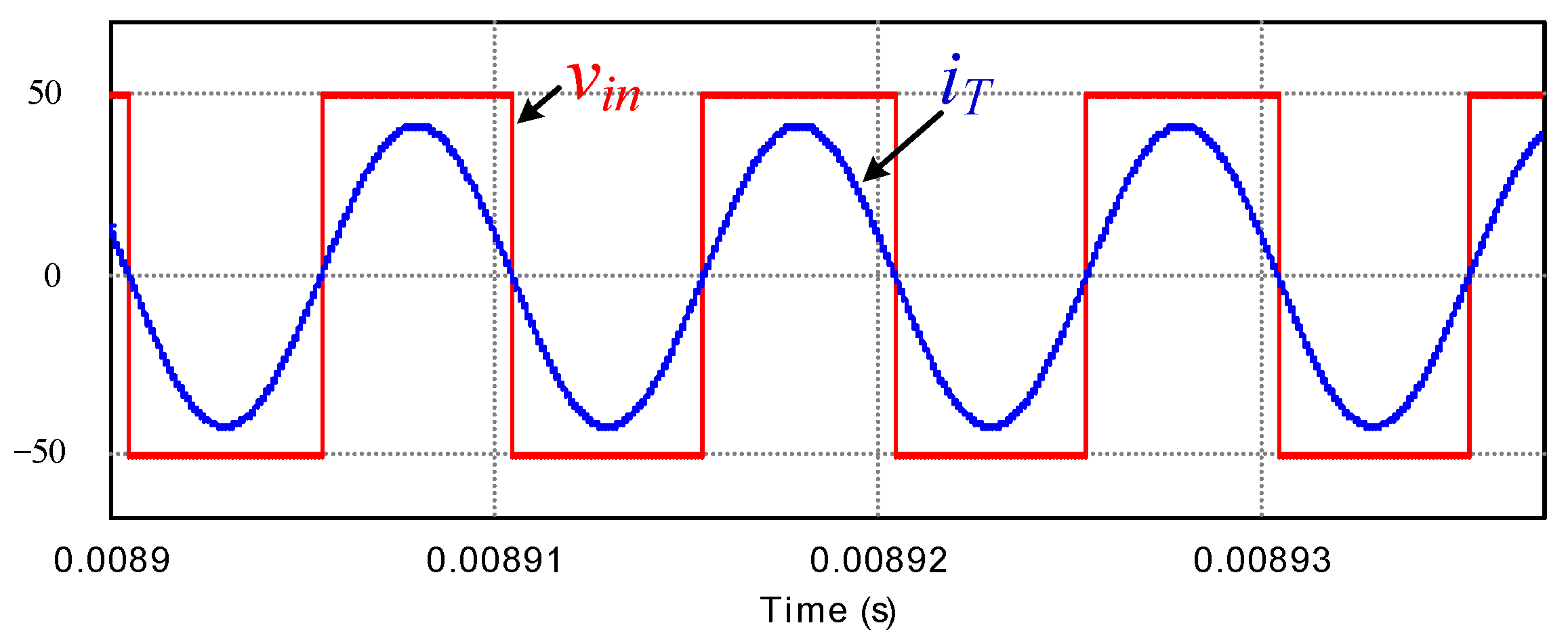
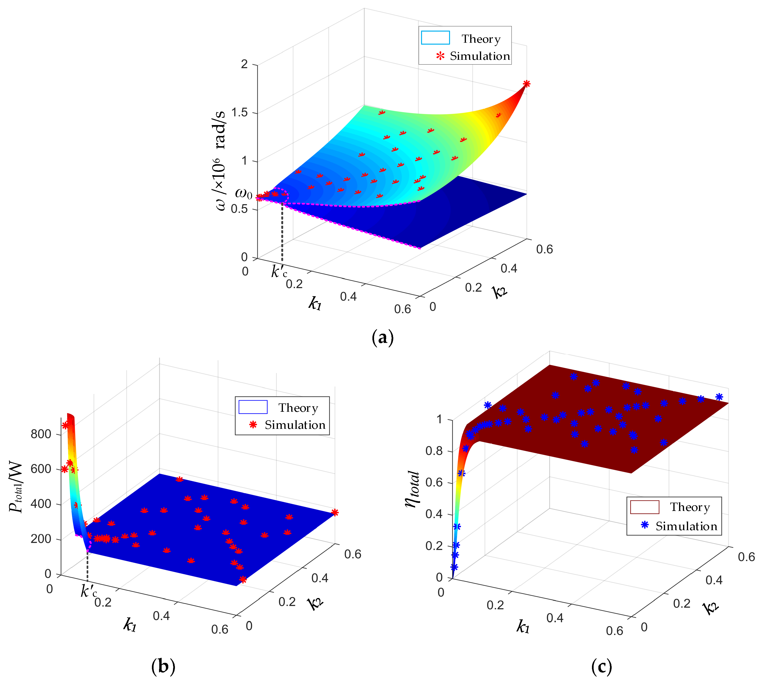
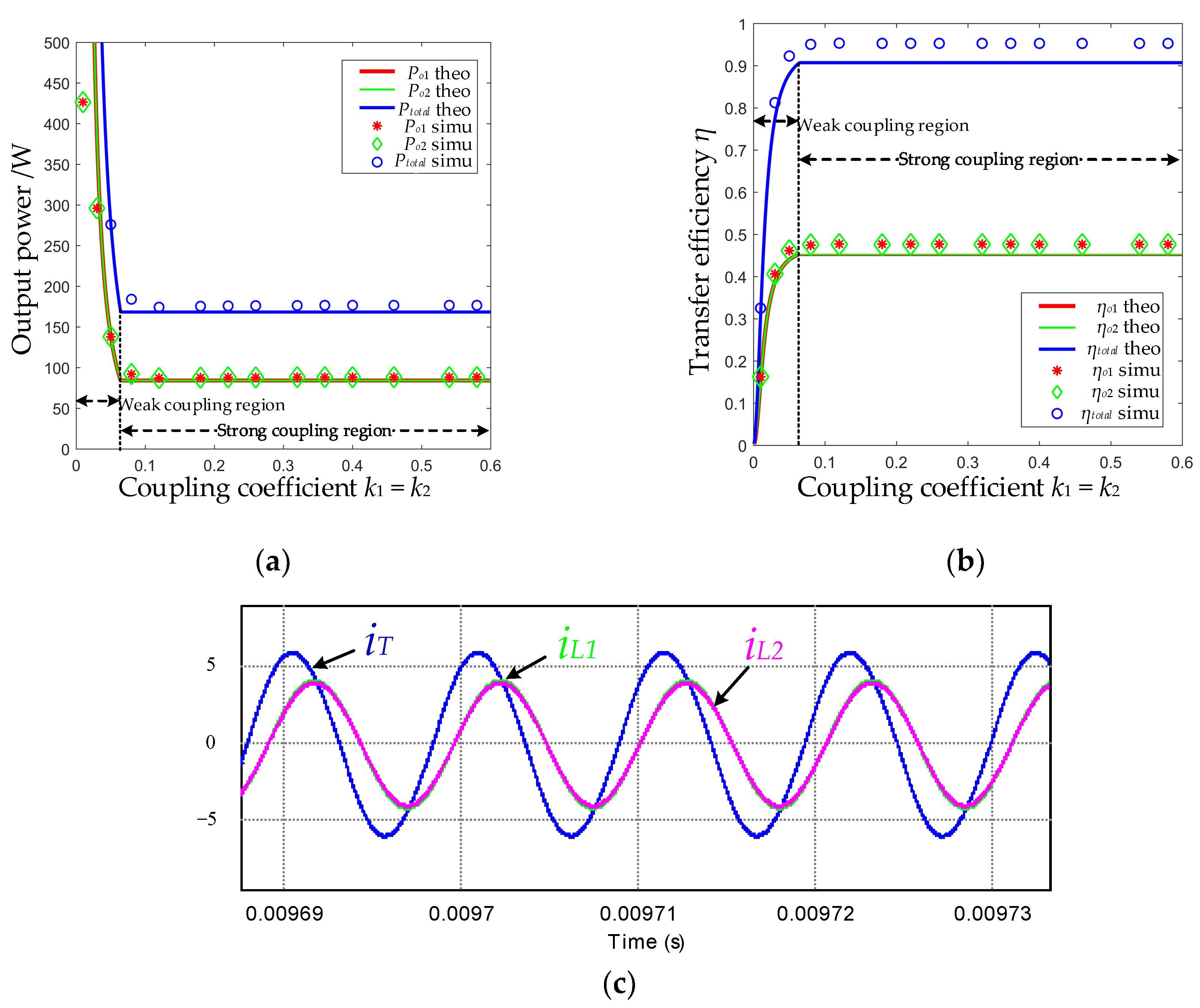
5.2. Transmission Characteristics Verificaton

Substituting the parameters of Table 2 into k c = 1 1 4 × [ 2 ( R L 1 + r L 1 ω 0 L 1 ) 2 ] 2 , the critical coupling coefficient k’c = 0.091. The simulation waveform of the output voltage vin of the full-bridge inverter and the input current iT flowing through the transmitting coil is shown in Figure 10, with a phase difference of 0°, and means generating energy. Therefore, it can be equivalent to negative resistance −RN, which is satisfied with theoretical analysis in Figure 4.
Furthermore, several different groups of k1 and k2 are randomly selected for simulation. The comparison between the simulation value and the theoretical value of the system operating angle frequency, total output power, and transfer efficiency are shown in Figure 11. Within the error range, the theoretical value is consistent with the simulation result. Figure 11a shows that the system’s operating angular frequency ω is always equal to the natural resonant angular frequency ω0 (ω0 = 2πf0 ≈ 0.628 × 10⁶ rad/s) in the weak coupling region, while in the strong coupling region, the system’s operating angular frequency is automatically adjusted as the coupling coefficients k1 and k2 change. It can be clearly seen from Figure 11b,c that the total output power of the system always remains at 175 W with constant transmission efficiency 95% when the coupling coefficients k1 and k2 change in the strong coupling region, which is not affected by the load position. However, once the system works in the weak coupling region, the total output power of the system will rise sharply, and the transfer efficiency will drop rapidly, which not only reduces the transmission performance, but also may produce a lot of heat to burn the circuit. So, in practice, it should be avoided to work in the weak coupling region.

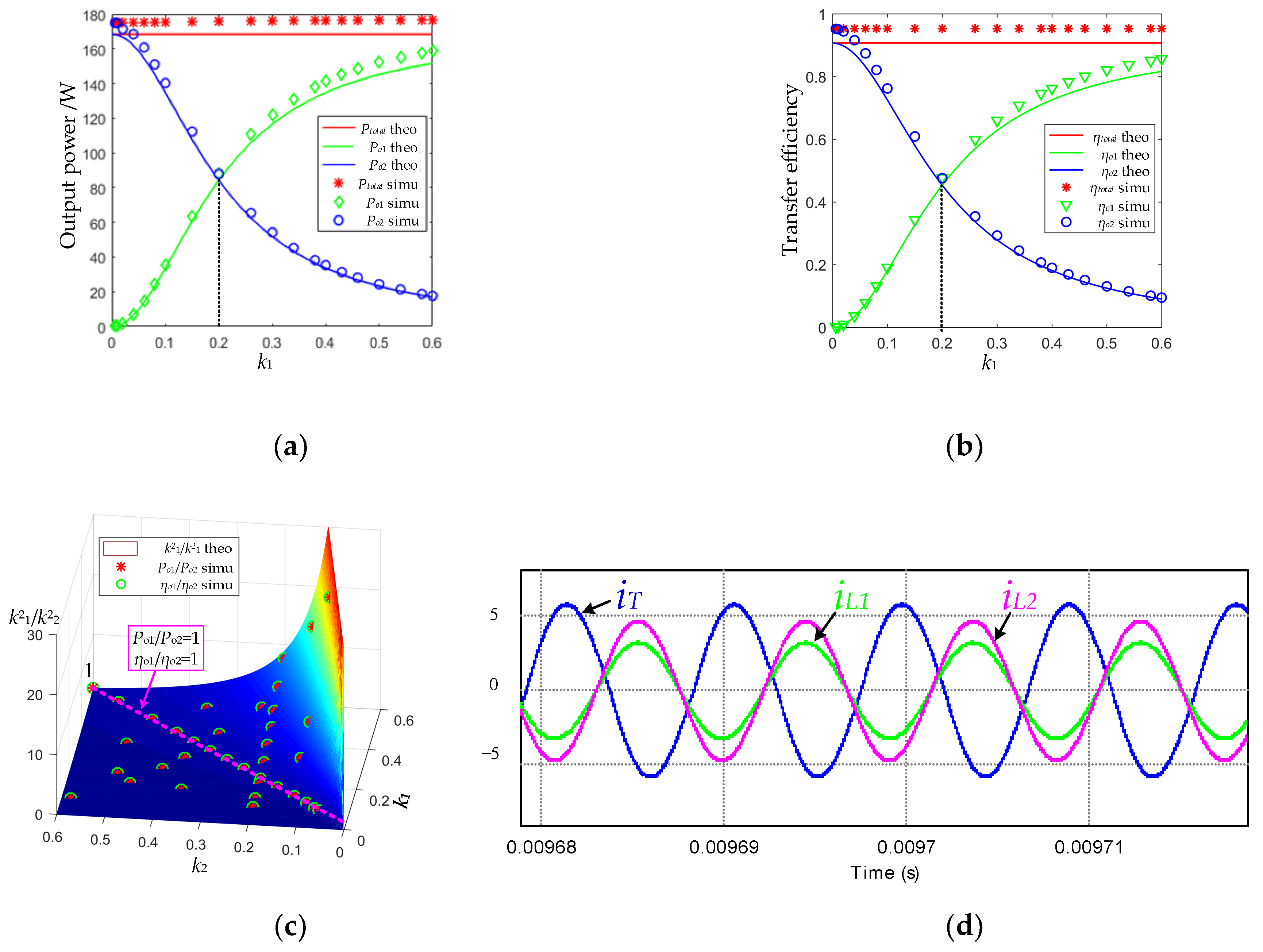
5.3. Power Distribution Verificaton

When k1 = k2, the power distribution and efficiency distribution are as shown in Figure 12a,b. The blue line and dots represent total output power and efficiency of the system, while the red and green lines and dots represent output power and efficiency of Load 1 and Load 2, respectively. As shown in Figure 12a,b, when k c 2 k 1 2 + k 2 2 < 1 , that is, strong coupling region, not only the total output power and transfer efficiency of the system remain constant, but also the output power and transfer efficiency of each load remain constant. Moreover, the output power and transfer efficiency of each load are 50% of the total output power and transfer efficiency of the system, respectively. In this case, the system and each load can achieve constant output power and constant efficiency simultaneously, which is no longer affected by the load’s position. One of the waveforms of the input current iT and the output current iL1 and iL2 is shown in Figure 12c. It can be seen that the output currents iL1 and iL2 are completely coincident, and the effective value is 4.12 A, while the effective value of the input current iT is 5.8 A. The output power Po1 = Po2 = 50% Ptotal and the efficiency ηo1 = ηo2 = 50% ηtotal of the two loads can be obtained.
When k1k2 and k c 2 k 1 2 + k 2 2 < 1 , the power distribution and efficiency distribution are as shown in Figure 13. In order to better demonstrate the power and efficiency distribution in the strong coupling region, the coupling coefficient k2 = 0.2 of Load 2 is assumed to be fixed, and the coupling coefficient k1 of Load 1 is changed from 0 to 0.6. In this case, the relationship of the output power and transfer efficiency of the two loads with the coupling coefficient k1 is shown in Figure 13a,b. It can be seen that the output power and efficiency of each load vary with the coupling coefficient and cannot be kept at a constant value, although a load position remains unchanged. Furthermore, the greater the coupling coefficient is (that is, receiver is closer to transmitter), the greater the output power and efficiency are. Further, taking any value of k1 and k2, the simulation results are as shown in Figure 13c. The ratio of output power and efficiency of each load falls on the surface of the square ratio of coupling coefficients k1 and k2. One of the waveforms of the input current iT and the output current iL1 and iL2 is shown in Figure 13d; the effective values of iT, iL1, and iL2 are 3.20 A, 4.65 A, and 5.74 A, respectively. It can be calculated that the ratio of the output power of the two loads Po1/Po2 ≈ 0.44 and the efficiency ratio ηo1/ηo2 ≈ 0.44, which is consistent with theoretical analysis.

5.4. Comparison with Existing Multi-Load WPT Systems

Table 3 compares the transfer performance of the multi-load WPT systems reported in recent years. Different from the existing multi-load WPT systems where the operating frequency is fixed and the output power and transfer efficiency are variable as loads move, the multi-load PT-WPT system proposed in this paper can automatically adjust the operating frequency according to the change of load position; at the same time, the output power and transfer efficiency of the system can be kept constant simultaneously under variable coupling coefficient.

6. Conclusions

This paper proposes a novel multi-load WPT system based on PT-symmetry, which is progress compared with the single-load PT-WPT system. Compared with the existing multi-load WPT systems, the main advantage of the proposed multi-load PT-WPT system in this paper is the ability to achieve constant output power and constant transfer efficiency of the system against variable coupling coefficients, and realize power distribution among loads simultaneously under different coupling situations. Theoretical results show that the total output power and transfer efficiency of the system can remain constant at any position in the strong coupling region. However, for a specific load, the output power and transfer efficiency will vary with the coupling coefficient. Only when all coupling coefficients are equal, that is, k1 = k2 = … = kn at any time, the system and each load achieve constant output power and constant efficiency simultaneously, and the overall output power is evenly distributed to each load. Moreover, taking a dual-load PT-WPT system as an example, the circuit simulation is carried out and the simulation results verify the theoretical analysis. There are still several challenges and open issues of the proposed multi-load PT-WPT system, such as power distribution strategy and cross-coupling effect when the load distance is relatively close. Future work will focus on the power distribution optimization when multiple portable electronic products are wirelessly charging at the same time, such as mobile phones, Bluetooth headsets, bracelets, and so on.

Author Contributions

Conceptualization, C.L. and D.Q.; Data curation, C.L.; Formal analysis, C.L.; Investigation, C.L. and M.L.; Methodology, C.L.; Project administration, D.Q.; Resources, D.Q. and B.Z.; Software, C.L.; Supervision, D.Q. and B.Z.; Validation, C.L.; Visualization, C.L.; Writing—original draft, C.L.; Writing—review & editing, D.Q. and M.L. All authors have read and agreed to the published version of the manuscript.

Funding

This research received no external funding.

Acknowledgments

This project was supported by the National Natural Science Foundation of China (Grant No. 51677074 and No. 51437005).

Conflicts of Interest

The authors declare no conflict of interest.

References

  1. Sial, A.; Singh, A.; Mahanti, A. Detecting anomalous energy consumption using contextual analysis of smart meter data. Wirel. Netw. 2019, 1–18. [Google Scholar] [CrossRef]
  2. Sial, A.; Singh, A.; Mahanti, A.; Gong, M. Heuristics-Based Detection of Abnormal Energy Consumption. Smart GIFT 2018, 21–31. [Google Scholar] [CrossRef]
  3. Li, B.; Rong, Y. Joint Transceiver Optimization for Wireless Information and Energy Transfer in Nonregenerative MIMO Relay Systems. IEEE Trans. Veh. Technol. 2018, 67, 8348–8362. [Google Scholar] [CrossRef]
  4. Chen, X.; Ng, D.W.K.; Chen, H.H. Secrecy wireless information and power transfer: Challenges and opportunities. IEEE Wirel. Commun. 2016, 23, 54–61. [Google Scholar] [CrossRef]
  5. Kim, S.; Hwang, S.; Kim, S.; Lee, B. Investigation of single-input multiple-output wireless power transfer systems based on optimization of receiver loads for maximum efficiencies. J. Electromagn. Eng. Sci. 2018, 18, 145–153. [Google Scholar] [CrossRef] [Green Version]
  6. Ahn, D.; Kim, S.M.; Kim, S.W.; Moon, J.I.; Cho, I.K. Wireless power transfer receiver with adjustable coil output voltage for multiple receivers application. IEEE Trans. Ind. Electron. 2019, 66, 4003–4012. [Google Scholar] [CrossRef]
  7. Mirbozorgi, S.A.; Bahrami, H.; Sawan, M.; Gosselin, B. A smart multicoil inductively coupled array for wireless power transmission. IEEE Trans. Ind. Electron. 2014, 61, 6061–6070. [Google Scholar] [CrossRef]
  8. Duong, Q.T.; Okada, M. Maximum efficiency formulation for multiple-input multiple-output inductive power transfer systems. IEEE Trans. Microw. Theory Tech. 2018, 66, 3463–3477. [Google Scholar] [CrossRef]
  9. Cheng, C.; Lu, F.; Zhou, Z.; Li, W.; Zhu, C.; Deng, Z.; Chen, X.; Mi, X. Load-independent wireless power transfer system for multiple loads over a long distance. IEEE Trans. Power Electron. 2019, 34, 9279–9288. [Google Scholar] [CrossRef]
  10. Lin, D.; Zhang, C.; Hui, S.Y.R. Mathematical analysis of omnidirectional wireless power transfer—part-I: Two-dimensional systems. IEEE Trans. Power Electron. 2017, 32, 625–633. [Google Scholar] [CrossRef]
  11. Lin, D.; Zhang, C.; Hui, S.Y.R. Mathematic analysis of omnidirectional wireless power transfer—part-II three-dimensional systems. IEEE Trans. Power Electron. 2017, 32, 613–624. [Google Scholar] [CrossRef]
  12. Su, M.; Liu, Z.; Zhu, Q.; Hu, A.P. Study of maximum power delivery to movable device in omnidirectional wireless power transfer system. IEEE Access 2018, 6, 76153–76164. [Google Scholar] [CrossRef]
  13. Han, H.; Mao, Z.; Zhu, Q.; Su, M.; Hu, A.P. A 3D wireless charging cylinder with stable rotating magnetic field for multi-load application. IEEE Access 2019, 7, 35981–35997. [Google Scholar] [CrossRef]
  14. Liu, G.; Zhang, B.; Xiao, W.; Qiu, D.; Chen, Y.; Guan, J. Omnidirectional wireless power transfer system based on rotary transmitting coil for household appliances. Energies 2018, 11, 878. [Google Scholar] [CrossRef] [Green Version]
  15. Zhang, W.; Zhang, T.; Guo, Q.; Shao, L.; Zhang, N.; Jin, X.; Yang, J. High-efficiency wireless power transfer system for 3D, unstationary free-positioning and multi-object charging. IET Electr. Power Appl. 2018, 12, 658–665. [Google Scholar] [CrossRef]
  16. Chabalko, M.J.; Sample, A.P. Three-dimensional charging via multimode resonant cavity enabled wireless power transfer. IEEE Trans. Power Electron. 2015, 30, 6163–6173. [Google Scholar] [CrossRef]
  17. Chabalko, M.J.; Shahmohammadi, M.; Sample, A.P. Quasistatic cavity resonance for ubiquitous wireless power transfer. PLoS ONE 2017, 12, e0169045. [Google Scholar] [CrossRef] [Green Version]
  18. Cheng, C.; Lu, F.; Zhou, Z.; Li, W.; Deng, Z.; Li, F.; Mi, C. A load-independent LCC-compensated wireless power transfer system for multiple loads with a compact coupler design. IEEE Trans. Ind. Electron. 2020, 67, 4507–4515. [Google Scholar] [CrossRef]
  19. Kim, J.; Kim, D.H.; Park, Y.J. Analysis of capacitive impedance matching networks for simultaneous wireless power transfer to multiple devices. IEEE Trans. Ind. Electron. 2015, 62, 2807–2813. [Google Scholar] [CrossRef]
  20. Fu, M.; He, Y.; Ma, C. Megahertz multiple-receiver wireless power transfer systems with power flow management and maximum efficiency point tracking. IEEE Trans. Microw. Theory Tech. 2017, 65, 4285–4293. [Google Scholar] [CrossRef]
  21. Liu, F.; Yang, Y.; Ding, Z.; Chen, X.; Kennel, R.M. A multifrequency superposition methodology to achieve high efficiency and targeted power distribution for a multi-load MCR WPT system. IEEE Trans. Power Electron. 2018, 33, 9005–9016. [Google Scholar] [CrossRef]
  22. Zhang, Z.; Pang, H.; Wang, J. Multiple objective-based optimal energy distribution for wireless power transfer. IEEE Trans. Magn. 2018, 54, 8600205. [Google Scholar] [CrossRef]
  23. Fu, M.; Yin, H.; Liu, M.; Wang, Y.; Ma, C. A 6.78 MHz multiple-receiver wireless power transfer system with constant output voltage and optimum efficiency. IEEE Trans. Power Electron. 2018, 33, 5330–5340. [Google Scholar] [CrossRef]
  24. Walasik, W.; Ma, C.; Litchinitser, N.M. Nonlinear parity-time-symmetric transition in finite-size optical couplers. Opt. Lett. 2015, 40, 5327–5330. [Google Scholar] [CrossRef]
  25. Elganainy, R.; Makris, K.G.; Khajavikhan, M.; Musslimani, Z.H.; Rotter, S.; Christodoulides, D.N. Non-Hermitian physics and PT symmetry. Nat. Phys. 2018, 14, 11–19. [Google Scholar] [CrossRef]
  26. Schindler, J.; Li, A.; Zheng, M.C.; Ellis, F.M.; Kottos, T. Experimental study of active LRC circuits with PT-symmetries. Phys. Rev. A 2011, 84, 040101. [Google Scholar] [CrossRef] [Green Version]
  27. Lin, Z.; Schindler, J.; Ellis, F.M.; Kottos, T. Experimental observation of the dual behavior of PT-symmetric scattering. Phys. Rev. A 2012, 85, 50101. [Google Scholar] [CrossRef] [Green Version]
  28. Assawaworrarit, S.; Yu, X.; Fan, S. Robust wireless power transfer using a nonlinear parity–time-symmetric circuit. Nature 2017, 546, 387–390. [Google Scholar] [CrossRef]
  29. Zhou, J.; Zhang, B.; Xiao, W.; Qiu, D.; Chen, Y. Nonlinear parity-time-symmetric model for constant efficiency wireless power transfer: Application to a drone-in-flight wireless charging platform. IEEE Trans. Ind. Electron. 2019, 66, 4097–4107. [Google Scholar] [CrossRef]
  30. Hou, Y.; Lin, M.; Chen, W.; Yang, X. Parity-time-symmetric wireless power transfer system using switch-mode nonlinear gain element. In Proceedings of the 2018 IEEE International Power Electronics and Application Conference and Exposition (PEAC), Shenzhen, China, 4–7 November 2018. [Google Scholar] [CrossRef]
  31. Liu, F.; Yang, Y.; Jiang, D.; Ruan, X.; Chen, X. Modeling and optimization of magnetically coupled resonant wireless power transfer system with varying spatial scales. IEEE Trans. Power Electron. 2016, 32, 3240–3250. [Google Scholar] [CrossRef]
  32. Shu, X.; Zhang, B. Single-wire electric-field coupling power transmission using nonlinear parity-time-symmetric model with coupled-mode theory. Energies 2018, 11, 532. [Google Scholar] [CrossRef] [Green Version]
Figure 1. Schematic of single-load PT-WPT system using series-series topology with nonlinear negative resistance represented in operational amplifier form: (a) the circuit topology; (b) the equivalent circuit diagram.
Energies 13 03260 g001
Figure 2. Curve of the relationship between system transmission characteristics and coupling coefficient k: (a) operating angular frequency ω; (b) output power and transfer efficiency. (The system parameters are: the effective value of input voltage Vin = 50 V, the natural resonance frequency f0 = 100 kHz, the internal resistance rT = rR = 0.5 Ω, and the load resistance RL = 10 Ω).
Energies 13 03260 g002
Figure 3. Schematic of multi-load PT-WPT system using series-series topology with self-oscillating full-bridge inverter: (a) system structure with n loads; (b) equivalent circuit of the dual-load PT-WPT system.
Energies 13 03260 g003
Figure 4. The voltage and current of the nonlinear negative resistance.
Energies 13 03260 g004
Figure 5. Theoretical values of the operating angular frequency ω.
Energies 13 03260 g005
Figure 6. Coupling coefficient between two coils at different positions: (a) any position of the two planar coils; (b) curve of coupling coefficient, offset angle, and axial distance.
Energies 13 03260 g006
Figure 7. Schematic diagram of power distribution when k1 = k2: (a) loads position; (b) output power and transfer efficiency of system and each load. (In the figure, “theo” is the abbreviation of “theory”, which represents the theoretical value, the same below.)
Energies 13 03260 g007
Figure 8. Schematic diagram of power distribution when k1k2: (a) Loads position; (b) power distribution when k1 changes and k2 = 0.1 is fixed.
Energies 13 03260 g008
Figure 9. Simulation circuit of PT-WPT system with two loads.
Energies 13 03260 g009
Figure 10. Voltage and current simulation waveform of full-bridge inverter.
Energies 13 03260 g010
Figure 11. Transmission characteristics of double-load PT-WPT system: (a) operating angular frequency ω; (b) total output power Ptotal; (c) total transfer efficiency ηtotal.
Energies 13 03260 g011
Figure 12. Power distribution and efficiency distribution when k1 = k2: (a) power distribution; (b) efficiency distribution; (c) waveform of input and output current when k1 = k2 = 0.15. (In the figure, “simu” is the abbreviation of “simulation”, which represents the simulation results, the same below.)
Energies 13 03260 g012
Figure 13. Power distribution and efficiency distribution when k1k2: (a) power distribution; (b) efficiency distribution; (c) waveform of input and (d) output current when k1k2, and k1 = 0.1, k2 = 0.2.
Energies 13 03260 g013
Table 1. Comprehensive comparison of single-load PT-WPT and dual-load PT-WPT system (working in the strong coupling region and i = 1, 2).
ItemsSingle-Load PT-WPTDual-Load PT-WPT
PT symmetry conditions { ω T = ω R = ω 0 R N + r T L T = R L + r R L R { ω T = ω 1 = ω 2 = ω 0 R L 1 L 1 = R L 2 L 2 R N + r T L T = R L 1 + r L 1 L 1 = R L 2 + r L 2 L 2
Coupling coefficient condition 1 1 4 × [ 2 ( R L + r R ω 0 L R ) 2 ] 2 k 2 1 1 1 4 × [ 2 ( R L 1 + r L 1 ω 0 L 1 ) 2 ] 2 k 1 2 + k 2 2 1
Total output power R L V i n 2 L T ( R L + r R ) 2 L R + 2 ( R L + r R ) r T + L R L T r T 2 R L 1 V i n 2 L T ( R L 1 + r L 1 ) 2 L 1 + 2 ( R L 1 + r L 1 ) r T + L 1 L T r T 2
Total transfer efficiency R L L T r T L R + L T ( R L + r R ) R L 1 L T r T L 1 + L T ( R L 1 + r L 1 )
ith load output power- R L i V i n 2 k i 2 / ( k 1 2 + k 2 2 ) L T ( R L i + r L i ) 2 L i + 2 ( R L i + r L i ) r T + L i L T r T 2
ith load efficiency- k i 2 k 1 2 + k 2 2 R L i L T r T L i + L T ( R L i + r L i )
Table 2. Parameters of the dual-load PT-WPT system.
ParametersValuesParametersValuesParametersValues
VDC/V50L1/μH183.5L2/μH195.6
LT/μH181.7C1/nF13.8C2/nF12.95
CT/nF13.94RL110RL210.66
rT0.53rL10.5rL20.52
Table 3. Comparison of multi-load WPT systems.
ReferenceOperating FrequencyTransmitting Coil StructureCoil SizeOperating ConditionOutput Power and Efficiency
[9]200 kHzRepeater coils16 × 16 cmFixed loadUnstable
[13]20 kHzTwo orthogonal square coils30 × 30 cmMovable loadUnstable
[14]1 MHzRotating circular coilr = 32 cmFixed loadUnstable
[15]50 kHzHelmholtz coils20 × 20 × 14 cmMovable loadUnstable
[17]1.32 MHzMetallic chamber4.9 × 4.9 × 2.3 mMovable loadUnstable
This workAdjust around 100 kHzSingle plane coilr = 26 cmMovable loadConstant

