Abstract
Previous studies have shown that different parameters such as reservoir conditions (e.g., pressure, temperature, and brine chemistry) and wellbore hydraulics influence the scaling tendency of minerals on the surfaces of completion tools in conventional resources. Although different studies have investigated the suitable conditions for the precipitation of scaling minerals, there is still a lack of understanding about the composition of the scaling materials deposited on the surfaces of completion tools in thermal wells. In this study, we presented a laboratory workflow combined with a predictive toolbox to evaluate the scaling tendency of minerals for different downhole conditions in thermal wells. First, the scaling indexes (SIs) of minerals are calculated for five water samples produced from thermal wells located in the Athabasca and Cold Lake areas in Canada using the Pitzer theory. Then, different characterization methods, including scanning electron microscopy (SEM) with energy dispersive X-ray spectrometry (EDS), inductively coupled plasma mass spectrometry (ICP-MS) and colorimetric and dry combustion analyses, have been applied to characterize the mineral composition of scale deposits collected from the surfaces of the completion tools. The results of the SI calculations showed that the scaling tendency of calcite/aragonite and Fe-based corrosion products is positive, suggesting that these minerals can likely deposit on the surfaces of completion tools. The characterization results confirmed the results of the Scaling Index calculations. The SEM/EDS and ICP-MS characterizations showed that carbonates, Mg-based silicates and Fe-based corrosion products are the main scaling components. The results of dry combustion analysis showed that the concentration of organic matter in the scale deposits is not negligible. The workflow presented in this study provides valuable insight to the industry to evaluate the possibility of scaling issues under different downhole conditions.
1. Introduction
Steam-assisted gravity drainage (SAGD) wells are a critical part of the energy supply chain in Canada. The oil production rate from these thermal wells is generally lower than that from conventional wells. The oil flow rate in these wells is affected by scale formation and plugging material precipitation. These materials create a barrier for the oil flow, leading to a reduction in the oil flow rate.
The main reason for downhole solid precipitation is the disturbance of the thermodynamic equilibrium that exists between underground fluids and their surroundings, which occurs due to drilling and production operations. These deposits may have an organic nature, when they are generally called “wax” or “asphaltenes” [1,2,3], or may have an inorganic nature, when they are called “scale” [4,5]. The thickness of the developed scale in thermal wells is variable, depending on the pressure, temperature and water chemistry of the well; however, in general, the thickness may range from 0.7 cm to more than 3 cm, leading to a 10–45% fluid restriction [6]. Furthermore, the type of the scales used in the petroleum industry varies considerably. Habibi et al. (2020) [7] categorized the mineral composition of scale deposits removed from completion tools. They showed that the inorganic scale deposits are mainly silicates, carbonates and corrosion products. The iron-based scales are reported to be a result of the corrosion in the tubulars. The location of scale deposition may be anywhere inside the formation—e.g., around the wellbore, in the production string or inside perforations—which may lead to a considerable decline of production [8]. In addition to the loss of production, as displayed in Figure 1a, subsequent scale removal or the application of scale inhibitors may cost up to USD 1.4 billion annually [9]. As depicted in Figure 1b, of the major production loss factors in the North Sea region, scale contributes to 28%, and a similar trend is expected for mature fields around the world [8].
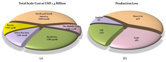
Figure 1.
(a) World-wide cost of scale treatment and (b) production loss due to different processes in the North Sea (modified after [8]).
Cleaning methods are essential for increasing or maintaining production rates and lowering the damage to the downhole equipment. They are generally divided into two main groups: chemical and mechanical. The chemical methods of scale removal depend on the solubility of scale deposits in acids, water or other chemicals. For example, calcite, sulfide, oxide, dolomite and hydroxide scales are sensitive to pH, meaning that acids (usually HCl) can dissolve these components. On the other hand, sulfates (calcium sulfate, barium sulfate, strontium sulfate, or barium strontium sulfate), phosphates and ferricyanide are insensitive to pH, meaning that other chemicals—e.g., chelating agents—can dissolve these components [10]. Moreover, iron-based scale deposits are the corrosion products of metallic surfaces due to the presence of dissolved oxygen, hydrogen sulfide [11] and dissolved CO, all of which are acid-soluble. Using chemical methods for cleaning the thermal wells may be challenging; for instance, acids can corrode the chrome surfaces of downhole equipment even at temperatures higher than 360 K.
The mechanical methods include a wide range of techniques, such as re-perforating, reaming, sonic methods and scrapers. A major challenge in mechanical scale removal in SAGD wells is that the scale deposits not only form inside tubulars but also develop inside the sand control devices’ openings and plug them. The scale formed inside production pipes could be removed by typical mechanical methods; however, to remove scales inside slots, other advanced and special techniques, such as electro-hydraulic stimulation tools which generate strong shockwaves, can be employed [7]. If none of the cleaning procedures prove to be effective in conventional wells, several techniques can be employed. These include (i) side tracking (deviation of the well), (ii) deepening of the well, (iii) installing an orifice at the wellhead (to provide higher pressure in the well and reduce scale formation), (iv) increasing production casing diameter and (v) spreading the scale formation zone into places where cleaning is possible (e.g., from inside the reservoir to inside the tubing). Finding the best method for cleaning the plugged thermal wells is not straightforward as different parameters affect the scaling behavior of minerals. To select a proper remedial technique for cleaning the plugged wells, it is necessary to (i) improve our understanding of how reservoir conditions (temperature, pressure and water chemistry) affect the precipitation process and (ii) more precisely measure the mineral composition of the plugging materials.
In this study, we presented a laboratory workflow for the characterization of the mineralogy of scale deposits combined with a predictive toolbox for estimating the scaling tendency of minerals for different produced water samples. First, the predictive toolbox was used for water samples collected from five thermal wells located in the Athabasca and Cold Lake areas (with a typical reservoir pressure of 800 kPa, an initial reservoir temperature of 8 °C, an operating temperature ranging from 90–180 °C, an oil API gravity ranging from 8.05–10.71, an oil viscosity at 24 °C ranging from 65–323 Pa.s and an average oil saturation of 0.75). To predict the scaling tendency of the minerals dissolved in water solution, we used the PHREEQC 3, (U.S. Geological Survey, Denver, CO, USA) software package. This package is free of charge and widely used as software in the field of geo-chemistry. More details about this software are presented elsewhere [12]. Second, to implement the laboratory workflow, we analyzed five solid scale samples collected from thermal wells. These materials were attached to the surfaces of the completion tools. Finally, we compared the characterization and prediction results.
2. Pitzer Theory
The Pitzer theory, as a thermodynamic model, has been used by different geo-chemical software to model the scaling tendency of minerals present in an aqueous solution [13,14,15,16,17,18]. This model uses virial coefficients depending on pressure, temperature and ionic strength. Therefore, it can predict the thermodynamic properties of minerals for a wide range of temperatures, pressures and ionic strengths of a solution [19,20,21]. The saturation ratio (SR) is a thermodynamic parameter used to predict the scaling tendency of minerals dissolved in the aqueous phase (Equation (1)) [8]. The SR for each mineral is defined as the ion activity product divided by its thermodynamic solubility product (Equations (2) and (3)). This ratio reflects the composition of a product in a real state to that in a saturation state.
where and are cationic and anionic species in the aqueous phase, respectively; n, and are stoichiometric coefficients; and are the activity of cationic and anionic species, respectively; , , and are the solubility products (depending on the temperature and pressure), the molality of the cation and the molality of the anion, respectively; and and are the activity coefficients of the cation and anion, respectively, which are calculated based on the excess Gibbs free energy. Details about calculating the activity coefficient of ions are presented elsewhere [22].
An important limitation of the Pitzer theory is the lack of available virial coefficients at high pressures and temperatures. Therefore, the prediction of minerals solubility under these conditions may lead to inaccuracies. Several studies have investigated the mineral solubility for specific systems to measure the virial coefficients used in the Pitzer theory [16,23,24,25]. For example, Shi et al. (2012) [26] showed that predicting the barite solubility without considering the pressure dependency of the virial coefficients resulted in a barite solubility 27% less than the measured value at 110.3 MPa and 200 °C in 6 m NaCl solutions. Therefore, more experimental data at high pressures and temperatures are needed to extend the applicable range of the Pitzer theory.
The SI of a mineral is the logarithm of the SR Equation (4). There are three different scenarios for an aqueous system with dissolved minerals, as shown in Equation (5). The precipitation of a mineral can occur when a solution is supersaturated with that mineral; otherwise, the mineral stays soluble in the aqueous phase.
Calculating the SI for minerals dissolved in reservoir brine (high electrolyte solution) can provide useful information to better understand the possibility of mineral precipitation under reservoir conditions. In this study, we calculated the SI for minerals dissolved in different water samples in a wide range of temperatures (288–498 K).
3. Materials
Five solid scale samples were collected from different completion tools used in thermal wells. These tools were plugged during oil production due to the deposition of these minerals. Hydrofluoric acid and nitric acid were used to dissolve scales for ICP-MS analysis. Atropine was used as an external standard in the dry combustion tests. To perform each step of characterization, samples were prepared with a specific procedure, as presented in the methodology section.
4. Methodology
A laboratory protocol was implemented to characterize the mineral composition of the scale deposits. Figure 2 shows a flowchart of the characterization methods used to evaluate the mineralogy of these samples collected from the completion tools in thermal wells. This protocol is composed of four different steps: (I) SEM/EDS analysis to visualize and evaluate the elemental spectrum of the scale deposits, (II) ICP-MS analysis to quantify metallic components, (III) colorimetric analysis to quantify the sulfate and chloride components and (IV) dry-combustion analysis to quantify the organic and inorganic carbon contents of these samples.
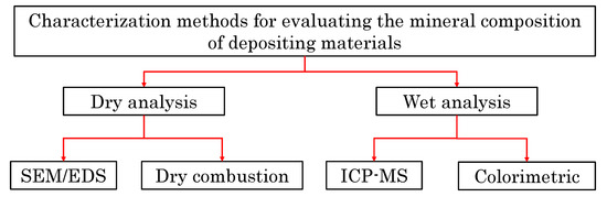
Figure 2.
Characterization methods used to evaluate the mineral composition of materials deposited on the surfaces of the completion tools.
4.1. SEM/EDS Analysis
SEM/EDS analysis was used to visualize the scale sample and evaluate its elemental structure. Samples collected from the completion tools were dried and crushed using a pestle and mortar to prepare the powder required for the analysis. A Zeiss Sigma Field Emission Scanning Electron Microscope (FESEM-300 VP) was used to visualize the scale samples. The microscope was equipped with a Bruker EDS beam to evaluate the elemental analysis of the samples.
4.2. ICP-MS Analysis
A Perkin Elmer’s Elan 6000 ICP-MS was used to quantify the metallic components of the samples. To perform the ICP-MS analysis, a series of preparation steps was performed as follows.
- The solid sample was crushed using a pestle and mortar to prepare powder.
- To prepare the liquid solution, 0.2 g of the powder was mixed with 8 mL hydrofluoric acid and 2 mL nitric acid in a container.
- The mixture was placed on a hotplate at 130 °C until it became completely dry.
- Five milliliters of hydrochloric acid and 5 mL nitric acid were added to the container. The mixture was heated at 130 °C until it became dry again.
- Ten milliliters of nitric acid (8N) was added to the container, and the mixture was heated at 130 °C for several hours. Acid washing and drying steps with different portions of hydrofluoric and nitric acids were performed to ensure that the scale deposits were completely dissolved in acids.
- To prepare a diluted sample, the mixture and deionized water were mixed in a 15 mL tube.
- One milliliter of the diluted sample was mixed with 0.1 mL nitric acid, 0.1 mL internal standards (In, Bi, and Sc), and 8.8 mL deionized water. These standards were added to ensure that the instrument accurately measured the ions concentration. The final solution was shaken thoroughly to prepare a uniform sample for the ICP-MS analysis.
4.3. Colorimetric Analysis
To evaluate the concentration of sulfate (SO) and chloride (Cl) species, a Thermo Gallery Plus Beermaster Autoanalyzer was used. This characterization method is based on color reactions. First, the solid powder (the preparation steps for the powder was the same as previous analyses) was mixed with deionized water at a 1:5 weight ratio. Since the amount of available solid sample was limited, the ratio of 1:5 was selected; however, a weight ratio of 1:2 is recommended if there is sufficient solid sample available. Second, the mixture was shaken for 30 min, centrifuged at 6000 rpm and filtered using a syringe with a 0.45 m pore size. Third, the sample and reagents (depending on the characterization method for each component) were injected into the reaction cuvettes. Colored complexes were generated after chemical reactions. The intensity of the color change in the mixture depended on the concentration of solutes (Beer–Lambert law) [27,28]. Fourth, this intensity was measured by light absorbance at a specific wavelength (430 nm for SO and 510 nm for Cl). The ferrithiocyante method (US Environmental Protection Agency (EPA) Method 325.2) [29] and barium chloride turbidimetric method (EPA Method 375.4) [30] were used as references for the characterization of Cl and SO, respectively. Due to the limited available amount of solid samples, we could not use this instrument to quantify the concentration of HCO and CO. To distinguish the inorganic and organic carbon contents of the solid samples, dry combustion analysis was performed.
4.4. Dry Combustion Analysis
To evaluate the total carbon (TC) and total organic carbon (TOC) contents in the solid samples, a Thermo FLASH 2000 Organic Elemental analyzer was used. The flash combustion method is the basis of this instrument. The complete combustion of the sample was achieved by placing the sample into a combustion tube. Several combustion reactions occurred in the tube at high temperatures (1800–2000 °C); as a result, the TC content was converted to CO. Then, the CO gas was separated in a chromatographic column followed by quantitative detection by a thermal conductivity detector. More details about the operational procedure of this instrument are presented elsewhere [31,32]. Atropine was used as an external standard. The TC content of the atropine (with 70.56 wt% TC) was measured and compared with its reported TC value.
To quantify the TOC contents, several steps were performed. First, the weight of the solid sample was measured in an open cell, followed by mixing with 50 L hydrochloric acid. Then, the mixture was dried at 40 °C overnight. The difference between TC and TOC is the total inorganic carbon (TIC) content. This parameter represents bicarbonate and carbonate together.
5. Results and Discussions
This section presents the prediction and characterization results. The SIs of minerals for the five water samples produced from the thermal wells and characterization results for five solid samples are presented.
5.1. SI Prediction
To calculate the SIs of minerals in an aqueous phase, the water chemistry analysis of the water sample was required. Table 1 lists the chemical analysis of the produced water samples from five thermal wells in the Athabasca and Cold Lake areas.

Table 1.
Water chemistry analysis of the produced water from five thermal wells located in the Athabasca and Cold Lake areas. Values are in ppm.
Figure 3 shows the SI versus temperature for the water samples listed in Table 1. Since the constituents of water samples for wells A and B are the same, the scaling minerals are similar for these water samples. The main difference between these water samples is the concentration of species. The concentration of all species in sample A is higher than that of water sample B, except for iron (Fe). First, the main scaling minerals for samples A and B are iron-based components; these include hematite (FeO), goethite (FeOOH) and iron (III) hydroxide (Fe(OH)). The corrosion of the completion tools can result in the formation of iron-based products in the water solution. One source for corroding iron is the dissolved oxygen in the process of formation or injected water and very hot gases [8]. However, the steam used in the SAGD process is deaerated. Therefore, it provides a limited amount of oxygen for the corrosion of metal surfaces. Another source for corroding iron in SAGD operations is acid gases (CO and HS). These gases are the product of a chemical reaction between the steam condensate and sulfur, nitrogen and oxygen components present in the bitumen when it is heated up to 180 °C [33]. Table 2 lists the available data in the literature about the volume of produced CO and HS per m of bitumen in the Athabasca and Cold Lake areas [34]. The dissolution of acid gases in water under downhole conditions can result in the corrosion of metal surfaces. It should be also noted that the pH values listed in Table 1 are the results of the water analysis performed at the surface conditions. Acidic water (low pH values) at elevated temperatures and pressures is expected as the dissolution of acid gases in water under downhole conditions is higher than that under surface conditions [35]. Second, barite (BaSO) can also precipitate when T < 330 K. Third, SI values for calcite and aragonite increase when increasing the temperature. Calcite (hexagonal) and aragonite (orthorhombic) are two carbonate polymorphs [36]. The maximum SI values for calcite and aragonite are 1.4 and 1.46 at 498 K, respectively.
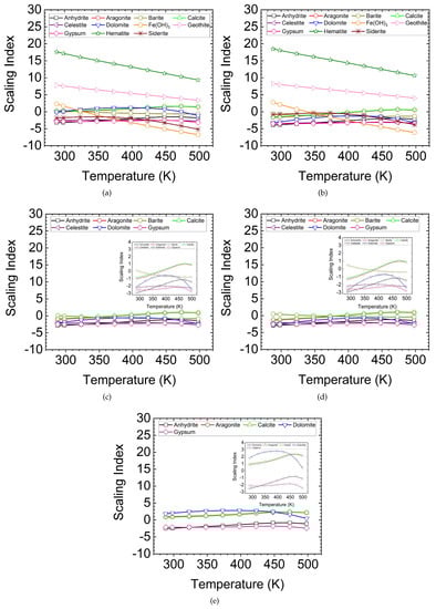
Figure 3.
Scaling Index versus temperature for (a) well A, (b) well B, (c) well C, (d) well D and (e) well E. The main scaling minerals for samples A and B are FeO, FeOOH and Fe(OH). Samples C and D are Fe-free samples. For these samples, CaCO can precipitate. CaMg(CO) can precipitate from sample E when T < 398 K.
Table 2.
Average volume of CO and HS produced per m of bitumen at 240 °C. These data were extracted from core analysis [34].
Water samples C and D are iron-free samples. SI values for calcite and aragonite are positive, suggesting the formation of carbonate scale. Moreover, the SI for barite in sample D is positive when T < 330 K. This indicates that barite is soluble in water at T > 330 K.
The water sample E has the highest Mg and Ca concentrations among all water samples, implying the formation of dolomite in the temperature range of 288–498 K, as shown by the positive SI in this range (Figure 3e). The SI of dolomite for well E follows a nonlinear trend, increasing with the increasing temperature up to 398 K. The maximum SI is 2.79 at T = 398 K; then, it decreases with a further increase in temperature. This result shows the possibility of dolomite precipitation at 398 K. Although no data are reported in the literature about dolomite precipitation at the laboratory-scale, it can precipitate over a long period of time at the field scale [15].
5.2. Characterization of Scale Deposits
In this section, the characterization results of the scale samples deposited on the surfaces of the completion tools are presented. These characterization analyses include SEM/EDS, ICP-MS, colorimetric and dry combustion analyses.
5.2.1. SEM/EDS Analysis
Figure 4 shows the SEM image and EDS spectrum for different regions of the first scale sample. Each region has a specific spectrum composed of different peaks. This variation shows the mineral heterogeneity of the scale samples. This observation is in agreement with previous studies that showed the mineral heterogeneity of depositing minerals [7,37]. In this sample, there are four regions with different components: (1) organic matter, (2) iron sulfide, (3) Mg-based silicates and (4) calcite/aragonite.
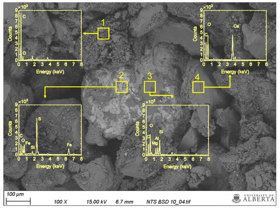
Figure 4.
The EDS spectrum for four different regions in the first scale sample. Region 1 has a strong carbon peak with a very small oxygen peak. This indicates the presence of organic matter in the scale. Region 2 has strong sulfur and iron peaks, suggesting the presence of iron sulfide in this region. Region 3 has aluminum, magnesium and silicon peaks, suggesting the presence of Mg-based silicate scales. Region 4 has calcium, oxygen and carbon peaks, indicating the main components of calcite/aragonite minerals.
Figure 5 shows the SEM image and EDS spectrum of the second scale sample. Two different regions are highlighted with yellow squares. Region 1 is rich in iron and oxygen, which suggests the presence of corrosion products (hematite, goethite and iron (III) hydroxide) in this region. Silicon, aluminum and oxygen peaks are strong in region 2, which implies the presence of silicate minerals. The visualization results of SEM/EDS analysis are in agreement with the scaling tendency results calculated based on the chemical analysis of the water samples produced from thermal wells and the Pitzer theory. Calcite/aragonite, iron-based products and silicates are the main scaling minerals, as indicated by the positive SI values.
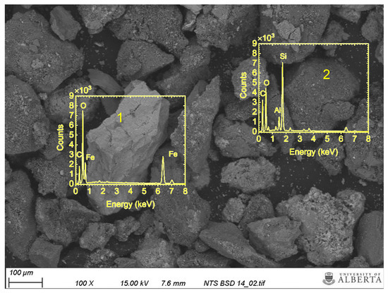
Figure 5.
The EDS spectrum for two regions in the second scale sample. Region 1 has iron and oxygen peaks. This suggests the presence of iron oxide. Region 2 has aluminum, magnesium, and silicon peaks, suggesting the presence of silicate scales.
5.2.2. ICP-MS Analysis
Table 3 lists the concentration of metallic ions present in the five solid samples collected from the completion tools in the thermal wells. There is a significant difference between the ion concentrations in the produced water samples and scale deposits. This can be explained by the precipitation of minerals on the surfaces of the completion tools under downhole conditions during the production period and the reduction of ion concentration in the produced water.
Table 3.
The concentration of metallic ions extracted from solid scale samples by ICP-MS analysis.
The most abundant element is Ca, with a concentration in the range of 189,722–231,151 ppm. This high Ca concentration indicates the presence of Ca-based components in the scale deposits. These components could be calcite and aragonite. The second element is Fe, and its concentration changes from 14,487 to 89,447 ppm. It is unlikely that the source of this amount of iron is the reservoir brine because the iron concentration in the reservoir brine is typically less than 0.1 ppm. The main source of iron (Fe(OH), FeOOH, FeO) is the corrosion of the metallic surfaces of the tubular. Another possibility could be the detachment of rock fragments such as siderite (FeCO) from the rock surface and their accumulation on the scale deposits. Therefore, several types of iron-based components can deposit on the surfaces of the completion tools, resulting in the plugging of the open-to-flow areas and a subsequent reduction in the oil production rate.
The third element is Mg, with a concentration in the range of 5119–7763 ppm. The presence of Mg shows the precipitation of Mg-based minerals, such as dolomite (as shown in Figure 3e), and Mg-based silicate deposits (as shown in region 3 in Figure 4). The fourth abundant element is Sr. The presence of 2428–2781 ppm of Sr is sufficient for the formation of celestite (SrSO) scale during the oil production. The remaining elements—i.e., Ti, Cr, Mn, Ni and Cu—are the components of completion tool materials which corroded during the oil production.
5.2.3. Colorimetric Analysis
Table 4 lists the concentration of sulfate and chloride species present in the scale deposits. The significant difference between the ICP-MS and colorimetric results may be related to the quantification methodology used for these minerals. The Cl concentration is in the range of 1.44–6.63 ppm. This concentration is much smaller than the concentration of metallic ions listed in Table 3. This indicates that it is improbable to observe the deposition of halite (NaCl). This component is highly soluble in water. The Na concentration reported by ICP-MS analysis is in the range of 917–2534 ppm. If all the Cl is consumed to produce halite scale, less than 0.5% of Na is used. Therefore, the rest of the Na could be a component of phyllosilicate minerals (clays). Next, the sulfate concentration changes from 3.75 to 16.69 ppm. The higher sulfate concentration compared with chloride suggests that the precipitation of sulfate-based minerals is greater than for chloride. Considering the metallic ion concentration obtained from ICP-MS analysis (Table 3), the sulfate-based minerals could be BaSO, CaSO, and CaSO·2HO. The next step is to evaluate carbon-based minerals by performing dry combustion analysis.
Table 4.
Concentrations of sulfate (SO4−2) and chloride (Cl−1) extracted from five solid samples using the colorimetric method.
5.2.4. Dry Combustion Analysis
Table 5 lists the TC, TOC and TIC contents evaluated for five scale deposits using the dry combustion method. TIC is the difference between TC and TOC. Since a limited amount of the scale deposits was available for the analysis, we could not perform the extraction analysis to separate carbonate (CO) from bicarbonate (HCO). First, the TC concentration for atropine (external reference standard) is 70.54 wt%. This value is very close to the known value (70.56 wt% for TC). Next, the TOC content is in the range of 9.15–11.5 (w/w)%. The oil API for thermal wells is low, meaning that heavy oil is produced from these wells. The source of organic carbon could be the heavy components of the produced oil or bitumen, such as asphaltenes, and resins precipitated on the surfaces of the tubular during the oil production. The results of the saturates, aromatics, resins and asphaltenes (SARA) analysis for the Athabasca and Cold Lake bitumens are reported in the literature [38,39]. The concentration of asphaltenes and resins for the Athabasca and Cold Lake bitumens are 43.03 and 40.06 wt%, respectively [38]. Region 1, highlighted in Figure 4, shows the existence of organic matter in the scale deposits. Mixing the organic matter with inorganic scales results in formation of more complex deposits in terms of physicochemical properties compared to pure inorganic scale deposits. Moreover, the concentration of TIC changes from 5.31 to 6.08 (w/w)%. This shows that up to 6.08 wt% of scale deposits could be carbonate and bicarbonate-based components. These components could be aragonite, calcite, magnetite and siderite based on the concentration of metallic ions presented in Table 3.
Table 5.
Total carbon (TC), total organic carbon (TOC) and total inorganic carbon (TIC) contents evaluated by dry combustion analysis.
6. Conclusions
In this study, we presented a series of characterization methods (SEM/EDS, ICP-MS, colorimetric and dry combustion analyses) to evaluate the mineral composition of five scale samples deposited on the surfaces of completion tools in thermal wells. We also calculated the scaling tendency of minerals in five water samples produced from the thermal wells in the Athabasca and Cold Lake areas. A summary of the main conclusions is provided below:
- The results of the scaling index prediction for minerals showed that Fe-based corrosion products and calcite/aragonite could be the main depositing materials.
- The SEM/EDS analysis visualized the heterogeneity of the scale deposits. The main components were organic matter, Fe-based corrosion products, Mg-based silicates and calcite/aragonite. The ICP-MS analysis agrees with the SEM/EDS visualization results.
- The results of the dry combustion analysis demonstrated the presence of organic matter in the scale deposits. The concentration of organic matter was not negligible; therefore, it is expected that the mixing of the organic matter and inorganic minerals leads to more complex structures of these deposits compared to pure inorganic deposits.
Author Contributions
Conceptualization, A.H., M.S. and C.E.F.; methodology, A.H., M.S. and H.Z.; software, A.H.; validation, M.R., C.E.F. and M.M.; formal analysis, A.H.; investigation, A.H., M.R. and V.F.; data curation, A.H. and M.M.; writing–original draft preparation, A.H. and M.R.; writing–review and editing, A.H., M.R., M.S., V.F. and H.Z.; visualization, A.H. and M.R.; supervision, C.E.F., M.M., V.F., M.S. and H.Z.; funding acquisition, C.E.F. and V.F. All authors have read and agreed to the published version of the manuscript.
Funding
This research was funded by Blue Spark Energy, RGL Reservoir Management Inc., and the Mitacs Postdoctoral Award.
Acknowledgments
The authors thank Blue Spark Energy and RGL Reservoir Management Inc. for their permission to publish this paper. The financial support provided by Mitacs through the Accelerate program is also acknowledged.
Conflicts of Interest
The authors declare no conflict of interest.
References
- Al-Qasim, A.; Alsubhi, M.; Al-Anazi, A. Heavy Organic Deposit Formation Damage Control, Analysis and Remediation Techniques. In Proceedings of the SPE Kuwait Oil & Gas Show and Conference, Mishref, Kuwait, 13–16 October 2019; Society of Petroleum Engineers: Mishref, Kuwait, 2019. [Google Scholar] [CrossRef]
- Constien, V.G. Evaluation of Formation Damage/Completion Impairment Following Dynamic Filter-Cake Deposition on Unconsolidated Sand. In Proceedings of the SPE International Symposium and Exhibition on Formation Damage Control, Lafayette, LA, USA, 13–15 February 2008; Society of Petroleum Engineers: Lafayette, LA, USA, 2008. [Google Scholar] [CrossRef]
- Moghanloo, R.G.; Davudov, D.; Akita, E. Chapter Six—Formation Damage by Organic Deposition. In Formation Damage During Improved Oil Recovery; Yuan, B., Wood, D.A., Eds.; Gulf Professional Publishing: Oxford, UK, 2018; pp. 243–273. [Google Scholar] [CrossRef]
- Schembre, J.M.; Kovscek, A.R. Mechanism of formation damage at elevated temperature. J. Energy Resour. Technol. Trans. ASME 2005, 127, 171–180. [Google Scholar] [CrossRef]
- Russell, T.; Chequer, L.; Borazjani, S.; You, Z.; Zeinijahromi, A.; Bedrikovetsky, P. Formation Damage by Fines Migration: Mathematical and Laboratory Modeling, Field Cases. In Formation Damage During Improved Oil Recovery; Elsevier: Edinburgh, UK, 2018; pp. 69–175. [Google Scholar] [CrossRef]
- Vetter, O.J.; Kandarpa, V.; Schalge, A.L.; Stratton, M.; Veith, E. Test and Evaluation Methodology for Scale Inhibitor Evaluations. In Proceedings of the SPE International Symposium on Oilfield Chemistry, San Antonio, TX, USA, 4–6 February 1987; Society of Petroleum Engineers: San Antonio, TX, USA, 1987. [Google Scholar]
- Habibi, A.; Fensky, C.; Perri, M.; Roostaei, M.; Fattahpour, V.; Mahmoudi, M.; Ghalambor, A.; Sadrzadeh, M.; Zeng, H. Unplugging Standalone Sand Control Screens with High-power Shock Waves: An Experimental Study. In Proceedings of the SPE International Conference and Exhibition on Formation Damage Control, Lafayette, LA, USA, 19–21 February 2020; Society of Petroleum Engineers: Lafayette, LA, USA, 2020. [Google Scholar] [CrossRef]
- Frenier, W.; Ziauddin, M. Formation, Removal and Inhibition of Inorganic Scale in the Oilfield Environment; SPE: Richardson, TX, USA, 2008; p. 230. [Google Scholar]
- Frenier, W.W.; Hill, D.G. Well Treatment Fluids Comprising Mixed Aldehydes. U.S. Patent 6,399,547, 4 June 2002. [Google Scholar]
- Chilingar, G.V.; Mourhatch, R.; Al-Qahtani, G.D. CHAPTER 6—SCALING. In The Fundamentals of Corrosion and Scaling for Petroleum ’&’ Environmental Engineers; Chilingar, G.V., Mourhatch, R., Al-Qahtani, G.D., Eds.; Gulf Publishing Company: Houston, TX, USA, 2008; pp. 117–139. [Google Scholar] [CrossRef]
- Sarin, P.; Snoeyink, V.L.; Lytle, D.A.; Kriven, W.M. Iron corrosion scales: Model for scale growth, iron release, and colored water formation. J. Environ. Eng. 2004, 130, 364–373. [Google Scholar] [CrossRef]
- Parkhurst, D.L.; Appelo, C.A.J. Description of Input and Examples for PHREEQC Version 3—A Computer Program for Speciation, Batch Reaction, One-Dimensional Transport, and Inverse Geochemical Calculations; U.S. Geological Survey Techniques and Methods: Denver, CO, USA, 2013; p. 497. [Google Scholar]
- Christov, C.; Moller, N. A chemical equilibrium model of solution behavior and solubility in the H-Na-K-Ca-OH-Cl-HSO4-SO4-H2O system to high concentration and temperature. Geochim. Cosmochim. Acta 2004, 68, 3717–3739. [Google Scholar] [CrossRef]
- Pitzer, K.S.; Peiper, J.C.; Busey, R.H. Thermodynamic Properties of Aqueous Sodium Chloride Solutions. J. Phys. Chem. Ref. Data 1984, 13, 1–102. [Google Scholar] [CrossRef]
- Kan, A.T.; Tomson, M.B. Scale prediction for oil and gas production. SPE J. 2012, 17, 362–378. [Google Scholar] [CrossRef]
- Dai, Z.; Kan, A.T.; Shi, W.; Zhang, N.; Zhang, F.; Yan, F.; Bhandari, N.; Zhang, Z.; Liu, Y.; Ruan, G.; et al. Solubility Measurements and Predictions of Gypsum, Anhydrite, and Calcite Over Wide Ranges of Temperature, Pressure, and Ionic Strength with Mixed Electrolytes. Rock Mech. Rock Eng. 2017, 50, 327–339. [Google Scholar] [CrossRef]
- Dai, Z.; Kan, A.; Zhang, F.; Tomson, M. A thermodynamic model for the solubility prediction of barite, calcite, gypsum, and anhydrite, and the association constant estimation of CaSO4(0) ion pair up to 250 °C and 22000 psi. J. Chem. Eng. Data 2015, 60, 766–774. [Google Scholar] [CrossRef]
- Harvie, C.E.; Møller, N.; Weare, J.H. The prediction of mineral solubilities in natural waters: The Na-K-Mg-Ca-H-Cl-SO4-OH-HCO3-CO3-CO2-H2O system to high ionic strengths at 25 °C. Geochim. Cosmochim. Acta 1984, 48, 723–751. [Google Scholar] [CrossRef]
- Appelo, C.A.J. Principles, caveats and improvements in databases for calculating hydrogeochemical reactions in saline waters from 0 to 200 °C and 1 to 1000 atm. Appl. Geochem. 2015, 55, 62–71. [Google Scholar] [CrossRef]
- Pitzer, K.S. Thermodynamics of electrolytes. I. Theoretical basis and general equations. J. Phys. Chem. 1973, 77, 268–277. [Google Scholar] [CrossRef]
- Pitzer, K.S.; Mayorga, G. Thermodynamics of electrolytes. II. Activity and osmotic coefficients for strong electrolytes with one or both ions univalent. J. Phys. Chem. 1973, 77, 2300–2308. [Google Scholar] [CrossRef]
- Pitzer, K.S. Thermodynamics; McGRAW-HILL: New York, NY, USA, 1995. [Google Scholar]
- Dai, Z.; Kan, A.T.; Shi, W.; Yan, F.; Zhang, F.; Bhandari, N.; Ruan, G.; Zhang, Z.; Liu, Y.; Alsaiari, H.A.; et al. Calcite and Barite Solubility Measurements in Mixed Electrolyte Solutions and Development of a Comprehensive Model for Water-Mineral-Gas Equilibrium of the Na-K-Mg-Ca-Ba-Sr-Cl-SO4-CO3-HCO3-CO2(aq)-H2O System up to 250 °C and 1500 bar. Ind. Eng. Chem. Res. 2017, 56, 6548–6561. [Google Scholar] [CrossRef]
- Monnin, C. A thermodynamic model for the solubility of barite and celestite in electrolyte solutions and seawater to 200 °C and to 1 kbar. Chem. Geol. 1999, 153, 187–209. [Google Scholar] [CrossRef]
- Li, J.; Duan, Z. A thermodynamic model for the prediction of phase equilibria and speciation in the H2O-CO2-NaCl-CaCO3-CaSO4 system from 0 to 250 °C, 1 to 1000 bar with NaCl concentrations up to halite saturation. Geochim. Cosmochim. Acta 2011, 75, 4351–4376. [Google Scholar] [CrossRef]
- Shi, W.; Kan, A.T.; Fan, C.; Tomson, M.B. Solubility of barite up to 250 °C and 1500 bar in up to 6 m NaCl solution. Ind. Eng. Chem. Res. 2012, 51, 3119–3128. [Google Scholar] [CrossRef]
- Swinehart, D.F. The Beer-Lambert law. J. Chem. Educ. 1962, 39, 333–335. [Google Scholar] [CrossRef]
- Sauer, M.; Hofkens, J.; Enderlein, J. Basic Principles of Fluorescence Spectroscopy. In Handbook of Fluorescence Spectroscopy and Imaging; John Wiley & Sons, Ltd.: Hoboken, NJ, USA, 2011; Chapter 1; pp. 1–30. [Google Scholar] [CrossRef]
- U.S. Environmental Protection Agency. USEPA Method #325.2; U.S. Environmental Protection Agency: Washington, DC, USA, 1978.
- U.S. Environmental Protection Agency. USEPA Method #375.4; U.S. Environmental Protection Agency: Washington, DC, USA, 1978.
- Official Methods of Analysis of AOAC International. Method 972.43, Micro-Chemical Determination of Carbon, Hydrogen, and Nitrogen, Automated Method. In Official Methods of Analysis of AOAC International, 18th ed.; Revision 1; AOAC International: Gaithersburg, MD, USA, 2006; Chapter 12; pp. 5–6. [Google Scholar]
- Nelson, D.W.; Sommers, L.E. Methods of Soil Analysis; John Wiley & Sons, Ltd.: Hoboken, NJ, USA, 2018; pp. 961–1010. [Google Scholar]
- Liu, Q.; Whittaker, J.; Marsden, R. Mystery of SAGD Casing Gas Corrosivity and Corrosion Mitigation Strategy. In Proceedings of the NACE International: CORROSION 2015, Dallas, TX, USA, 15–19 March 2015. [Google Scholar]
- Thimm, H. Aquathermolysis and sources of produced gases in SAGD. In Proceedings of the Society of Petroleum Engineers—SPE Heavy Oil Conference Canada, Calgary, AB, Canada, 10–12 June 2014; Volume 1, pp. 641–648. [Google Scholar]
- Pehlke, T. Studies of Aqueous Hydrogen Sulfide Corrosion in Producing SAGD Wells. In Proceedings of the NACE International: CORROSION 2018, Phoenix, AZ, USA, 15–19 April 2018. [Google Scholar]
- Sheikholeslami, R.; Ong, H. Kinetics and thermodynamics of calcium carbonate and calcium sulfate at salinities up to 1.5 M. Desalination 2003, 157, 217–234. [Google Scholar] [CrossRef]
- Fattahpour, V.; Mahmoudi, M.; Roostaei, M.; Cheung, S.; Gong, L.; Qiu, X.; Huang, J.; Velayati, A.; Kyanpour, M.; Alkouh, A.; et al. Evaluation of the Scaling Resistance of Different Coating and Material for Thermal Operations. In Proceedings of the SPE International Heavy Oil Conference and Exhibition, Kuwait City, Kuwait, 10–12 December 2018. [Google Scholar]
- Peramanu, S.; Pruden, B.; Rahimi, P. Molecular weight and specific gravity distributions for Athabasca and Cold Lake bitumens and their saturate, aromatic, resin, and asphaltene fractions. Ind. Eng. Chem. Res. 1999, 38, 3121–3130. [Google Scholar] [CrossRef]
- He, L.; Li, X.; Wu, G.; Lin, F.; Sui, H. Distribution of Saturates, Aromatics, Resins, and Asphaltenes Fractions in the Bituminous Layer of Athabasca Oil Sands. Energy Fuels 2013, 27, 4677–4683. [Google Scholar] [CrossRef]
© 2020 by the authors. Licensee MDPI, Basel, Switzerland. This article is an open access article distributed under the terms and conditions of the Creative Commons Attribution (CC BY) license (http://creativecommons.org/licenses/by/4.0/).