Abstract
Smart grid operation schemes can integrate prosumers by offering economic rewards in exchange for the desired response. In order to activate prosumers appropriately, such operation schemes require models of the dynamic uncertain price-response relationships. In this study, we combine the system identification of nonlinear dynamics with control (SINDyc) algorithm with Bayesian inference techniques based on Markov-chain Monte-Carlo sampling. We demonstrate this combination of two algorithms on an exemplary system in order to obtain parsimonious models alongside parameter uncertainty estimates. The precision of the identified models depends on the identification experiment and the parameterization of the algorithms. Such models may characterize the prosumer response and its uncertainty, thereby facilitating the integration of such entities into smart grid operation schemes.
1. Introduction
Prosumer response (PR) activation, similarly as DR, is considered a key ingredient in a smart energy system [1,2]. A prosumer is a unit within the power system that can act both as consumer and producer. Examples are EV with V2G functionality. Such cars can extract and inject power from and to the power system [3]. Inclusion of prosumers into the system operation consequently leverages flexibility potentials, which may facilitate the integration of higher shares of RES, thereby contributing to a more sustainable grid operation [4,5]. Furthermore, this may lead to a reduction of the cost of system operation [6]. In order to coordinate prosumers during real-time operation in an optimized manner, a control scheme requires knowledge of the PR dynamics. Such a control scheme can act pro-actively, contrary to naive flexibility schemes; see for example [7].
System identification (Sys-ID) techniques are one central building block for achieving long-term reliable control; see e.g., [8,9,10]. By treating the system as a black-box, Sys-ID enables the control of systems without explicitly modeling the underlying physical properties. The SINDyc algorithm [11] is a recent addition to the Sys-ID field. It builds on sparsity-promoting optimization techniques such as the LASSO algorithm [12]. A response model derived using SINDyc is sparse in the model coefficients. SINDyc therefore aims at an accurate model with a low number of active terms selected from a candidate model structure. A model with such properties is referred to in the literature as parsimonious [13]. Furthermore, SINDyc models have been shown to perform well when facing scarce availability of data [14].
This data-driven approach bears potential for smart grid applications where, for example, privacy restrictions apply [15]. The application of Indirect Control (ICo) is one approach to the integration of PR mechanisms; see [16,17,18,19,20]. The estimated response of prosumers to price-signals is a component—or the sole component—of the ICo model. An ICo scheme provides economical incentives for a desired system response, such as a reduction of active power consumption [15,17,20,21]. By integrating the ICo into existing control hierarchy concepts, we can activate flexibility when needed. See [22] for examples. PR can in this way alleviate system congestion by introducing additional degrees of freedom in the operational scheme. Due to the PR being potentially uncertain [23,24], it is beneficial to represent this uncertainty in order to be able to account for it. Aside from the application in dispatch and control problems, price-response flexibility models can be used in planning problems; see for example [25].
SINDyc does not permit estimation of the uncertainty associated with the derived model as-is. Inference techniques such as MCMC sampling, however, can provide parametric uncertainty estimates. Consequently, the combination of SINDyc with MCMC yields parsimonious models, alongside uncertainty estimates with respect to its parameters.
MCMC can utilize an SINDyc model in the prior PDF. By using a well-posed SINDyc model for the formulation of the prior PDF, the parameter space sampled by MCMC is pre-optimized. In this way, the prior PDF is partly specified by the SINDyc candidate model and a guess on the uncertainty associated with it. Furthermore, the modeler can introduce additional assumptions into the prior PDF. MCMC, as a sampling-based method and in contrast to analytical approaches, enables the sampling of complex prior and posterior PDF. Therefore, it is a flexible method when aiming to formulate more complicated probabilistic modeling problems.
Related approaches in the context of MCMC can be found in [26,27,28]. The work in [26] employed a Gaussian process-based state space model and a particle-based MCMC (PMCMC) in order to perform Bayesian inference. They utilized an approach that adjusted the candidate model in an adaptive way, such that the model complexity increased alongside available data. The work in [27] built on [13], however with the focus on using a Bayesian framework based on hierarchical Gaussian prior distributions for the task of parameter inference. The work in [28] combined a stochastic collocation method with MCMC. They reported that this reduced the large computational load that is characteristic of MCMC. The approach in [29] was a related analytical approach in the context of MLE, contrary to the aforementioned sampling-based publications. They also used a LASSO penalization and used it to obtain sparse system models while preventing stability issues. The work in [30] focused on the estimation of Gaussian models in large-scale applications.
In this paper, we combine the SINDyc algorithm with Bayesian inference using MCMC in the context of PR estimation. The approach works in a similar manner in the context of DR. We employ the probabilistic programming language Stan [31] and its NUTS implementation [32] in order to perform MCMC. We aim to obtain a probabilistic model leveraging the flexibility and robustness of MCMC while reducing the computational burden of this sampling technique by incorporating sparse SINDyc models into the prior PDF used in MCMC. Probabilistic models may be used in SMPC, for example, in order to account for uncertainty in PR. To the best knowledge of the authors, the coupling of the SINDyc algorithm with MCMC has not yet been investigated.
This paper is organized as follows. In Section 2, we outline the SINDyc algorithm as introduced by [11] and discuss Bayesian inference incorporating an SINDyc model as part of the prior PDF. In the Results Section 3, we consider a PR estimation example in order to illustrate the coupling of SINDyc and MCMC. In Section 4, we discuss the results. We close the paper by concluding in Section 6.
2. Methodology
Considering the active power of a prosumer exchanged with the grid at node n, is a functional of a higher order state x and the price signal p:
We aim to estimate such as to obtain a parsimonious model for it.
2.1. A Sparse Nonlinear System Identification Algorithm
The work in [11] formulated the so-called SINDyc algorithm for the identification of sparse nonlinear models subject to forcing, based on the SINDy algorithm [13] for the identification of autonomous nonlinear systems.
In general, we can state the nonlinear price-sensitive dynamical system as:
f is consequently governed by free and forced dynamics. We may reformulate it as:
Hereby, are sparse model coefficients. is the model structure, that is, model terms corresponding to . X is the Sys-ID data, that is system observations recorded from an Sys-ID experiment. As we consider a system excited by the price-signal p, we split X into the system state x and the price signal p:
is hereby approximated using the variation over Sys-ID data x. In the simplest form, a one-step shifted version of the input–output observations x subtracted from the original version yields the approximations of the dynamics. The related dynamic mode decomposition (DMD) algorithm [33,34] uses a similar approach, however for the identification of linear dynamical system models. denotes the model structural terms including the state x, the input p, and potentially cross-terms of both x and p.
The choice of the model structure is one important design choice [8,9]. A straightforward assumption is to assume to resemble the power series up to a chosen degree. The work in [9] outlined the drawbacks of this model structure resulting from the properties associated with polynomials:
- Structure selection is computationally demanding, especially for high dimensional problems.
- The extrapolation capabilities of the power series are sub-optimal.
- Polynomial models suffer heavily from the curse of dimensionality.
Positive properties include [9]:
- The capability to approximate a broad group of target problems;
- Low sensitivity to noise;
- Global explanatory capabilities.
Referring to discussions on this type of model in [9], we remark that we chose this model type for the purpose of demonstrating the application of the SINDyc algorithm in conjunction with MCMC. Other applications may require a different model type. As recommended in [9] and in order to limit the aforementioned drawbacks, we only considered polynomials up to third order. We here use the model structure given in [11], a power series including cross-terms.
is obtained using SINDyc based on the sequential thresholded least-squares algorithm proposed in [13]. See Algorithm 1. SINDyc_params are parameters passed to the SINDyc algorithm. As outlined in [11], we have to choose the regularization weight in order to obtain a sparse model whilst retaining model accuracy. We here perform a naive sweep over a set of candidate weights as suggested in [11] while evaluating the sparsity of . We evaluate the sparsity based on the count of nonzeros and the count of values in and compare it to a chosen sparsity threshold sparsity_threshold. Furthermore, we evaluate the model using a model evaluation function denoted evaluation_function. The model evaluation function should as a fundamental task examine the stability of the model for a set of operating points and excitation signals. It may include a set of additional evaluation tasks.
| Algorithm 1: Sweep over the set of regularization coefficients and identification of SINDyc models. It returns when the sparsity level satisfies a chosen criterion, and at a minimum, an evaluation function examines the stability properties of the model. |
 |
2.2. Probabilistic Model
We may pose (4) as a probabilistic model and state it as:
m denotes the prior, which includes the model coefficients obtained using SINDyc in Algorithm 1:
Following the Bayesian principle, we can state the prior in a flexible manner based on available information. Parts of the prior may be undefined. Such a lack of information becomes part of the overall uncertainty in the model. We include weakly informative priors for these parts as recommended in [35].
2.3. Probabilistic Model Inference
The inference process of the probabilistic model (5) is formulated in Algorithm 2.
XI is a list in which we aggregate models inferred using Algorithm 1. is a list of individual Sys-ID experiments. For each datum X in , we call Algorithm 1 and obtain a corresponding candidate model . select_Xistar selects the MCMC candidate model based on the collection of candidate models XI. MCMC_function then performs MCMC using the candidate model . MCMC_params are parameters for the MCMC_function. Algorithm 2 returns , the posterior PDF of the model coefficients.
| Algorithm 2: Probabilistic model inference: using a candidate model derived using SINDyc in Algorithm 1, MCMC is performed on the system observations . |
 |
2.4. Excitation Model
We used the software package Stan [31] for performing MCMC. Stan requires an ODE with modeled forcing for the inference of the dynamics subject to forcing. We therefore augmented the system in (4) with a forcing model that approximated the excitation signal. We restricted the excitation model to a third order polynomial as recommended in [9].
3. Results
Consider a system of two prosumers. The first prosumer is governed by nonlinear dynamics; the second prosumer is governed by linear dynamics:
We observe the system response through the measurements y subject to white noise v as:
is the noise in the dynamics as introduced in (5). The scalar p is the price-signal sent to the prosumers. We parameterized the system as given in Table A1. We chose a sampling rate . We considered two clusters of data , where contains independent system observations series and contains independent system observation series. While this is a simple model, it should suffice to outline the modeling approaches described in the following.
As for Sys-ID in general, the choice of the excitation signal is fundamental for the quality of the system approximation [8,9]. The excitation signal should hereby correspond to the magnitude and frequency range in which we aim to use the model [9]. Whether the excitation signal is adequate to extract sufficient information is to be checked in relation to the considered system and its operating condition. The sparsity structure is one criterion to determine the success of the Sys-ID experiment.
Here, we chose a double-sinusoidal excitation signal applied on top of an assumed constant signal . The constant signal excites the balanced system throughout a burn-in period, such that the system settles on a new approximate equilibrium prior to the start of the system identification period:
The criterion chosen to identify the convergence of the system to this equilibrium must be of an approximate nature and in correspondence to the system uncertainty.
3.1. Polynomial Prediction Model
We aimed at a low order model as the simplest candidate model without drift term, such that the system remains in equilibrium when unexcited. We chose the candidate model structure as:
For the SINDyc algorithm, we chose as the candidate regularization coefficients equidistant in the sweep bounds b. See the parameters in Table A1 and Algorithm 1.
Identifying models using Algorithm 1, we obtained the coefficient distributions for each cluster and illustrated in Figure 1. The uncertainty in the dynamics and led to uncertainty in the magnitudes of the model coefficients.
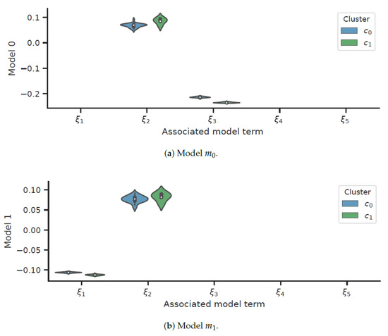
Figure 1.
Coefficient magnitudes for low order SINDyc models.
Model was correctly associated with nonlinear dynamics, and Model was correctly associated with linear dynamics. This only held when choosing a well-posed excitation sequence. The convergence of the SINDyc algorithm was assured only when the identified model was sparse in its coefficients. Consequently, the examination of the sparsity of the identified model provided information on the success of the identification. The uncertainty in the parameters was higher for cluster , in which we had access to only five system observation sequences.
The SINDyc model of the first PR approximates the true system for both the identification data and when considering an out-of-sample experiment. See Figure 2. This works in a similar manner for Model and also for the second cluster . Notice that the design of the out-of-sample excitation signal, in relation to the Sys-ID excitation signal, is an important step to assess the flexibility of the model in describing the true system. We can visually examine the quality of the fit by comparing the one-step prediction surfaces of both the true system and the deduced model. See Figure 3.
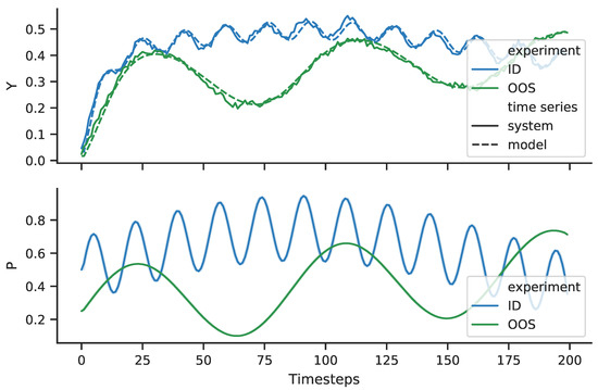
Figure 2.
System response and fitted model response (Y–space) excited by the excitation signal P. Identification experiment ID and out-of-sample experiment OOS.
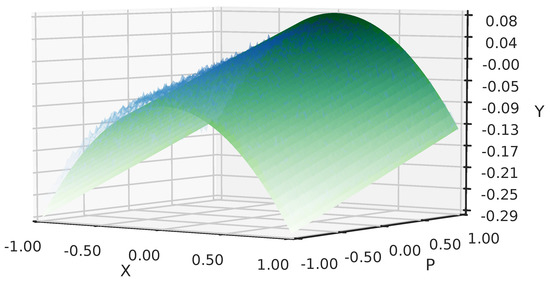
Figure 3.
One-step prediction comparison of the test system (blue) and fitted model (green).
3.2. Model Coefficient Distribution Inference Using MCMC
We now aimed to obtain a probabilistic dynamic system model of the first prosumer based on the identified candidate Model depicted in Figure 1.
At least a subset of the observations in cluster resulted in feasible candidates models, which may inform the prior PDF of the probabilistic model. We may neglect all zero-terms in the candidate model structure in (8) such that the inference through MCMC used only the candidate model as stated in (8). This reduced the computational burden in MCMC. As stated previously, MCMC can handle more complicated prior PDF formulations. The modeler can state more complicated priors based on available system knowledge. For the sake of simplicity, we used Gaussian priors in the exemplary prior PDF stated below.
3.2.1. An Exemplary Prior PDF
We may describe the observation z through the model output y with normally distributed measurement error with variance , corresponding to the measurement equation of the true system stated in (6b):
A log-normal distribution for may be reasonable, such that the mean is . Assuming a constant measurement noise magnitude, we could hereby choose the logarithm of the variance of the observations in the burn-in period. Notice that for the parameter values chosen here, the Gaussian prior model for is appropriate. However, for some prior of , it can be appropriate to use the natural conjugated prior, the inverse Gamma distribution. See [36] for examples.
We assumed the prior for the model coefficients to be normally distributed around , the coefficients inferred using the SINDyc algorithm:
The lack of information in the formulation of this prior we may express through statements of weakly informative priors; see [35] for examples. Furthermore, we considered the following PPC for the evaluation of the accuracy of the inference:
3.2.2. Probabilistic Model
Stan solved the ODE considered here using a Runge–Kutta-45 method. For MCMC, we chose iterations per chain, chains, burn-in or warm-up iterations, no thinning, and a seed specified as . See the parameter values in Table A1, and consider also [31] in this regard.
As the kernel density estimation bandwidth, we used Scott’s rule as given in [37]. The approximated posterior distributions are depicted in Figure 4a alongside the true parameter distributions and the parameter mean inferred by SINDyc. We can observe that the inferred parametric uncertainty was comparably reduced in cluster (see Figure 4a) in comparison to cluster (see Figure 4b). The posterior PDF deviated from the true system’s parametric distributions. Hereby, the parametric mean of the SINDyc models provided a higher precision with respect to the true system’s parametric mean than the inferred parameters.
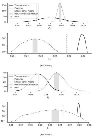
Figure 4.
Inferred coefficient uncertainties through MCMC (posterior PDF) provided a candidate model derived using SINDyc and system observation sequences. Dotted lines mark the prior means based on the chosen SINDyc models. The maximum of the posterior distribution (MAP) is marked. The 95% confidence interval is marked using the shaded area.
Improving the prior optimizes the sampling space for a new MCMC sampling. This can lead to shorter computation time for future sampling of the model. Examining the PPC illustrated in Figure 5a reveals that the model approximated the observed output sub-optimally, yet captured the general trend in the data. By means of random draws from the posterior samples, we could obtain a probabilistic model. Out-of-sample co-simulation of this model alongside the five samples of the true system is depicted in Figure 6.
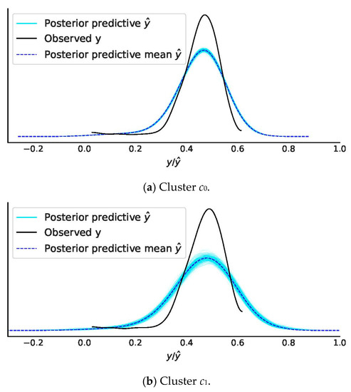
Figure 5.
Posterior predictive check of the model output prediction with 200 samples drawn from the posterior distribution. The plot was generated using the ArviZ library [38].
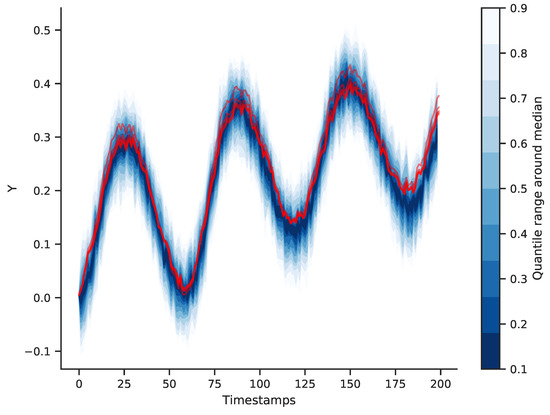
Figure 6.
Out-of-sample simulation of five system realizations and the inferred Stan model (cluster ).
4. Discussion
Activation of system flexibility through DR and PR schemes such as ICo is increasingly relevant in relation to power system operation. See [39] for an example.
Bayesian approaches are computationally complex [26]. The combination of sparse system identification algorithms such as the SINDyc algorithm and MCMC facilitate the inference of model parameters alongside parameter probability estimates. As shown in the related publications [26,27,28], Bayesian inference techniques may benefit from sparsity, promoting modeling approaches. The focus on a viable candidate model and associated parameter spaces reduces the problem size. Aside from this, parsimonious candidate model can be a desirable goal in the modeling process [13].
Similarly, as described in [27], SINDyc models may provide information on whether nonlinearities are present in the data. This works when the algorithm is provided with informative data and a reasonable library of candidate models. Contrary to [27], we coupled the SINDyc algorithm with MCMC in order to obtain a prior PDF that could reduce the computational burden. Automatized Sys-ID pipelines could benefit from such information.
We designed the excitation sequence in the Sys-ID experiment naively by evaluation of the sparsity of the derived SINDyc models. Due to the fact that such experiments must, at least partly, take place during regular system operation, the modeler may consider active learning techniques. Then, the excitation sequence can be designed such that also operational requirements are accounted for. See [40] for an example. Similarly important as the design of the Sys-ID experiment is the design of out-of-sample simulations for evaluation purposes in order to evaluate the model against the true system.
We chose the SINDyc models based on the evaluation of the combined parametric likelihood. The single candidate model then provided the basis for the formulation of the prior PDF. As depicted in Figure 4, the chosen SINDyc parametric mean values introduced a loss in precision with respect to the true mean values. This was a realistic assumption, due to the fact that the true parametric distributions are unknown in the real setting. Similarly, the inferred parametric posterior PDF were sub-optimal with respect to the true distributions.
Hereby, the parametric mean of the SINDyc models provided a higher precision with respect to the true system’s parametric mean than the inferred parameters. In conjunction with the PPC depicted in Figure 5, this may point towards a sub-optimal prior formulation. Furthermore, the polynomial excitation model of third order led to a loss of precision. See Section 2.4 (excitation model).
5. Materials and Methods
The code used to generate the results presented in this paper can be obtained through the following public repository: https://lab.compute.dtu.dk/freba/sindyc-and-mcmc-framework.
6. Conclusions
In this paper, we presented a combination of the SINDyc algorithm and MCMC in the context of PR estimation. While SINDyc identifies sparse and potentially nonlinear dynamical system models, MCMC enables the estimation of potentially complex posterior distributions. MCMC can hereby use a sparse system model identified using SINDyc. Due to the fact that sampling is in this manner performed on a constrained and well-posed sampling space, convergence in MCMC benefits from parsimonious models, and the computational load may be reduced. SINDyc may yield such models, provided the appropriate formulation of the system identification experiment and parameterization of the algorithm. Probabilistic dynamical system models enable the application of SMPC, a core ingredient when aiming to activate prosumer dynamics based on informative grounds.
For future improvements, we may replace the polynomial excitation model described in Section 2.4 with an alternative candidate model structure. Alternatively, we may design the Sys-ID experiment such that we can represent the excitation sequence with the low-order polynomial excitation model described herein. In any case, the objective along these lines is to achieve a high accuracy representation of the excitation signal while maintaining a high performance of the sampling process within the MCMC framework. Furthermore, the combination of SINDyc and MCMC should be evaluated on a broad range of modeling problems. When aiming for automatized Sys-ID, robustness and associated issues are to be investigated and potential solutions to be examined.
Author Contributions
Conceptualization, F.B.; data curation, F.B.; formal analysis, F.B., H.M., N.K.P., and D.G.; funding acquisition, H.M. and N.K.P.; investigation, F.B.; methodology, F.B.; project administration, N.K.P.; resources, F.B., H.M., and N.K.P.; software, F.B.; supervision, N.K.P.; validation, F.B., H.M., and N.K.P.; visualization, F.B.; writing, original draft, F.B.; writing, review and editing, F.B., H.M., and D.G. All authors read and agreed to the published version of the manuscript.
Funding
This work was supported by Innovation Fund Denmark through the CITIES research center (No. 1035-0027B) and by ENERGINET.DK under the project microgrid positioning – uGRIP (No. 77731).
Conflicts of Interest
The authors declare no conflict of interest.
Nomenclature
| Algorithmic Symbols | |
| count_nonzeros | Count nonzeros in |
| count_values | Count values in |
| evaluation_function | Model evaluation function |
| MCMC_function | Function performing MCMC |
| MCMC_params | Parameters to MCMC_function |
| nnz | Number of non-zeros in |
| nval | Number of values in |
| select_Xistar_function | Function selecting from the set of candidate models XI |
| SINDyc_params | Arguments passed to the SINDyc algorithm |
| sparsity_threshold | Permissible fraction of nonzero elements in |
| XI | List of candidate models |
| Mathematical Symbols | |
| Regularization coefficient | |
| Free system dynamics | |
| Set of regularization coefficients | |
| Forced system dynamics | |
| Prior of residual error | |
| Prior of sparse model coefficients | |
| Sparse candidate model coefficients | |
| Posterior predictive check of the system observations z | |
| Prior mean of residual error | |
| Prior dispersion of the residual error | |
| Prior dispersion of candidate model coefficients | |
| Model structure | |
| Prior of the residual error | |
| Posterior distribution of sparse model coefficients | |
| MCMC seed | |
| Sparse model coefficients | |
| model coefficient | |
| b | Sweep bounds |
| Cluster 0, Cluster 1 | |
| Model 0, Model 1 | |
| f | Nonlinear function |
| m | Probabilistic model prior |
| N | Number of observations |
| n | Node n |
| Number of candidate regularization coefficients | |
| Burn-in iterations (warm-up) | |
| Numbers of chains | |
| Iterations per chain | |
| Cluster 0, Cluster 1 | |
| P | Prosumer price response |
| p | Price offer |
| Excitation signal | |
| Sampling rate | |
| v | Measurement noise |
| X | Sys-ID data (system observations) |
| x | System states |
| y | Model output |
| z | System observations |
Abbreviations
The following abbreviations are used in this manuscript:
| DR | demand response |
| EV | electric vehicle |
| ICo | indirect control |
| LASSO | least absolute shrinkage and selection operator |
| MCMC | Markov-chain Monte-Carlo |
| MLE | maximum likelihood estimation |
| NUTS | no-u-turn sampler |
| ODE | ordinary differential equation |
| probability density function | |
| PPC | posterior predictive check |
| PR | prosumer response |
| RES | renewable energy source |
| SINDy | sparse system identification of nonlinear dynamics |
| SINDyc | sparse system identification of nonlinear dynamics with control |
| SMPC | stochastic model predictive controller |
| Sys-ID | system identification |
| V2G | vehicle-to-grid |
Appendix A

Table A1.
Scenario parameterization.
Table A1.
Scenario parameterization.
| Symbol | Relation | Distribution |
|---|---|---|
| ∼ | ||
| ∼ | ||
| ∼ | ||
| v | ∼ | |
| ∼ | ||
| ∼ | ||
| Symbol | Relation | Value |
| = | 1s | |
| = | 50 | |
| = | 5 | |
| = | 100 | |
| b | = | |
| = | 1000 | |
| = | 4 | |
| = | 500 | |
| = | 101 |
References
- Haring, T.; Andersson, G. Contract Design for Demand Response. In Proceedings of the IEEE PES Innovative Smart Grid Technologies, Europe, Istanbul, Turkey, 12–15 October 2014; pp. 1–6. [Google Scholar] [CrossRef]
- Junker, R.G.n.; Azar, A.G.; Lopes, R.A.; Lindberg, K.B.; Reynders, G.; Relan, R.; Madsen, H. Characterizing the Energy Flexibility of Buildings and Districts. Appl. Energy 2018, 225, 175–182. [Google Scholar] [CrossRef]
- Flocha, C.L.; Bellettib, F.; Saxenac, S.; Bayena, R.M.; Mouraa, S. Distributed Optimal Charging of Electric Vehicles for Demand Response and Load Shaping. In Proceedings of the 54th IEEE Conference on Decision and Control, CDC 2015, Osaka, Japan, 15–18 December 2015; p. 7403254. [Google Scholar] [CrossRef]
- Jin, M.; Feng, W.; Liu, P.; Marnay, C.; Spanos, C. MOD-DR: Microgrid Optimal Dispatch with Demand Response. Appl. Energy 2017, 187, 758–776. [Google Scholar] [CrossRef]
- Nwulu, N.I.; Xia, X. Optimal Dispatch for a Microgrid Incorporating Renewables and Demand Response. Renew. Energy 2017, 101, 16–28. [Google Scholar] [CrossRef]
- Sokoler, L.E.; Edlund, K.; Frison, G.; Skajaa, A.; Jø rgensen, J.B. Real-Time Optimization for Economic Model Predictive Control. In Proceedings of the 10th European Workshop on Advanced Control and Diagnosis, Copenhagen, Denmark, 8–9 November 2012. [Google Scholar]
- Short, J.A.; Infield, D.G.; Freris, L.L. Stabilization of Grid Frequency Through Dynamic Demand Control. IEEE Trans. Power Syst. 2007, 22, 1284–1293. [Google Scholar] [CrossRef]
- Ljung, L. System Identification: Theory for the User; Prentice Hall Information and System Sciences Series; Prentice Hall PTR: Upper Saddle River, NJ, USA, 1999. [Google Scholar]
- Nelles, O. Nonlinear System Identification; Springer: Berlin/Heidelberg, Germany, 2001. [Google Scholar] [CrossRef]
- Nguyen, N.T. Model-Reference Adaptive Control; Springer: New York, NY, USA, 2017. [Google Scholar]
- Brunton, S.L.; Proctor, J.L.; Kutz, J.N. Sparse Identification of Nonlinear Dynamics with Control (SINDYc). arXiv 2016, arXiv:1605.06682. [Google Scholar]
- Tibshirani, R. Regression Shrinkage and Selection via the Lasso. J. R. Stat. Soc. Ser. B (Methodol.) 1996, 58, 267–288. [Google Scholar] [CrossRef]
- Brunton, S.L.; Proctor, J.L.; Kutz, J.N. Discovering Governing Equations from Data by Sparse Identification of Nonlinear Dynamical Systems. Proc. Natl. Acad. Sci. USA 2016, 113, 3932–3937. [Google Scholar] [CrossRef]
- Kaiser, E.; Kutz, J.N.; Brunton, S.L. Sparse Identification of Nonlinear Dynamics for Model Predictive Control in the Low-Data Limit. Proc. R. Soc. A 2018, 474. [Google Scholar] [CrossRef]
- De Zotti, G.; Pourmousavi, S.A.; Madsen, H.; Kjolstad Poulsen, N. Ancillary Services 4.0: A Top-to-Bottom Control-Based Approach for Solving Ancillary Services Problems in Smart Grids. IEEE Access 2018, 6, 11694–11706. [Google Scholar] [CrossRef]
- Knudsen, M.D.; Rotger-Griful, S. Combined Price and Event-Based Demand Response Using Two-Stage Model Predictive Control. In Proceedings of the 2015 IEEE International Conference on Smart Grid Communications (SmartGridComm), Miami, FL, USA, 2–5 November 2015; pp. 344–349. [Google Scholar]
- Corradi, O.; Ochsenfeld, H.; Madsen, H.; Pinson, P. Controlling Electricity Consumption by Forecasting Its Response to Varying Prices. IEEE Trans. Power Syst. 2013, 28, 421–429. [Google Scholar] [CrossRef]
- Halvgaard, R.; Poulsen, N.K.L.; Madsen, H.; Jø rgensen, J.B. Economic Model Predictive Control for Building Climate Control in a Smart Grid. In Proceedings of the 2012 IEEE PES Innovative Smart Grid Technologies (ISGT), Washington, DC, USA, 16–20 January 2012; pp. 1–6. [Google Scholar]
- Halvgaard, R.; Poulsen, N.K.; Madsen, H.; Jø rgensen, J.B. Thermal Storage Power Balancing with Model Predictive Control. In Proceedings of the 2013 European Control Conference (ECC), Zurich, Switzerland, 17–19 July 2013; pp. 2567–2572. [Google Scholar]
- Morales, J.M.; Conejo, A.J.; Madsen, H.; Pinson, P.; Zugno, M. Integrating Renewables in Electricity Markets; International Series in Operations Research & Management Science; Springer: Boston, MA, USA, 2014; Volume 205. [Google Scholar] [CrossRef]
- Roscoe, A.; Ault, G. Supporting High Penetrations of Renewable Generation via Implementation of Real-Time Electricity Pricing and Demand Response. IET Renew. Power Gener. 2010, 4, 369. [Google Scholar] [CrossRef]
- Madsen, H.; Parvizi, J.; Halvgaard, R.; Sokoler, L.E.; Jø rgensen, J.B.; Hansen, L.H.; Hilger, K.B. Control of Electricity Loads in Future Electric Energy Systems. In Handbook of Clean Energy Systems; Wiley: Copenhagen, Denmark, 2014; Volume 6, pp. 2213–2236. [Google Scholar]
- Mathieu, J.L.; Vayá, M.G.; Andersson, G. Uncertainty in the Flexibility of Aggregations of Demand Response Resources. In Proceedings of the IECON 2013—39th Annual Conference of the IEEE Industrial Electronics Society, Vienna, Austria, 10–13 November 2013; pp. 8052–8057. [Google Scholar] [CrossRef]
- Bruninx, K.; Pandžic, H.; Cadre, H.L.; Delarue, E. On Controllability of Demand Response Resources Amp; Aggregators’ Bidding Strategies. In Proceedings of the 2018 Power Systems Computation Conference (PSCC), Dublin, Ireland, 11–15 June 2018; pp. 1–7. [Google Scholar] [CrossRef]
- Millar, R.J.; Ekström, J.; Lehtonen, M.; Saarijärvi, E.; Degefa, M.; Koivisto, M. Probabilistic Prosumer Node Modeling for Estimating Planning Parameters in Distribution Networks with Renewable Energy Sources. In Proceedings of the 2017 IEEE 58th International Scientific Conference on Power and Electrical Engineering of Riga Technical University (RTUCON), Riga, Latvia, 12–13 October 2017; pp. 1–8. [Google Scholar] [CrossRef]
- Frigola, R.; Lindsten, F.; Schön, T.B.; Rasmussen, C.E. Bayesian Inference and Learning in Gaussian Process State-Space Models with Particle MCMC. arXiv 2013, arXiv:1306.2861. [Google Scholar]
- Fuentes, R.; Dervilis, N.; Worden, K.; Cross, E. Efficient Parameter Identification and Model Selection in Nonlinear Dynamical Systems via Sparse Bayesian Learning. J. Phys. Conf. Ser. 2019, 1264, 012050. [Google Scholar] [CrossRef]
- Zeng, L.; Shi, L.; Zhang, D.; Wu, L. A Sparse Grid Based Bayesian Method for Contaminant Source Identification. Adv. Water Resour. 2012, 37, 1–9. [Google Scholar] [CrossRef]
- Hirose, K.; Imada, M. Sparse Factor Regression via Penalized Maximum Likelihood Estimation. Stat. Pap. 2018, 59, 633–662. [Google Scholar] [CrossRef]
- Banerjee, O.; Ghaoui, L.E.; d’Aspremont, A. Model Selection Through Sparse Maximum Likelihood Estimation. arXiv 2007, arXiv:0707.0704. [Google Scholar]
- Carpenter, B.; Lee, D.; Brubaker, M.A.; Riddell, A.; Gelman, A.; Goodrich, B.; Guo, J.; Hoffman, M.; Betancourt, M.; Li, P. Stan: A Probabilistic Programming Language. J. Stat. Softw. 2017, 76. [Google Scholar] [CrossRef]
- Hoffman, M.D.; Gelman, A. The No-U-Turn Sampler: Adaptively Setting Path Lengths in Hamiltonian Monte Carlo. J. Mach. Learn. Res. 2014, 15, 1593–1623. [Google Scholar]
- Schmid, P.J. Dynamic Mode Decomposition of Numerical and Experimental Data. J. Fluid Mech. 2010, 656, 5–28. [Google Scholar] [CrossRef]
- Schmid, P.J. Applications of the Dynamic Mode Decomposition. Theor. Comput. Fluid Dyn. 2011, 25, 249–259. [Google Scholar] [CrossRef]
- Gabry, J.; Simpson, D.; Vehtari, A.; Betancourt, M.; Gelman, A. Visualization in Bayesian Workflow. J. R. Stat. Soc. Ser. A (Stat. Soc.) 2019, 182, 389–402. [Google Scholar] [CrossRef]
- Madsen, H.; Thyregod, P. Introduction to General and Generalized Linear Models; Texts in Statistical Science; Chapman & Hall: London, UK, 2010. [Google Scholar]
- Scott, D. Multivariate Density Estimation: Theory, Practice, and Visualization; Wiley Series in Probability and Statistics; Wiley: Hoboken, NJ, USA, 2015. [Google Scholar]
- Kumar, R.; Carroll, C.; Hartikainen, A.; Martin, O. ArviZ a Unified Library for Exploratory Analysis of Bayesian Models in Python. J. Open Source Softw. 2019, 4, 1143. [Google Scholar] [CrossRef]
- Oldewurtel, F.; Roald, L.; Andersson, G.; Tomlin, C. Adaptively Constrained Stochastic Model Predictive Control Applied to Security Constrained Optimal Power Flow. In Proceedings of the 2015 American Control Conference (ACC), Chicago, IL, USA, 1–3 July 2015; pp. 931–936. [Google Scholar] [CrossRef]
- Heirung, T.A.N.; Paulson, J.A.; Lee, S.; Mesbah, A. Model Predictive Control with Active Learning under Model Uncertainty: Why, When, and How. AIChE J. 2018, 64, 3071–3081. [Google Scholar] [CrossRef]
© 2020 by the authors. Licensee MDPI, Basel, Switzerland. This article is an open access article distributed under the terms and conditions of the Creative Commons Attribution (CC BY) license (http://creativecommons.org/licenses/by/4.0/).