Underwater Noise Emission Due to Offshore Pile Installation: A Review

Abstract

The growing demand for renewable energy supply stimulates a drastic increase in the deployment rate of offshore wind energy. Offshore wind power generators are usually supported by large foundation piles that are driven into the seabed with hydraulic impact hammers or vibratory devices. The pile installation process, which is key to the construction of every new wind farm, is hindered by a serious by-product: the underwater noise pollution. This paper presents a comprehensive review of the state-of-the-art computational methods to predict the underwater noise emission by the installation of foundation piles offshore including the available noise mitigation strategies. Future challenges in the field are identified under the prism of the ever-increasing size of wind turbines and the emerging pile driving technologies.

1. Introduction

Driven by the ambitious climate goals to reduce greenhouse gas emissions, the demand for energy generated by wind turbines increased in the past decades [1,2,3,4,5,6]. Offshore wind power generators, in contrast to their onshore counterparts, tend to generate more electricity, as the wind offshore is less turbulent and flows at higher speeds [7]. Nowadays, several foundation concepts exist in offshore wind such as monopiles, tripods, steel jackets, suction caissons and gravity-based foundations [8,9,10]. The choice of the most appropriate concept is governed by several factors like the water depth, the seabed conditions, the expected sea wave heights and the presence of currents and other loads at the location of interest [11,12,13]. Despite the plethora of available concepts, the monopile is the most widely applied foundation type for wind turbines installed in relatively shallow waters with a share of ~75% in the European market alone [14].

Monopiles are driven into the seabed with either hydraulic impact hammers or large vibratory devices as shown in Figure 1 [15]. During impact piling, the hammer delivers a series of short duration pulses at the pile head, forcing the latter into the seabed. In contrast, when vibratory devices are used, the pile is forced gradually into the soil by introducing a quasi-periodic excitation at the pile head [16,17,18]. Regardless of the installation method chosen, noise is generated in the seawater and elastic waves radiate into the seabed. The characteristics of the radiated wave field relate strongly to the method of installation, the pile size and the local site conditions [19]. These elements are key to understanding the noise pollution and the uncertainty in the propagation of the sound field at large distances [20].

Next to the modelling efforts to quantify the noise levels in the seawater, which will be analysed in great detail in this work, many studies focus on the impact of anthropogenic noise emissions on the aquatic species [21,22,23,24]. In impact piling, each strike of the hydraulic hammer generates strong impulsive sound waves in the seawater which propagate at large distance from the construction site [25,26,27,28,29]. The responses of marine mammals and fish to the noise ranges from light disturbance to strong avoidance of the construction site; in extreme cases, even permanent hearing impairment is possible [30,31,32,33,34,35]. The extent of auditory damage depends upon several parameters, i.e., the principal frequency content of the radiated sound, the duration of exposure to high noise levels and the auditory characteristics of the species [36,37,38,39]. Moreover, due to the fact that pile driving activities extend for periods of months, the level of response may also change over time as a result of habituation [40,41,42,43,44].

The underwater sound emission when piles are installed with vibratory devices is less thoroughly explored. The reasons for this are, most likely, attributed to the fact that noise is less severe when compared to impact piling and vibratory methods of installation are less frequently applied offshore. However, a few studies do exist which try to quantify the noise levels [45,46] and assess the environmental impact [47,48]. Even scarcer are studies which investigate systematically the behavioural response of marine mammals when noise mitigation systems are employed [49,50].

The high noise levels generated by offshore construction activities have drawn the attention of regulatory authorities in several nations [51,52,53,54]. Noise assessment reports are nowadays a standard practice prior to the authorisation of a new offshore wind plant [55]. The German Federal government sets specific requirements on the maximum sound levels allowed: 160 dB for the sound exposure level and 190 dB for the sound peak pressure level. Both values are being measured at 750 m from the pile and referenced to ${10}^{-6}$ Pascal [56,57]. In The Netherlands, regulations have recently changed from the allowance of piling during specific period of the year to the adoption of specific sound level criteria [58,59]. The latter are similar to those imposed in Germany, but consider additionally cumulative noise exposure levels. In the United Kingdom, a separate environmental impact assessment (EIA) is followed per project in which acoustic deterrent devices (seal scarers) are used [60] together with trained marine mammal observers who monitor the activity using both visual inspection of the site and passive acoustic detection devices [61,62]. Similar regulations exist in several other countries and lessons learned from previously gathered experiences slowly find their way into new regulations [63,64]. The majority of the regulations though do not consider in detail the frequency content of the radiated noise; an item worth further investigation in the near future [65,66].

This paper reviews the state-of-the-art computational methods to prognosticate the emitted underwater sound during offshore pile installation including the available methods to mitigate the noise. In Section 2, the historical development of the models is presented together with the physics of the sound radiation during pile installation. This serves as a basis for the appreciation of the various modelling efforts and their inherent limitations. Section 3 covers the state-of-the-art in modelling noise due to impact piling. Section 4 presents results of numerical computations for some realistic cases in order to illustrate the importance of some key features for the control of the noise paths. In Section 5, noise mitigation techniques and modelling are reviewed. Finally, Section 6 concludes with the future challenges in the area of noise prediction and mitigation.

2. Structure-Borne Noise in Offshore Piling: The Historical Development of Models

The prediction of underwater noise requires an in-depth study of the source and of the domain in which the acoustic energy is released [67]. Underwater noise in deep oceans is well documented in the literature [68,69,70], driven partly by the need to design SOund Navigation And Ranging (sonar) systems for military applications [71,72]. On the contrary, sound propagation in shallow waters is more complicated due to multiple reflections, refractions and scattering of sound waves at the sea surface and the seabed [73,74,75,76]. The seabed plays a key role here as it is the element that contains the largest uncertainty in the characterisation of its composition [77,78,79].

Next to the challenges associated with wave propagation in shallow waters, the study of noise generated by pile driving, adds an extra complexity; the need to investigate a system composed of three interrelated domains being the seawater, the seabed and the pile, the interaction of which determines the sound source mechanism. Henceforth, a historical overview of the developments in the field of pile vibroacoustics is given, reflecting the evolution of our understanding of the physics of underwater noise emission due to pile driving. This discussion serves as a basis for the understanding of the state-of-the-art models presented in Section 3.

2.1. First Generation Models: The Fluid Approximation of the Seabed

Although some early studies dealing with pile driving noise do exist [80,81,82], Reinhall and Dahl [83] were the first to develop a detailed numerical model focusing on the prediction of underwater noise from impact pile driving. Their approach tackles the problem in two steps: First, a finite element model (FEM) is adopted for the sound generation which includes a sufficient degree of detailing in modelling the source mechanism. Thereafter, the parabolic equation (PE) is applied for the propagation of sound at larger distances [84]. The pile is modelled using structural elements whereas both water and soil are described as linear acoustic fluids. Perfectly Matched Layers (PML) [85] are employed to truncate the fluid domains in the FEM as shown in Figure 2.

The significant result obtained from this study was the observation that the pressure field in the pile proximity is composed of Mach cones, i.e., coherent wave fronts defining alternating zones of compression and rarefaction in the seawater (Figure 2). These are generated by the supersonic compressional stress waves propagating from the pile head to the pile toe right after the hammer impact. Reverse Mach cones were also computed upon reflection of the stress waves from the pile toe. The angle of the cones is equal to ${sin}^{-1}(c_w/c_p)$ ≈ 17.2° in the seawater and ${sin}^{-1}(c_L/c_p)$ ≈ 18.6° in the seabed, with $c_p$, $c_w$ and $c_L$ being the phase speeds of compressional waves in the pile, water, and seabed, respectively. The physics involved mark essentially a moving source problem which is classical in many field of wave mechanics, i.e., supersonic jets [86] or trains that surpass the speed of Rayleigh waves [87,88]. In the case of pile driving, the stress wave in the pile constitutes the moving source. These observations were soon after confirmed by beam forming analysis of measured data [89,90].

The modelling approach introduced by Reinhall and Dahl [83] was subsequently adopted by other researchers [91,92,93,94,95,96,97], i.e., a FEM was employed for the sound generation and a propagation algorithm was applied for wave field predictions at larger distances. As an alternative to the FEM, MacGillivray [98,99,100] adopted a finite difference (FD) scheme for the near-field acoustics under the simplifying assumption of no bending energy stored in the shell surface. Depending on the degree of detailing required, the far-range propagation model can take several mathematical forms:

• normal mode (NM) representations [97],
• wavenumber intergation (WI) algorithms [91,93,94],
• energy flux-based methods [101] and
• parabolic equation (PE) models [83,96,102,103].

Numerical models which couple the structural domain modelled by finite elements and the exterior (soil) domain modelled by means of the boundary element method also exist [104,105,106], albeit their focus is primarily placed on the soil vibrations in the pile proximity.

In contrast to the models described above, which are primarily based on numerical discretisation of the partial differential equations, semi-analytical solutions were also proposed by several authors [107,108,109,110,111,112]. The analytical model by Hall [110] considers a thin cylindrical shell immersed in a fluid in which semi-analytical solutions are obtained for the radiated sound pressure and particle velocity similar to Junger and Feit [113].

In the model by Tsouvalas and Metrikine [107] (Figure 3), the pile is modelled using the shell theory, the water is described as a linearised acoustic fluid and the soil is treated by distributed springs and dashpots attached to the pile surface. The shell and water responses are expressed in terms of modes and then a mode matching technique is employed to solve the coupled problem. The models by Deng et al. [111], Deng et al. [112] are similar to those in [107], but expand the shell response in terms of different basis functions. The advantage of the semi-analytical models is that they are computationally fast and can be used when a large number of simulations are required. The downside of this is that they are not able to achieve the same degree of detailing as in FEM.

2.2. Second Generation Models: Inclusion of the Elastic Seabed

The models described in Section 2.1 constitute a significant step towards understanding the physics of underwater sound emission in impact piling. However, their main limitation is that they describe the seabed either by an acoustic medium or by spring-dashpot elements. The former approximation, albeit reasonable in many ocean acoustic applications, cannot capture all the essential physics of the problem at hand for two main reasons. First, the energy is largely released in the seabed during pile driving while the pile is partly embedded into the soil [114]. Thus, an accurate prediction of the energy flux in the surrounding acousto-elastic region requires a detailed description of the seabed next to that of the seawater. Second, the accurate identification of the acoustic source amplitude, i.e., pile response, requires the consideration of the coupled soil–fluid–pile problem. In other words, without an accurate description of the coupled problem, the noise source mechanism cannot be identified properly.

Tsouvalas et al. [115,116,117,118] were among the first to include the elastic description of the seabed in the pile driving acoustics. In Figure 4, results of model simulations are shown for illustration of the physics of the wave radiation pattern for a typical case of an offshore pile installation scenario. Next to the pressure cones in the seawater, the response in the soil is dominated by shear waves with almost vertical polarisation because the shock waves in the pile travel at hypersonic speed compared to that of the shear waves in the soil ($M=c_p/c_S\approx 27$). Additionally, compressional waves exist in the seabed similar to the ones observed in the seawater. Apart from the waves travelling in the bulk of the media, Scholte waves are generated at the seabed–water interface travelling with much lower speed compared to the speed of the compressional waves. The prediction of these elastic waves was later confirmed by several authors [119,120,121,122,123], while experimental data measuring the soil response together with the pressures in the water column close to the seabed have confirmed the existence of the interface waves [124,125].

3. The State-Of-The-Art in Predictive Modelling of Sound

While Section 2 focused primarily on the explanation of the physics of the waves radiated in the seabed and the water column during impact piling, this section reviews the available modelling techniques in greater depth including the mathematical statement of the vibroacoustic problem and the available methods to solve the coupled system of partial differential equations. Acoustic models can be categorised into groups based on the degree of detail in modelling the sound source and the domain in which the energy is released. Given this categorisation, models can span a whole range from empirical ones to very detailed numerical ones.

Section 3.1 discusses the state-of-the-art empirical models to estimate sound levels in the case of impact piling. Section 3.2 presents the set governing equations of the coupled vibroacoustic system which forms the starting point of all advanced modelling efforts. Section 3.3 and Section 3.4 introduce the semi-analytical and the numerical approaches, respectively, employed to solve the mathematical statement of the problem. Finally, Section 3.5 concludes with a concise overview of all models available to date.

3.1. Empirical Models

In empirical models, the acoustic source is described in terms of a sound level without giving a detailed description of its geometry and excitation characteristics. Subsequently, this reference sound level is propagated at larger distances by means of a transmission loss formula which is based on the source–receiver distance and the characteristics of the acoustic domain under consideration. To this end, empirical or semi-empirical formulae are derived on the basis of energy attenuation laws and underwater noise measurements carried out in several environments [126,127,128,129].

Attempts to apply similar methods in impact piling and vibratory installation have also been reported recently [130,131,132,133]. The most recent formula proposed to estimate the (averaged over the depth of the water column) sound exposure level $L_E$ ($L_{E,p}$ according to [134]) from impact piling reads [131]:

$$L_E\left(r\right)=L_E\left(r_1\right)-10{log}_{10}(r/r_1)-\alpha (r-r_1)$$

(1)

In Equation (1), r is the radial distance from the pile, $r_1$ defines the reference range in which the sound level is known and $\alpha$ is a decay factor in [dB m⁻¹]. This marks essentially a damped cylindrical spreading (DCS) model of the form $L_E\left(\overline{r}\right)=\left[\text{source level}\right]-A{log}_{10}\left(\overline{r}\right)-B\overline{r}$, in which $\overline{r}$ defines the source-receiver distance, $A=10$, and the parameter $B=\alpha$ can vary depending on the reflectivity of the seabed and the grazing angle between the Mach cone and seabed. The depth-averaged sound exposure level $L_E$ is defined as [131]

$$L_E=10{log}_{10}\left(\frac{1}{p_0^2{T}_0}\underset{t=t_1}{\overset{t=t_2}{\int }}{p}^2\left(t\right)dt\right)$$

(2)

in which $T_0=1$ s, $p_0={10}^{-6}$ Pa, and the impulsive signal being fully enclosed between the time moments $t_1$ and $t_2$. The physical quantity $p^2\left(t\right)$ corresponds to depth-averaged squared sound pressure from the signal alone, excluding all other sources of acoustic noise [134]. The frequency-independent decay factor $\alpha$ is given as

$$\alpha =\frac{-10{log}_{10}{\left(\right|R|}^2)}{2Hcoth\left(\theta \right)}$$

(3)

The loss at bottom interaction is described in terms of the squared magnitude of the reflection factor R between water and assumed seabed half-space, the angle $\theta$ represents the angle of Mach cone (about 17° as discussed in Section 2.1) and H is the water depth in meters. The main challenge here lies in a reasonable estimation of the $\alpha$-factor which can be approximated by Equation (3); however, this serves only as a first-order estimation. The DCS model proposed by Lippert et al. [131] has been adjusted recently for environments of varying bathymetry and seabed properties by Martin and Barclay [132].

For the estimation of the peak pressure level $\mathrm{S}\mathrm{P}{\mathrm{L}}_{peak}$ a similar formula is proposed that requires as input the $L_E$ and the properties of the hammer strike [130]:

$$\mathrm{S}\mathrm{P}{\mathrm{L}}_{peak}=A{L}_E+B+C\left({\left[\frac{Z_p}{m_r}\right]}_0-{\left[\frac{Z_p}{m_r}\right]}_1\right)$$

(4)

The subscript indices in the squared brackets stand for the site from which the regression coefficients A and B are derived $\left(0\right)$ (empirical constants estimated from measurements) and the unknown site for which the $\mathrm{S}\mathrm{P}{\mathrm{L}}_{peak}$ is to be estimated $\left(1\right)$, with the empirical factor C having the unit [dB s]. Additionally, $m_r$ is the mass of the hammer and $Z_p=E_p{A}_p/c_p$ is the pile impedance [135], with $E_p$ being the Young’s modulus of the pile, $A_p$ its cross-sectional area and $c_p$ the axial wave velocity in the pile.

Equations (1)–(4) are very attractive for a quick prognosis of the noise levels at a given location, especially when the values of the decay factor $\alpha$ in Equation (1), or the coefficients $A,B$ and C in Equation (4), can be estimated with reasonable accuracy. However, their use should be exercised with caution and only when one fully understands their inherent limitations. First, one should be able to obtain the sound level in the pile proximity, i.e., sound level at the source distance $r_1$, which can then be inserted into an empirical model for sound tranmission. Thus, the task of developing a model for the generation of sound still remains. Second, one should feel confident that the estimation of the decay factor $\alpha$ at the location of interest is reasonable. Third, the formulae can only be used to estimate the sound exposure level $L_E$, and possibly the $\mathrm{S}\mathrm{P}{\mathrm{L}}_{peak}$ with some degree of confidence [130]; a complete picture of the sound field cannot be retrieved in this case.

In conclusion, empirical models, although useful at the early stages of design of a project, when pile dimensions are not yet fixed and detailed data are not yet available at the location of interest, are not detailed enough to make a solid statement regarding the sound field which may be required for the design and optimal deployment of noise mitigation systems [136].

3.2. Advanced Models: The Mathematical Statement of the Problem

Most advanced models treat the problem in two steps as illustrated in Figure 5. A close-range module is used to generate the wave field at pile proximity ($r\le r_0$) and this field is subsequently coupled at $r=r_0$ to a far-range module for the propagation of sound at larger distances ($r\ge r_0$). The basic model is cylindrically symmetric and consists of the pile and the surrounding medium, i.e., the seawater column overlying a stack of horizontally stratified elastic layers. In some models, seabed shear rigidity is excluded (Section 2.1). Classical (low-order) shell theories are considered for the description of the pile dynamics [137,138], which suffice in most cases since the excited wavelengths in the structure are a magnitude larger when compared to the shell’s thickness. High-order corrections, accounting for shear deformation and rotatory inertia, are required only in those cases in which the lengths of the excited waves in the shell structure are relatively short, i.e., ${\lambda }_{min}\sim t$ with ${\lambda }_{min}$, t being the shorter wavelength excited and the thickness of the shell, respectively [139].

Let us assume that the pile is of finite length and occupies the domain $0\le z\le L$. The constants R, t, $\nu$ and $\rho$ define the radius, thickness, Poisson’s ratio and density of the shell, respectively. The fluid is modelled as a three-dimensional inviscid compressible medium having a pressure release boundary at $z=z_0$ and occupying the domain $z_0\le z\le z_1$, $r\ge R+t/2$. The seabed is modelled as a three-dimensional elastic continuum which occupies the domain $z_1\le z<\infty$, $r\ge R+t/2$. The constants ${\lambda }_j$, ${\mu }_j$ and ${\rho }_j$ define the $Lam\stackrel{‘}{e}$ coefficients and the density of each solid layer, respectively. The dynamics of the total system are described by the following set of partial differential equations.

$$\mathbf{L}{\mathbf{u}}_p+{\mathbf{I}}_m{\ddot{\mathbf{u}}}_p=-\left(H(z-z_1)-H(z-L)\right){\mathbf{t}}_s+\left(H(z-z_0)-H(z-z_1)\right){\mathbf{p}}_f+\mathbf{f}$$

(5)

$${\mu }_j{\nabla }^2{\mathbf{u}}_s^j+\left({\lambda }_j+{\mu }_j\right)\nabla \nabla ·{\mathbf{u}}_s^j-{\rho }_j{\ddot{\mathbf{u}}}_s^j=\mathbf{0},j=1,2,\dots ,N$$

(6)

$${\nabla }^2{\varphi }_f(r,z,t)-\frac{1}{c_f^2}{\ddot{\varphi }}_f(r,z,t)=0$$

(7)

In Equations (5)–(7), ${\mathbf{u}}_p={\left[u_{p,z}(z,t)u_{p,r}(z,t)\right]}^{\mathrm{T}}$ and ${\mathbf{u}}_s^j(r,z,t)={\left[u_{s,z}^j(r,z,t)u_{s,r}^j(r,z,t)\right]}^{\mathrm{T}}$ are the displacement vectors of the shell and of each solid layer, respectively, and ${\varphi }_f(r,z,t)$ denotes the velocity potential of the fluid. The constant $c_f$ defines the compressional phase speed of waves in the seawater assuming here an isovelocity water column. The operators $\mathbf{L}$ and ${\mathbf{I}}_m$ are based on the chosen shell theory adopted [115]. The vector ${\mathbf{p}}_f$ corresponds to the fluid pressure exerted at the surface of the shell at $z_0<z<z_1$ and $H(z-z_i)$ denote the Heaviside step functions. The vector $\mathbf{f}={\left[f_{rz}(z,t)f_{rr}(z,t)\right]}^T$ represents the externally applied force and ${\mathbf{t}}_s$ represents the boundary stress vector that takes into account the reaction of the soil surrounding the shell at $z_1<z<L$. For each solid layer one obtains

$${\mathbf{t}}_s^j=\left[{\lambda }_j\nabla ·{\mathbf{u}}_s^j\mathbf{I}+{\mu }_j\left(\nabla {\mathbf{u}}_s^j+{\left(\nabla {\mathbf{u}}_s^j\right)}^T\right)\right]·\widehat{\mathbf{r}},$$

(8)

in which ${\mathbf{t}}_s^j$ is the solid stress tensor of layer j, $\widehat{\mathbf{r}}$ is the unit normal vector to the surface of the shell and $\mathbf{I}$ is the identity matrix.

The boundary and interface conditions between the adjacent layers at $r\ge R$ read:

$$p_f(r,z_0,t)=0$$

(9)

$${\sigma }_{s,zz}^1(r,z_1,t)+p_f(r,z_1,t)=0,{\sigma }_{s,zr}^1(r,z_1,t)=0,u_{s,z}^1(r,z_1,t)-u_{f,z}(r,z_1,t)=0$$

(10)

$${\sigma }_{s,zi}^{j+1}(r,z_j,t)-{\sigma }_{s,zi}^j(r,z_j,t)=0,u_{s,i}^{j+1}(r,z_j,t)-u_{s,i}^j(r,z_j,t)=0,2\le j\le n-1,i=z,r$$

(11)

$$u_{s,r}^n(r,H,t)=u_{s,z}^n(r,H,t)=0$$

(12)

In Equations (10) and (11), ${\sigma }_{s,zi}^j$ denotes the stresses in the correspondent layer j. Equation (12) is adopted in [115] to ease the analytical treatment of the problem by introducing a rigid surface at $z=H$ (Figure 5). These equations are substituted by the radiation condition at $z\to \infty$ in the FE models; the latter being materialised in FEM in terms of PMLs [85] or other non-reflecting boundaries. To complete the mathematical statement of the problem, the kinematic continuities at the interfaces of the pile with the water and the soil need to be imposed together with the boundary conditions at $r\to \infty$:

$$u_{p,r}(z,t)-u_{f,r}(R,z,t)=0,z_0<z<z_1$$

(13)

$$u_{p,i}(z,t)-u_{s,i}(R,z,t)=0,z_1<z<L,i=z,r$$

(14)

In Equations (10) and (13), $u_{f,z}(r,z,t)$ and $u_{f,r}(r,z,t)$ correspond to the vertical and radial displacements in the water column, respectively. The radiation conditions at $r\to \infty$ are satisfied either exactly in semi-analytical treatments [107,115] or approximately by employing PMLs [83] in FEMs.

It is important to realise that the mathematical statement of the problem given by the system of coupled partial differential equations (PDEs) (5)–(14) is similar in all available models with only some minor modifications in the boundary/interface conditions or in approximations made for the far-range model (Section 3.4). This is despite the fact that the solution approach may differ significantly between the various methods. Numerical methods employ either finite elements or finite differences to reduce the system of coupled PDEs to a system of ordinary differential equations (ODEs) by means of direct spatial discretisation. Semi-analytical methods usually transform the set of Equations (5)–(14) into the frequency domain first and proceed further with the solution as discussed in Section 3.3.

3.3. Semi-Analytical Solution Methods

With semi-analytical models we refer to those models which reduce the system of PDEs to a system of algebraic equations [107,108,109,110,111,112,115]. Their complexity can vary significantly based on different underlying assumptions. Hereafter, the model introduced in [140] is described in detail as it is the most complete one in this group including a layered elastic seabed.

3.3.1. Close-Range Module

The starting point of the solution approach is a Fourier transform of Equations (5)–(14) into the frequency domain. Subsequently, a modal decomposition is applied both for the shell structure and the acousto-elastic waveguide. The modal expansion of the shell structure (in the frequency domain) reads

$${\tilde{u}}_{p,k}(z,\omega )=\sum _{m=1}^{\infty }{A}_m{U}_{km}\left(z\right)$$

(15)

The index $k=z,r$ indicates the displacement component, $m=1,2,\dots ,\infty$ is the axial order and the vertical eigenfunctions $U_{km}\left(z\right)$ satisfy the boundary conditions at $z=0,L$. The closed form expressions for the displacement and stress fields, which satisfy Equations (9)–(12) as well as the boundary conditions at $r\to \infty$, read [115]

$${\tilde{u}}_{f,z}(r,z,\omega )=\sum _{p=1}^{\infty }{C}_p{H}_0^{\left(2\right)}\left(k_{p}r\right){\tilde{u}}_{f,z,p}\left(z\right),{\tilde{u}}_{f,r}(r,z,\omega )=\sum _{p=1}^{\infty }{C}_p{H}_1^{\left(2\right)}\left(k_{p}r\right){\tilde{u}}_{f,r,p}\left(z\right)$$

(16)

$${\tilde{u}}_{s,r}(r,z,\omega )=\sum _{p=1}^{\infty }{C}_p{H}_1^{\left(2\right)}\left(k_{p}r\right){\tilde{u}}_{s,r,p}\left(z\right),{\tilde{u}}_{s,z}(r,z,\omega )=\sum _{p=1}^{\infty }{C}_p{H}_0^{\left(2\right)}\left(k_{p}r\right){\tilde{u}}_{s,z,p}\left(z\right)$$

(17)

$${\tilde{\sigma }}_{s,zz}(r,z,\omega )=\sum _{p=1}^{\infty }{C}_p{H}_0^{\left(2\right)}\left(k_{p}r\right)\left(k_p{\lambda }_s{\tilde{u}}_{s,r,p}\left(z\right)+{\rho }_s{c}_L^2\frac{d{\tilde{u}}_{s,z,p}\left(z\right)}{dz}\right)$$

(18)

$${\tilde{\sigma }}_{s,zr}(r,z,\omega )=\sum _{p=1}^{\infty }{\mu }_s{C}_p{H}_1^{\left(2\right)}\left(k_{p}r\right)\left(\frac{d{\tilde{u}}_{s,r,p}\left(z\right)}{dz}-k_p{\tilde{u}}_{s,z,p}\left(z\right)\right)$$

(19)

$${\tilde{\sigma }}_{s,rr}(r,z,\omega )=\sum _{p=1}^{\infty }{C}_p\left(H_0^{\left(2\right)}\left(k_{p}r\right){\tilde{\sigma }}_{s,rr,p}^{H_0}\left(z\right)+\frac{1}{r}{H}_1^{\left(2\right)}\left(k_{p}r\right){\tilde{\sigma }}_{s,rr,p}^{H_1}\left(z\right)\right),$$

(20)

$${\tilde{p}}_f(r,z,\omega )=\sum _{p=1}^{\infty }{C}_p{H}_0^{\left(2\right)}\left(k_{p}r\right){\tilde{p}}_{f,p}\left(z\right)$$

(21)

with:

$${\tilde{\sigma }}_{s,rr,p}^{H_0}\left(z\right)=k_p{\rho }_s{c}_L^2{\tilde{u}}_{s,r,p}\left(z\right)+{\lambda }_s\frac{d{\tilde{u}}_{s,z,p}\left(z\right)}{dz}\mathrm{and}{\tilde{\sigma }}_{s,rr,p}^{H_1}\left(z\right)=-2{\mu }_s{\tilde{u}}_{s,r,p}\left(z\right)$$

In Equations (15)–(21), the only unknowns are the modal coefficients $A_m$ and $C_p$ which can be determined by solving the forced response of the complete system. The term $k_p$ denotes the horizontal wavenumber which is the solution of the dispersion equation formed by the set of Equations (9)–(12) while the functions of the $z-$ coordinate entering the infinite summations, i.e., ${\tilde{u}}_{f,i,p}\left(z\right)$ and ${\tilde{u}}_{s,i,p}\left(z\right)$ with $i=z,r$, are vertical eigenfunctions in the acousto-elastic domain of interest.

A system of infinite algebraic equations with respect to the unknown coefficients $C_p$ can be obtained by an appropriate combination of Equations (13) and (14) and the use of Equation (5) [19]:

$$\sum _{q=1}^{\infty }{C}_q\left(L_{qp}+k_q{H}_1^{\left(2\right)}\left(k_{q}R\right){\Gamma }_q{\delta }_{qp}-\sum _{m=1}^{\infty }\frac{R_{mq}{Q}_{mp}}{I_m}\right)=\sum _{m=1}^{\infty }\frac{F_m{Q}_{mp}}{I_m}$$

(22)

The terms $L_{qp}$, ${\Gamma }_q$, $Q_{mp}$, $R_{mp}$, $F_m$ and $I_m$ introduced in Equation (22) are given as [115]

$$L_{qp}=H_1^{\left(2\right)}\left(k_{p}R\right)\underset{z_2}{\overset{L}{\int }}{\tilde{u}}_{s,z,p}\left(z\right){\tilde{\sigma }}_{s,zr,q}\left(z\right)dz-H_0^{\left(2\right)}\left(k_{p}R\right)\underset{z_2}{\overset{L}{\int }}{\tilde{u}}_{s,z,q}\left(z\right)\frac{{\tilde{\sigma }}_{s,zr,p}\left(z\right)}{k_p}dz$$

$$\begin{array}{c}\hfill {\Gamma }_p{\delta }_{pq}=-\underset{z_1}{\overset{z_2}{\int }}\frac{{\tilde{u}}_{f,r,q}\left(z\right)}{k_q}{\tilde{p}}_{f,p}\left(z\right)+\underset{z_2}{\overset{L}{\int }}\left[{\zeta }_s{k}_p^2\frac{{\tilde{u}}_{s,r,p}\left(z\right)}{k_p}\frac{{\tilde{u}}_{s,r,q}\left(z\right)}{k_q}+{\eta }_s\frac{{\tilde{u}}_{s,r,q}\left(z\right)}{k_q}{\tilde{\sigma }}_{s,zz,p}\left(z\right)-{\tilde{u}}_{s,z,p}\left(z\right)\frac{{\tilde{\sigma }}_{s,zr,q}\left(z\right)}{k_q}\right]dz\end{array}$$

$$\begin{array}{c}\hfill Q_{mp}=-\underset{z_1}{\overset{z_2}{\int }}{U}_{rm}{\tilde{p}}_{f,p}dz+\underset{z_2}{\overset{L}{\int }}\left(U_{rm}\left(z\right)\left({\eta }_s{\tilde{\sigma }}_{s,zz,p}\left(z\right)+{\zeta }_s{k}_p{\tilde{u}}_{s,r,p}\left(z\right)\right)+U_{zm}\left(z\right)\frac{{\tilde{\sigma }}_{s,zr,p}\left(z\right)}{k_p}\right)dz\end{array}$$

$$\begin{array}{c}\hfill R_{mp}=H_0^{\left(2\right)}\left(k_{p}R\right)\underset{z_1}{\overset{z_2}{\int }}{U}_{rm}\left(z\right){\tilde{p}}_{f,p}\left(z\right)dz-H_1^{\left(2\right)}\left(k_{p}R\right)\underset{z_2}{\overset{L}{\int }}{U}_{zm}\left(z\right){\tilde{\sigma }}_{s,zr,p}\left(z\right)dz\\ \hfill -H_0^{\left(2\right)}\left(k_{p}R\right)\underset{z_2}{\overset{L}{\int }}{U}_{rm}\left(z\right){\tilde{\sigma }}_{s,rr,p}^{H_0}\left(z\right)dz-H_1^{\left(2\right)}\left(k_{p}R\right)\underset{z_2}{\overset{L}{\int }}{U}_{rm}\left(z\right){\tilde{\sigma }}_{s,rr,p}^{H_1}\left(z\right)dz\end{array}$$

$$F_m=\underset{0}{\overset{L}{\int }}\left(U_{zm}\left(z\right){\tilde{f}}_{zr}\left(z\right)+U_{rm}\left(z\right){\tilde{f}}_{rr}\left(z\right)\right)dz$$

$$I_m=2\rho h\underset{0}{\overset{L}{\int }}\left(U_{zm}^2\left(z\right)+U_{rm}^2\left(z\right)\right)dz\left({\omega }^2-(1+\mathrm{i}\xi ){\omega }_m^2\right)$$

In the integral expressions defined above, ${\omega }_m$ defines the eigenfrequencies of the shell. The parameters ${\zeta }_s={\rho }_s\left(z\right)c_L^{-2}\left(z\right)\left(c_L^4\left(z\right)-{\left(c_L^2\left(z\right)-2c_T^2\left(z\right)\right)}^2\right)$ and ${\eta }_s=c_L^{-2}\left(z\right)\left(c_L^2\left(z\right)-2c_T^2\left(z\right)\right)$ define soil coefficients with $c_L\left(z\right)$ and $c_T\left(z\right)$ being the compressional and shear wave speeds in the soil. These functions depend on the vertical coordinate z, albeit in a piecewise discontinuous manner in the configuration examined here (Figure 5). The factor $\xi$ is the structural loss factor of the steel material [141]. Finally, the coefficients of the shell structure are given by

$$A_m=\frac{F_m+{\displaystyle \sum _{p=1}^{\infty }}{C}_p{R}_{mp}}{I_m}$$

(23)

By following the approach above, the original system of PDEs is reduced to an infinite system of algebraic equations, i.e., Equation (22), provided that the modal expansions over the shell and acousto-elastic modes are properly truncated [142]. Obviously, the treatment here is restricted to a cylindrically symmetric case; however, an extension of the method to treat non-vertical forces is also possible [19].

3.3.2. Far-Range Module

Naturally, the solution described in Section 3.3.1 allows the evaluation of the field at any distance from the pile. However, the presence of a rigid surface at $z=H$, i.e., Equations (12), may lead to spurious wave reflections at large (from the pile) distances which are non-physical. To overcome this problem, the wave field generated at the pile proximity is used as input to a far-range module. The basis of the far-from-source model is the built-up of the Green’s matrix for the acousto-elastic system in which the excitation is a ring source positioned at a given radius and depth (either in the soil or in the fluid) [140].

Let us assume that a ring source is positioned at $r_0$, $z_0$ as shown in Figure 6a. The equations of motion of the shear and compressional potentials of the acousto-elastic domain (in the frequency domain) read

$$[{\nabla }^2+k_{\xi }^2]\tilde{G}(r,z;r_0,z_0,\omega )=\frac{\delta (r-r_0,z-z_0)}{2\pi r}{S}_{\xi }\left(\omega \right)$$

(24)

The delta function $\delta (r-r_0,z-z_0)$ represents the source term [143], while $k_{\xi }$ with index $\xi =f,p_j$ or $s_j$ represent the medium wavenumbers, i.e., $k_f=\omega /c_f,k_{p,j}=\omega /c_{p,j},k_{s,j}=\omega /c_{s,j}$. $S_{\xi }\left(\omega \right)$ represents the source strength in the correspondent layer. Application of the forward Hankel transform to Equation (24) yields

$$\left[\frac{d^2}{d{z}^2}+k_{z,\xi }^2\right]\widehat{G}(k_r,z;r_0,z_0,\omega )=\frac{\delta (z-z_0)}{2\pi }{J}_0\left(k_r{r}_0\right)S_{\xi }\left(\omega \right)$$

(25)

in which $k_{z,\xi }=\sqrt{k_{\xi }^2-k_r^2}$. $\tilde{G}$ and $\widehat{G}$ denote the Green’s functions in frequency and Hankel domains, respectively. Once the solution in the Hankel domain is known, the inverse Hankel transform yields

$$\tilde{G}(\mathit{r};{\mathit{r}}_0,\omega )=-\frac{1}{2}{\int }_{-\infty }^{+\infty }(S_{\xi }\left(\omega \right)\frac{e^{-i{k}_{z,\xi }\mid z-z_0\mid }}{4\pi i{k}_{z,\xi }}+A_{\xi }^1{e}^{i{k}_{z,\xi }z}+A_{\xi }^2{e}^{-i{k}_{z,\xi }z})J_0\left(k_r{r}_0\right)H_0^{\left(2\right)}\left(k_{r}r\right)k_{r}d{k}_r$$

(26)

For $z\ge z_N$, $A_{\xi }^1=0$ to ensure that the out-going waves leave the soil half-space without reflection. Upon substitution of the above solutions into the boundary and interface conditions given by Equations (9)–(11), it is straightforward that the kernels in the integral representations need to be satisfied. This yields a linear algebraic system with unknowns $A_{\xi }^1$ and $A_{\xi }^2$. Once the amplitude coefficients are obtained for every $k_r$, the Green’s tensor for any configuration of compressional or shear (ring) source potentials is known.

To evaluate the wavenumber integral given by Equation (26), the complex contour integration technique is applied. The solution can be expressed as a summation of finite number of (normal) modes supplemented by Ewing–Jardetsky–Press (EJP) branch line integrals [144] (Figure 6b). The characteristic equation $f\left(k_r\right)$, being the determinant of the coefficient matrix, is used to determine the horizontal wavenumbers $k_r^{\left(m\right)}$ (defining the residues’ contribution enclosed by the chosen integration path). The final expression of the Green’s tensor assuming a unit strength source amplitude reads

$$\begin{array}{c}\hfill \tilde{G}(r,z;r_0,z_0,\omega )=-\pi i\sum _{m=1}^{\infty }\frac{{\widehat{G}}^{\star ,num}(k_r^{\left(m\right)},z;z_0)}{f^{\prime }\left(k_r^{\left(m\right)}\right)}{J}_0\left(k_r^{\left(m\right)}{r}_0\right)H_0^{\left(2\right)}\left(k_r^{\left(m\right)}r\right)k_r^{\left(m\right)}\\ \hfill +\frac{1}{2}{\int }_{\alpha +\beta }^{}\widehat{G}(k_r,z;r_0,z_0)J_0\left(k_r{r}_0\right)H_0^{\left(2\right)}\left(k_{r}r\right)k_{r}d{k}_r\end{array}$$

(27)

in which ${\widehat{G}}^{\star ,num}$ denote the numerator of the terms in parentheses of the Green’s function in the Hankel domain and $f^{\prime }\left(k_r^{\left(m\right)}\right)$ denotes the derivative of the characteristic equation. Finally, the Green’s tensor $\tilde{\mathbf{G}}(r,z;r_0,z_0,\omega )$ can be composed from the individual elements by changing subsequently the position of the source and the receiver points in the layered medium.

The direct boundary element method (BEM) is adopted to couple the near-source and far-from-source modules [145,146,147,148]. The boundary data specified from the near-source module on a cylindrical surface at $r=r_0$ (Section 3.3.1), are used as input to the far-from-source module via the BEM. The fundamental solutions of Green’s displacement tensors ${\tilde{U}}_{\alpha \beta }^{\Xi \xi }(\mathit{r},{\mathit{r}}_0,\omega )$ are derived from the potential functions [149] given the receiver point at $\mathit{r}=(r,z)$ (in medium $\Xi$) in $\alpha$-direction due to a unit impulse at source ${\mathit{r}}_0=(r_0,z_0)$ (in medium $\xi$) in $\beta$-direction:

$$\begin{array}{cc}\hfill & {\tilde{U}}_{\alpha \beta }^{s\xi }(\mathit{r},{\mathit{r}}_0,\omega )=\nabla {\tilde{\varphi }}_{s_j,\xi }^g(\mathit{r},{\mathit{r}}_0,\omega )+\nabla \times W,W=-\frac{\partial {\psi }_{s_j,\xi }^g(\mathit{r},{\mathit{r}}_0,\omega )}{\partial r}\hfill \\ \hfill & {\tilde{U}}_{\alpha \beta }^{f\xi }(\mathit{r},{\mathit{r}}_0,\omega )=\nabla {\tilde{\varphi }}_{f,\xi }^g(\mathit{r},{\mathit{r}}_0,\omega )\hfill \end{array}$$

(28)

For the elastic domain, the Green’s stress tensors ${\tilde{T}}_{\alpha \beta }^{\Xi \xi }(\mathit{r},{\mathit{r}}_0,\omega )$ related to ${\tilde{U}}_{\alpha \beta }^{\Xi \xi }(\mathit{r},{\mathit{r}}_0,\omega )$ can be obtained through substitution of Equation (28) into the constitutive equations [149]. The fundamental solution pair {${\tilde{U}}_{\alpha \beta },{\tilde{T}}_{\alpha \beta }$} can be obtained by introducing unit amplitude stress jumps at the plane of the source, i.e., at $z=z_0$ [150]:

$$\begin{array}{cc}\hfill {\tilde{\sigma }}_{zr}(r,z_0^{+},\omega )-{\tilde{\sigma }}_{zr}(r,z_0^{-},\omega )& =\frac{\delta (r-r_0)}{2\pi r}\hfill \\ \hfill {\tilde{\sigma }}_{zz}(r,z_0^{+},\omega )-{\tilde{\sigma }}_{zz}(r,z_0^{-},\omega )& =\frac{\delta (r-r_0)}{2\pi r}\hfill \\ \hfill {\tilde{u}}_r(r,z_0^{+},\omega )-{\tilde{u}}_r(r,z_0^{-},\omega )& =0\hfill \\ \hfill {\tilde{u}}_z(r,z_0^{+},\omega )-{\tilde{u}}_z(r,z_0^{-},\omega )& =0\hfill \end{array}$$

(29)

Owing to the absence of the source in the domain above (at $z_0^{+}<z_0$) and below (at $z_0^{-}>z_0$) the introduced stress jumps, the Green’s potential function can be determined directly by solving for the amplitudes $A_{\xi ,z_0^{+}}^1$, $A_{\xi ,z_0^{-}}^1$, $A_{\xi ,z_0^{+}}^2$ and $A_{\xi ,z_0^{-}}^2$ and by setting $S_{\xi }\left(\omega \right)=0$ ($\xi =p_j,s_j$). For the acoustic domain, the conventional boundary integral representation is the Helmholtz integral in terms of pressure or displacement potential. The fundamental solution pair {${\tilde{U}}_{\alpha \beta },{\tilde{T}}_{\alpha \beta }$} can be obtained directly by setting $S_f\left(\omega \right)=1/\rho {\omega }^2$ to ensure a unit pressure load.

By utilizing Betti’s reciprocal theorem in elastodynamics [146] and Green’s theorem for acoustic problem [74], the complete solution for the acousto-elastic domain reads

$$\begin{array}{cc}\hfill & {\tilde{u}}_{\alpha }^{\Xi }\left(\mathit{r}\right)=\sum _{\beta =r,z}{\int }_{S_0^s}({\tilde{U}}_{\alpha \beta }^{\Xi s}(\mathit{r},{\mathit{r}}_0,\omega )·{\tilde{t}}_{\beta }^{\mathbf{n}}({\mathit{r}}_0,\omega )-{\tilde{T}}_{\alpha \beta }^{\mathbf{n},\Xi s}(\mathit{r},{\mathit{r}}_0,\omega )·{\tilde{u}}_{\beta }({\mathit{r}}_0,\omega ))d{S}_0^s\left({\mathit{r}}_0\right)\hfill \\ \hfill & +{\int }_{S_0^f}({\tilde{U}}_{\alpha r}^{\Xi f}(\mathit{r},{\mathit{r}}_0,\omega )·\tilde{p}({\mathit{r}}_0,\omega )-{\tilde{T}}_{\alpha r}^{\mathbf{n},\Xi f}(\mathit{r},{\mathit{r}}_0,\omega )·{\tilde{u}}_r({\mathit{r}}_0,\omega ))d{S}_0^f\left({\mathit{r}}_0\right),\hfill \end{array}$$

(30)

in which $\mathbf{n}$ is the outward normal to the cylindrical boundary. The superscripts of the Green’s tensors, “f” and “s” indicate fluid and soil domains, respectively. By knowing ${\tilde{t}}_{\beta }^{\mathbf{n}}({\mathit{r}}_0,\omega )$, ${\tilde{u}}_{\beta }({\mathit{r}}_0,\omega )$, $\tilde{p}({\mathit{r}}_0,\omega )$, and ${\tilde{u}}_r({\mathit{r}}_0,\omega )$ at a given cylindrical boundary ${\mathit{r}}_0$ from the near-source module (Section 3.3.1), Equation (30) can be used to propagate the field at any position $\mathbf{r}$. Noise predictions with the model presented in this section will be discussed further in Section 4.

3.4. Numerical Solution Methods

Next to the semi-analytical methods, classical finite element packages or finite difference schemes can also be employed to solve the mathematical statement of the problem given by Equations (5)–(14). These spatial discretisation methods (FEM or FDM) are primarily used to generate the acoustic field in the pile proximity while a sound propagation model, as described earlier in Section 2.1, is used to compute the field at larger distances from the pile. In this section, an overview of the numerical models is given as summarised in [151] with the necessary amendments to include the latest developments.

3.4.1. CMST Model

The pile, the seawater and the seabed are modelled with the FE method for the close-range region using PAFEC-FE software [152]. The model uses an input a predefined force at the pile head for the acoustic predictions and the seabed is modelled using the fluid approximation. To truncate the close-range region, perfectly matched layers are applied which are readily available in the FE package. The far-range acoustic model predictions are based on the ORCA computer code [153]. The model is benchmarked against other numerical predictions in the COMPILE I workshop [151].

3.4.2. TUHH Model

In the TUHH model (Hamburg University of Technology, Germany), the close-range noise field is predicted by a FE model in ABAQUS [154] and the resulting field is subsequently used as input to an in-house developed wavenumber integration (WI) algorithm for the far-range noise prediction [94,155]. The coupling of the near- and far-field models takes place at a distance from the pile surface (and not exactly at the surface of the pile) to avoid numerical problems associated with the presence of the evanescent acoustic radiation of the breathing modes of the pile. The model is benchmarked in the COMPILE I workshop [151] and more recently by measurements in the COMPILE II workshop [156,157]. Recent model developments include an elastic description of the seabed. The model has also been extended to include bathymetry variations [158].

3.4.3. JASCO Model

The close-range JASCO model [98,99,100] is based on a finite-difference time-domain (FDTD) scheme for the pile vibrations including, within certain approximations, the effect of the external pressure of the surrounding fluid. The seabed is modelled as a fluid medium with negligible shear rigidity whereas recent developments focus on the further refinement of the model to include seabed elasticity. The hammer is substituted by a force applied at the pile head whereas the pile tip is substituted by a reflecting element in the form of an impedance boundary. The resulting vibrations of the pile surface are then inserted into the sound propagation module in the form of a vertical array of monopole sources whereby the near-field particle velocity of the source array matches, as closely as possible, the radial particle velocity of the pile [100]. The model considers further some simplifications when it comes to the modelling of the pile vibrations; the energy stored into bending of the pile surface is assumed negligibly small compared to the one stored in axial stretching. This way, the higher order spatial derivatives associated with the bending motion of the shell can be neglected which facilitates an easier formulation of the finite difference scheme. Given that the model’s predictions are reliable only up to certain wavelengths excited in the pile [159], this assumption is not expected to yield errors in the majority of cases of practical interest.

3.4.4. SNU Model (Seoul National University Underwater Acoustics Group)

The Seoul National University (SNU) model [160] is based on a hybrid method that couples a FE model in the close-range with a split-step Padé PE model [84] for the long-range propagation of sound. The close-range FE model is similar to that used by other researchers but the far-range PE model is advantageous as it can treat range-dependent environments, i.e., variation in bathymetry.

3.4.5. TNO Model

TNO uses different models (collectively known as Aquarius) for the calculation of underwater noise due to offshore piling activities. There are currently several Aquarius variants available:

• Aquarius 1: Combines an empirical energy source level of an equivalent point source that has been derived from measurement data collected during the construction of the Princess Amalia Wind Farm (Q7), with a propagation model based on the energy flux method [161,162].
• Aquarius 2: Combines a detailed FE model of the pile and the surrounding environment with an efficient adiabatic range dependent normal mode model for shallow water sound propagation [95,101]. Aquarius 2 has been used in research projects in which detailed information of pile and hammer force were available. It is benchmarked against both COMPILE workshops [131,151].
• Aquarius 3: Is based on a novel efficient implementation of the hybrid propagation model ‘Soprano’ for range-dependent shallow waveguides developed by Sertlek et al. [163]. It combines the accuracy of an incoherent adiabatic range-dependent normal mode model with the speed of Weston’s flux integral approach. For this model the same point source level is used as for Aquarius 1.

3.4.6. LUH Model

The model by Fricke and Rolfes [120] (Leibniz University Hannover, LUH) is based on a three-step approach to predict the noise levels. At first, a pile–hammer module is used to generate the force input [135]. The mechanical impedance of the pile head to an axially applied (unit) force is derived on the basis of a detailed FE model which includes the pile with the surrounding water and seabed. Subsequently, the same FE model is used, with the known input force from the previous step, to generate the close-range wave field. The resulting field from the FE model is then inserted into a far-range module for prediction of the noise at larger distances. The far-range module is based on the split-step Padé solution of the PE [84] which allows the treatment of range-dependent environments.

3.4.7. UoS/NPL Model (University of Southampton and the National Physics Laboratory)

The model presented at the COMPILE I workshop [151] by the University of Southampton and the National Physical Laboratory, provided time-domain predictions in the close-range obtained by FE simulations. However, the FE results have been coupled to a propagation model at a later stage as reported in [123].

3.5. Overview of Available Models

Table 1. List of available models to predict noise by impact piling.

Model	Modelling Approach	Remarks
CMST	Close-range: PACSYS [152] Long-range: ORCA [153]	•Axisymmetric model. •Seabed modelled as fluid. •Extension to full 3D possible in the long-range module.
TUHH	Close-range: ABAQUS [154] Long-range: WI algorithm [94,158]	•Axisymmetric model. •Close-range module includes elasticity of the seabed. • Range- and angular-dependent environments can be included within the all-fluid model approximation in the long-range module.
JASCO	Close-range: FDTD [100] Long-range: WI algorithm	• Axisymmetric model. • Seabed modelled as fluid. • Simplification of the shell theory with no bending energy stored in the shell surface.
SNU	Close-range: FE model [160] Long-range: PE model [84]	• Axisymmetric model. • Seabed modelled as fluid. • Range- and angular-dependent environments can be included within the all-fluid model approximation in the long-range module.
UoS/NPL	Close-range: FE model Long-range: BE model [123]	• Axisymmetric model. • Seabed modelled as fluid.
AQUARIUS (TNO)	Close-range: FE model [101]; Long-range: NM model [95,101]	• Axisymmetric model. • 3D effects in terms of range-dependent environments through the adoption of adiabatic theory for the normal modes within the all-fluid model approximation in the long-range module.
SILENCE (TUD)	Close-range: Semi-analytical model [140] (Section 3.3.1) Long-range: Boundary element (BE) model [115] (Section 3.3.2)	• Axisymmetric model including a layered elastic seabed description at both close- and long-range modules. • Range-dependency can be covered within the all-fluid model approximation in the long-range module [163,164]. • Modelling of the air bubble curtain (Section 5.1.1) within the all-fluid model approximation.
F&R (LUH)	Close-range: 1D driveability model to generate hammer force [135] and FE model to generate the sound field [120] Long-range: PE model [84]	• Axisymmetric model. • Close-range module includes elasticity of the seabed. • 3D effects in terms of varying bathymetry can be included within the all-fluid model approximation in the long-range module.

provides a list of all available models which have been validated either against experimental data or numerical benchmark studies [151,156,157]. Most models treat range- and angular-independent environments with only a few exceptions. In those cases in which 3D effects are included, these are limited to varying bathymetry excluding the full elastic description of the seabed.

4. Key Features in Noise Prediction

This section presents some key features of the noise field generated during impact piling. The key features discussed are (i) evolution of sound levels with distance from the pile, (ii) frequency content of the radiated sound, (iii) energy flux analysis and (iv) relation between the radiated noise spectrum and the pile size. These items are discussed for a realistic case study concerning a foundation pile installed in the BARD Offshore I wind farm [120].

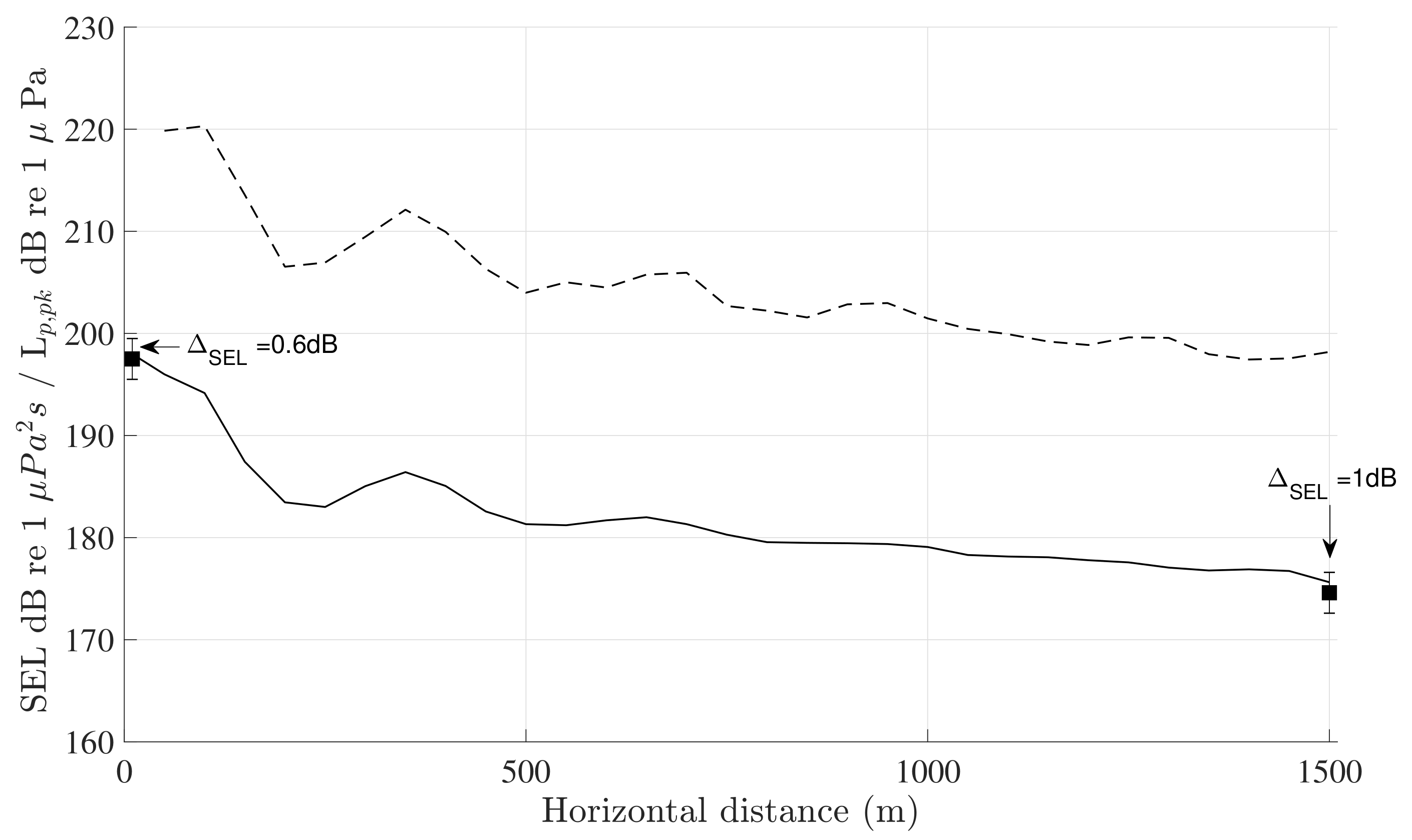
4.1. Evolution of Noise Metrics with Distance

The noise metrics used to assess the radiated underwater sound from percussive pile driving are described in [165] in accordance with the terminology given in [134,166]. Two noise metrics are primarily used: the sound exposure level $L_E$ (or SEL) and the zero-to-peak pressure level ($L_{p,pk}$). The former is given by Equation (2), evaluated now at the specific location of interest, e.g., not depth-averaged, whereas the latter is defined as

$$L_{p,pk}=20{log}_{10}\left(\frac{p_{pk}}{p_0}\right)$$

(31)

In Equation (31), $p_{pk}$ is the zero-to-peak sound pressure that can arise from either a positive or a negative sound pressure, whereas $p_0={10}^{-6}$ Pa in accordance with the work in [134]. Hereafter, the evolution of the SEL and $L_{p,pk}$ with distance in the case of impact piling is discussed for the case study reported by Fricke and Rolfes [120]. The relevant material and geometrical properties are summarised in

Table 2. Input parameters for the simulations at the BARD Offshore I offshore wind farm.

Parameter	Pile	Parameter	Fluid	Upper Soil Layer	Bottom Soil Layer
Length [m]	85	Depth [m]	40	2	∞
Density [kg/m3]	7850	$\rho$ [kg/m3]	1000	1888	1908
Outer diameter [m]	3.35	$c_L$ [m/s]	1500	1705	1725
Wall thickness [mm]	70	$c_T$ [m/s]	-	186	370
Final penetration depth [m]	20	${\alpha }_p$ [ dB/$\lambda$]	-	0.91	0.88
Maximum Blow Energy [kJ]	1370	${\alpha }_s$ [ dB/$\lambda$]	-	1.86	2.77

and the applied hammer force with its frequency spectrum are given in Figure 7. In the case considered, the pile was driven using a MENCK MHU 1900S hydraulic hammer with a ramp energy of about 1370 kJ. The sound levels given by Equations (2) and (31) were also evaluated from the measured pressure time traces at $r=10$ m (mid-water depth) and at $r=1500$ m (2 m above the seabed surface).

Figure 8 shows predictions of the SEL and the $L_{p,pk}$ as a function of the horizontal distance from the pile using the model in [140]. We first note that the model predictions are within the uncertainty of the measuring equipment given the hydrophones’ sensitivity at both locations in which noise measurements were available. Most models described in Section 3.4 are nowadays capable of reproducing measurements with similar accuracy as illustrated in [156,157]. The $L_{p,pk}$ shows larger variation with distance which can be explained by the fact that it is more sensitive to constructive and destructive interference of the acoustic waves in the seawater. In contrast, the SEL, being an integral quantity representing an energy level, shows a much smoother evolution with range, especially at distances larger than 500 m. Please note that these two noise metrics provide no insight as to the frequency content of the radiated sound, i.e., one could possibly retrieve the same levels from two distinct pressure time traces. This is an item worth looking into more carefully in the future [66].

A more in-depth examination of the acoustic field involves the study of the frequency spectrum of the radiated noise. For the case discussed here, the one-third octave band frequency spectra evaluated at a distance of $1.5$ km from the pile are shown in Figure 9 together with the measured one using the values reported in [120] and the model predictions by Tsouvalas et al. [140]. Both models are able to capture the noise spectrum with sufficient accuracy. The frequency bands at which the noise levels are higher depend on the pile diameter and the excitation force characteristics. For typical impact forces of short duration able to excite a wideband acoustic spectrum, the critical frequency bandwidth relates strongy to the pile diameter as will be shown in Section 4.3.

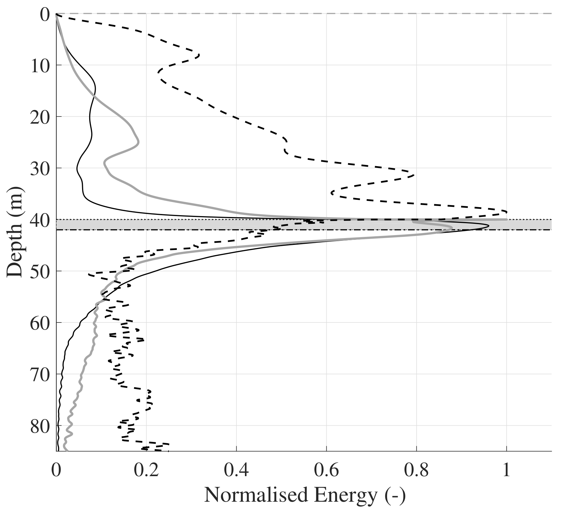
4.2. Energy Flux through the Seawater and the Seabed

Next to the sound levels discussed in Section 4.1, it is instructive to examine the radiated wave field under the prism of the energy flux. An energy flux analysis can be of importance for a number of reasons. First, it contributes to the understanding of the energy transfer through seabed and water together its evolution with increasing distance from the pile. Here, one may think of the direct radiation of noise into the seawater, the secondary noise path through the soil and the energy carried by interface waves travelling along the seabed-water interface. Second, it allows one to explain possible inefficiencies of the noise mitigation strategies as discussed further in Section 5. Third, it gives the possibility to make solid choices on the optimal noise mitigation strategy tailored to the needs of each specific case in terms of the type of mitigation system, the distance from the pile and the deployment strategy.

Figure 10 shows the normalised (to the maximum per location value) energy fluxes calculated by means of the formulae given in [115] at various distances. We note that at close distances to the pile the energy is largely concentrated close to the seabed–water interface due to the presence of high-amplitude Scholte waves. The amplitude of the latter diminish with distance; at 140 m the largest part of the energy is carried by the bulk waves in the water. The compressional waves in the water column experience less attenuation compared to the ones in the seabed and therefore survive at larger distances. In the same lines, one could examine the flux of energy from the seabed to the water to establish the optimum position for the deployment of a noise mitigation system.

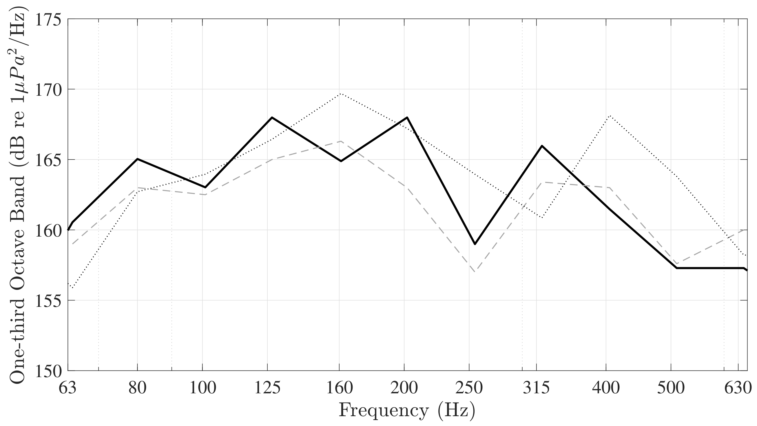
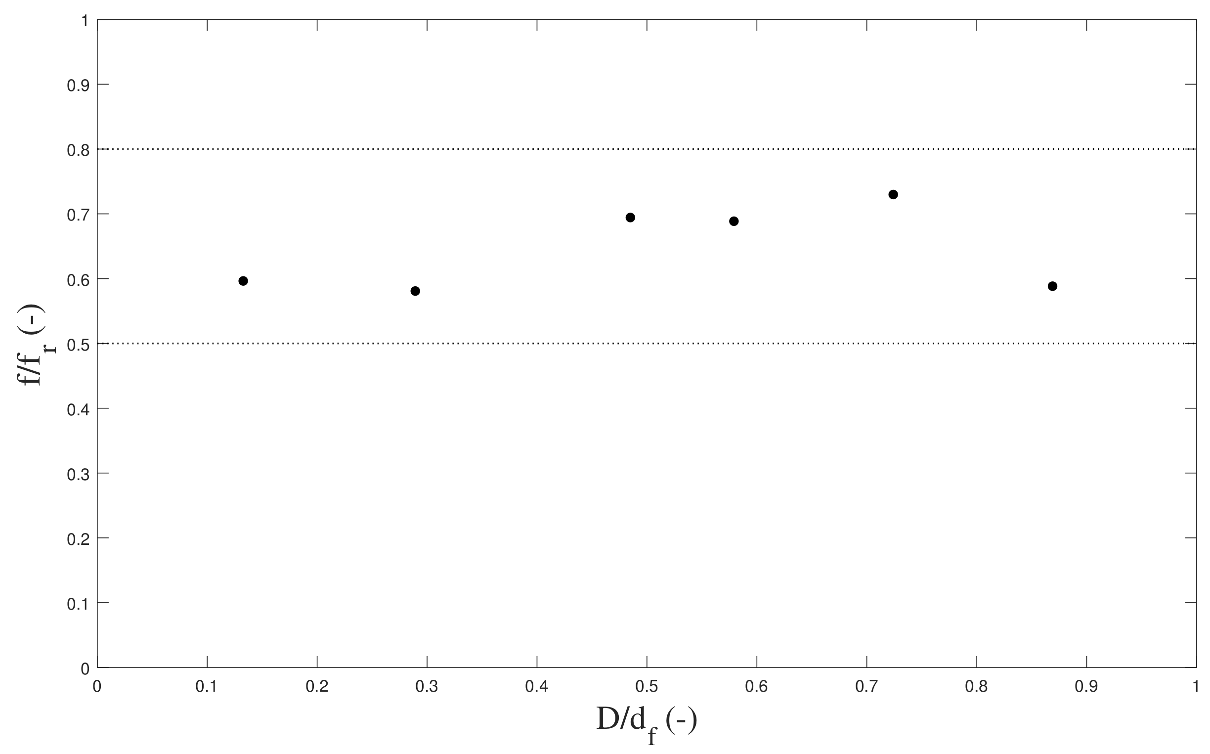
4.3. Noise Spectrum and Pile Size

To analyse the effect of the pile size on the frequency content of the radiated noise, the normalised frequency is introduced, which is defined as the ratio of excitation frequency to the ring frequency of the cylindrical shell $f_r={\left(2\pi R\right)}^{-1}\sqrt{E/\left(\rho (1-{\nu }^2)\right)}$. Model simulations have shown that when $f_{norm}\sim 1.0$, the acoustic radiation pattern shows some peculiar characteristics [19]. In particular, for frequencies between $0.5f_r\le f\le 0.8f_r$, the pressure levels are usually amplified whereas around the ring frequency they drop significantly. This observation actually allows one to a priori estimate the critical frequency range of interest, i.e., the frequency bandwidth at which the majority of the noise is concentrated, based on the knowledge of the pile size alone, as shown in Figure 11.

The geometrical and material characteristics of the cases examined are similar to the ones given in Table 2 but for a new water depth of $d_f=6.9$ m. In Figure 11, the dimensionless frequency ($f/f_r$) in which the maximum pressure occurs is plotted versus the dimensionless diameter of the pile ($D/d_f$) for pile diameters ranging from $0.92$ m $\le D\le 6$ m so that $0.1\le D/d_f\le 0.9$. The pressure amplitudes are normalised with respect to the maximum pressure value at each of the examined cases. This way, the shift of the maximum pressure for the various cases is clearly shown (the pressure value itself is irrelevant in our discussion hereafter). In all cases, the maximum pressure level is reached at $0.5f_r<f<0.8f_r$. In addition, for excitation frequencies close to the ring frequency, a sudden drop in the pressure amplitude is visible in all the examined configurations. At the ring frequency most of the energy introduced by the hammer is absorbed by the shell itself and (almost) no energy radiates into the fluid region. Please note that the above observations hold for symmetric excitations; when non-symmetric modes are excited the radiation pattern may alter significantly [111].

5. Noise Mitigation Strategies

Next to the developments in noise prediction modelling, studies on noise mitigation have also been conducted [167,168,169]. There are in principle two ways to reduce the noise levels caused by pile installation [170]. The first one is the alteration of the noise source mechanism, i.e., the adoption of a different pile driving procedure such that noise emission is reduced at the source. In this respect, one can either modify the force exerted by the impact hammer [171,172] or switch to alternative pile driving methods that avoid the generation of high-amplitude shock waves in the pile, e.g., traditional vibratory piling [16,17], BLUE Piling [173] or Gentle Driving of Piles (GDP) [174].

The second way to reduce the noise is to create a so-called anti-noise barrier around the pile. The noise barriers can be categorised into three primary groups on the basis of the underlying noise reduction principle:

• air bubble curtains in various configurations [175,176,177],
• casings that enclose the pile in the form of either a de-pressurised double-walled cylindrical shell [178] or lightweight inflatable fabrics which build an air-column around the pile and
• resonator-based noise mitigation systems which can take the form of either a fishing net of encapsulated bubbles and foam elements [179,180] or Helmholtz-type resonators [181,182].

Air-bubble curtains achieve noise reduction on the basis of (i) wave reflection upon incidence of the acoustic waves on the air bubble cloud, and (ii) wave attenuation due to the resonating bubbles once the transmitted acoustic waves enter the air bubble cloud. The governing mechanism is primarily determined by the frequency content of the radiated sound (Section 5.1). Pile casings reduce noise due to wave reflection (Section 5.2). Finally, resonator-based systems transform the energy carried by the acoustic waves into vibrations of their own base units, i.e., resonator units act as acoustic energy sinks (Section 5.3). Combinations of the noise reduction principles above are also applied in practice, especially when a single noise mitigation technique proves incapable of reducing the noise levels to within acceptable limits. Please note that the specific techniques discussed in the sequel may be incomplete as new technologies become continuously available [183].

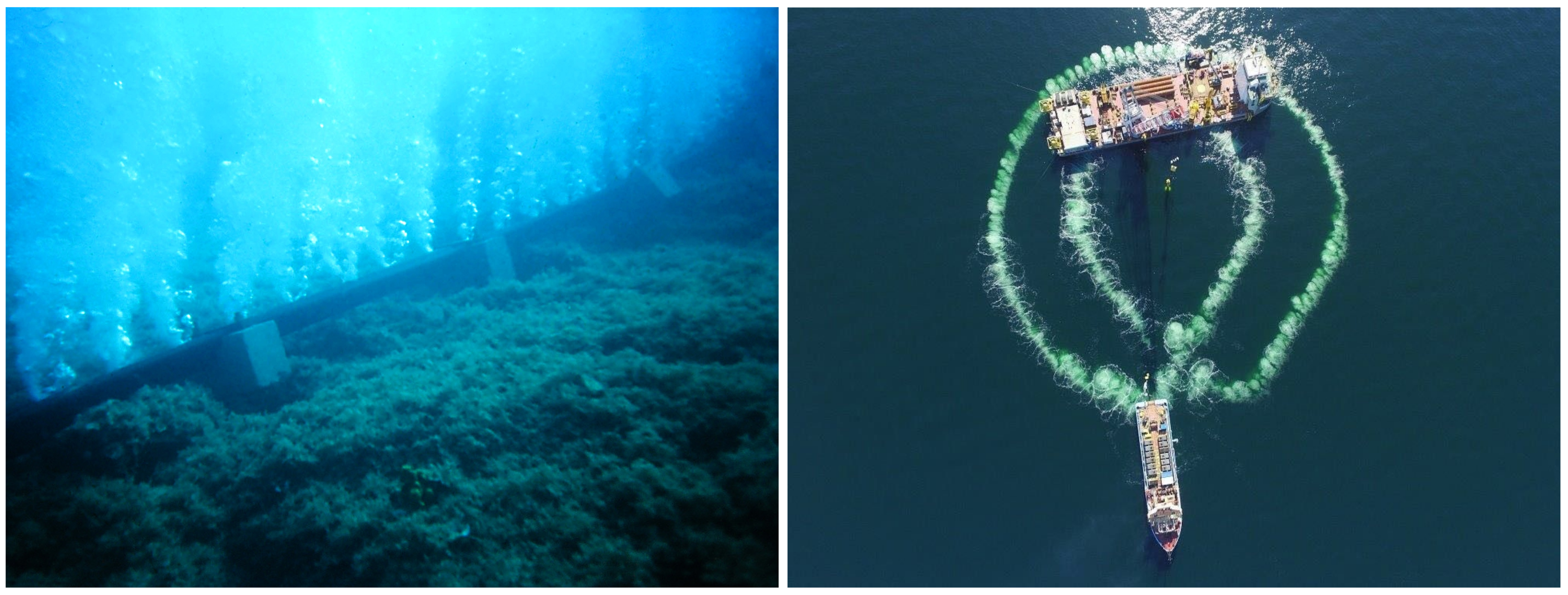
5.1. Air Bubble Curtains

The most widely adopted method to mitigate underwater noise is the development of a noise barrier in the seawater column that consists of rising air bubbles. The air bubble cloud is placed around the pile at a given distance in the form of a bubble curtain [175], which is formed by freely rising bubbles created by compressed air injected through series of perforated pipes positioned on the seabed surface (Figure 12). The compressed air is supplied by an air compressor usually positioned on the installation vessel.

The impedance contrast between the seawater and the air bubble curtain is significant due to the large differences in density and compressibility of the two media. Although the volume of the supplied air is usually only a small fraction in the mixture, the change in the compressibility of the air–water medium is rather significant [184]. It was originally thought that the resonance of the air bubbles is key to an effective noise reduction. However, experiments have shown that the formation of a dense layer of slow-rising bubbles of small radii provides an improved noise reduction when compared to the same air–volume supply distributed in fewer large-size air bubbles [177,185]. For piles with diameters larger than 6 m, that are used as foundation piles of offshore wind turbines, the acoustic energy is radiated at frequencies between 100 and 400 Hz (Section 4.3). At such low frequencies, the desired bubble radii to stimulate resonance range between 8 mm and 32 mm near the surface and between 14 mm and 50 mm at a water depth of 30 m. The creation of bubbles of such large radii is rather difficult, especially in the harsh offshore environment. Thus, despite the role that resonance phenomena may play in sound absorption, the wave reflection caused by the impedance mismatch between the seawater and the air bubble curtain seems to be the single most significant mechanism leading to noise reduction.

To clarify the behaviour of an air bubble cloud of certain configuration using the effective medium theory approach [186,187], one can study Figure 13 in which the effect on the wave speed and attenuation of the air bubble cloud is illustrated for varying bubble radii. Considering the frequency range associated with the installation of large foundation piles ($f<600$ Hz) and the bubble radii adopted usually in practice ($\alpha \le 5$ mm), it can be seen that the air-volume fraction plays the crucial role in the estimation of the wave speed in the medium for frequencies $f<0.7f_r$. As for bubbles of small radii the resonance frequency is relatively high, the wave speed in the bubbly medium can be considered quasi-constant in most practical applications [188]. Only around the resonance frequency of the air bubbles, the dispersive characteristics of the bubbly medium may become critical; however, these frequencies remain largely outside the frequency range of interest in most practical applications dealing with the installation of large foundation piles in offshore wind.

Air bubble curtains are distinguished into two main groups: the Little Bubble Curtain (LBC) and the Big Bubble Curtain (BBC). This distinction reflects mainly the horizontal distance from the pile at which the bubble curtain is positioned; the LBC is placed at the vicinity of the pile, whereas the BBC is positioned at large distances. Several variations of the LBC have been tested, namely, layering ring systems, bubble curtains confined by steel, fabric or plastic casings [189] and vertical arrangement of perforated tubes around the pile [190]. The confinement of the rising bubbles, whenever possible, serves to avoid the drift of the air bubbles due to the tidal currents. The noise reduction varies among the various systems and depends on the successful encirclement of the pile which is of utmost importance for noise mitigation. Measurements with the use of the LBC have shown an attenuation in the range of 10 to 15 dB in the $L_E$ [176]. The noise reduction was negligible at frequencies below 50 Hz and was the highest at the frequency bandwidth 1–10 kHz. Although the LBC gained some popularity at the early stages of development, such systems have been applied only in a few commercial projects.

In contrast, Big Bubble Curtains (BBC) have been tested extensively with the number of commercial projects in which BBC variants have been applied exceeding 1000 up to 2018 [183]. In Figure 12, the installation of a double BBC (DBBC) is shown at the offshore wind farm (OWF) Wikinger. The noise attenuation of the BBC is believed to be superior to that of the LBC mainly because of the potential of the former to mitigate, additionally, the energy that leaks from the soil back to the seawater. Next to the applications in impact pile driving, the potential of air bubble curtains to reduce impulsive sound has also been explored in the area of underwater airgun stimuli [191,192].

5.1.1. Modelling the Air Bubble Curtain

There have been several attempts to include air bubble curtains in noise prediction models [188,193,194,195]. In principle, the modelling of the air bubble curtain is based on the effective medium theory approach [184,186,187] yielding a column of air-water mixture of certain thickness of significantly different compressibility compared to the surrounding seawater. Results are discussed hereafter for the model developed by Tsouvalas and Metrikine [188], which consists of the pile, the surrounding water and soil media and the air bubble curtain as shown in Figure 14. In this model, the air bubble curtain is assumed of equal thickness and composition throughout the whole water depth. In a more recent model by Bohne et al. [195], this assumption is somewhat relaxed and more realistic distributions of the air bubble cloud are considered. The division of the exterior to the pile domain into three regions allows for a straightforward mode-matching solution in the same lines as described in Section 3.3.1, which is omitted here for the sake of brevity.

Numerical simulations using the model in [188,196] have confirmed experimental observations:

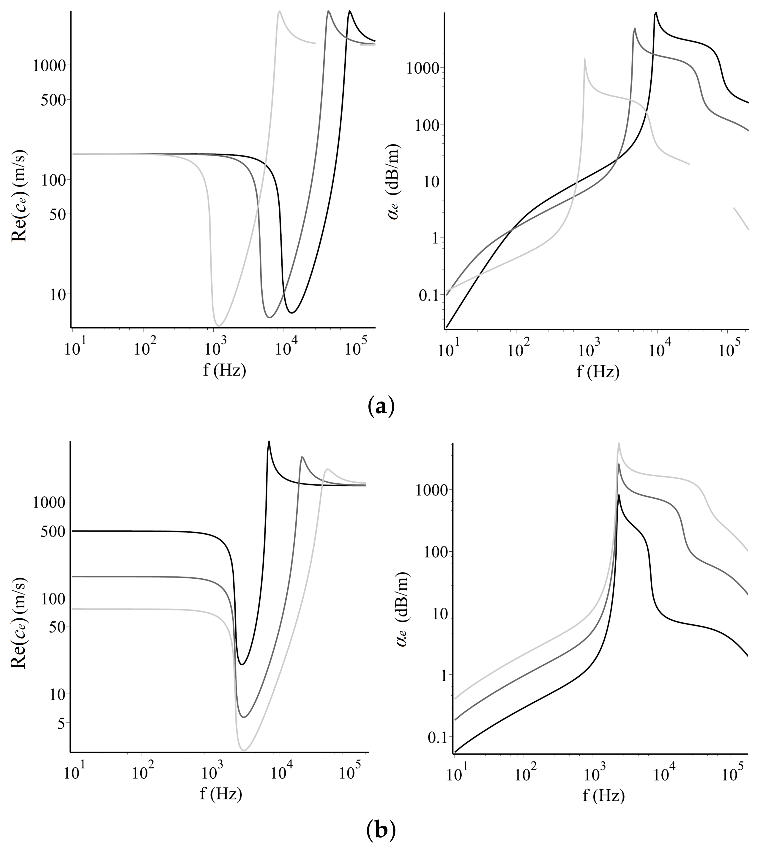
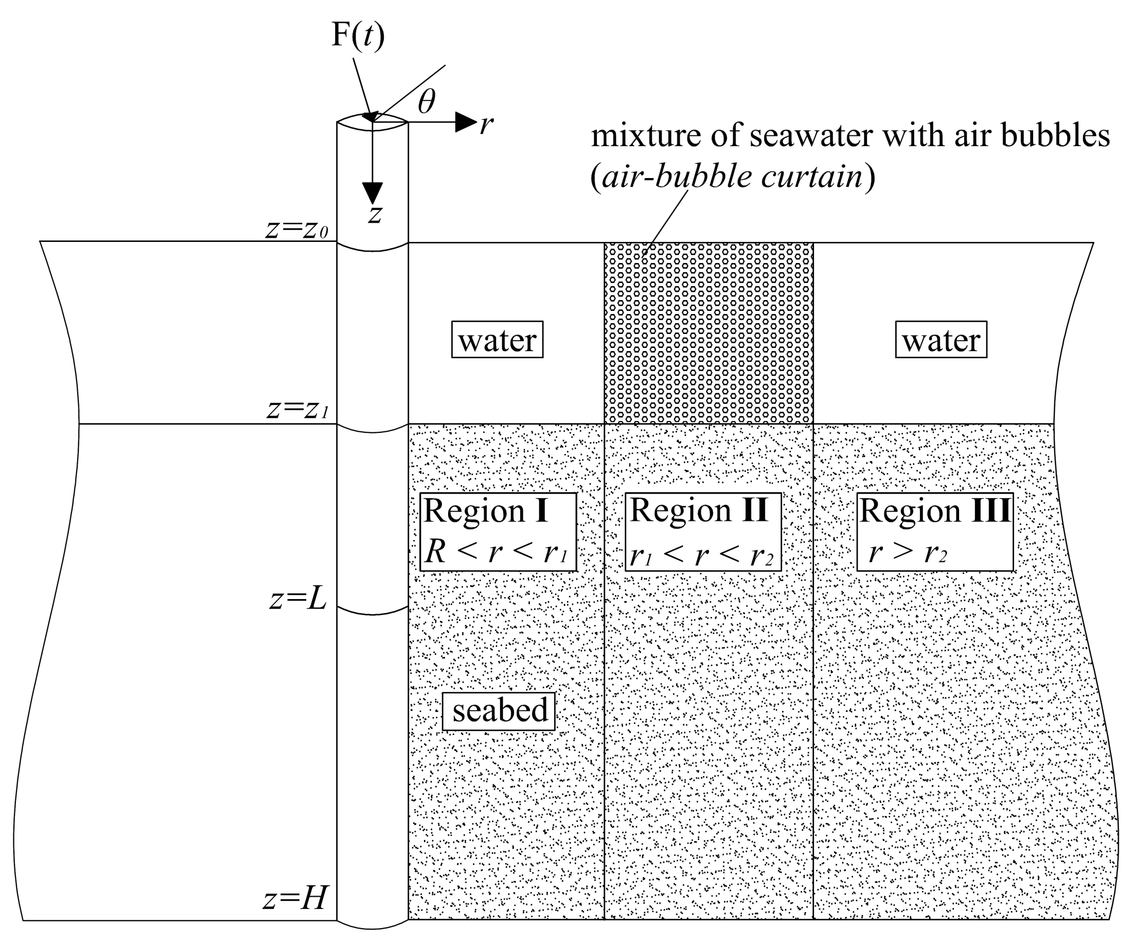
• The primary mechanism of noise reduction in the low-frequency range is the impedance mismatch between regions I and II (Figure 13). The attenuation of the waves in the bubbly layer seems not to be the governing factor in the noise reduction, mainly because of the relatively high resonance frequency of the small bubbles usually applied in practice (Figure 13).
• The effectiveness of the air bubble curtain is higher for an increased air–volume fraction in the bubbly medium (Figure 13). This has also been reported in [185]. An increase of the air–volume fraction results at a decreased wave velocity. This, in turn, yields a higher impedance contrast between the seawater and the bubbly medium (regions I and II).
• An increase in the thickness of the curtain does not lead to an increased noise reduction at the frequency range of interest in most cases. This holds for bubbly mixtures in which the principal mechanism of noise reduction is the impedance mismatch between the seawater and the air bubble curtain as explained earlier.
• The distance at which the bubble curtain is placed can influence its effectiveness. An increase in the horizontal distance leads to an increased noise reduction when all other parameters remain the same. This has been confirmed more recently by the cases analysed in [195], in which a more detailed explanation is given. This observation also explain why the noise reduction achieved by the BBC is superior to that of a LBC.

5.2. Pile Casings

Casings are systems that are placed around the pile and enclose the latter entirely along the seawater column. The principle of sound attenuation is wave reflection so that the emitted sound waves are trapped in the volume between the pile and the casing. There are several variants of this type available to date: noise mitigation screens and lightweight inflatable fabrics that allow the generation of an air column between the pile and the exterior seawater domain.

5.2.1. Noise Mitigation Screens

The Noise Mitigation Screen (NMS) (IHC Iqip) consists of a double-walled cylindrical shell made of steel that is placed around the pile at a distance of a few meters from the pile surface (see Figure 15). The gap between the inner and the outer wall of the NMS is filled with air. The system can be combined with an air bubble curtain that fills the inter-space between the pile and the inner wall of the NMS yielding a combined LBC-NMS system [178]. Subsequent phases of the installation of a monopile with the NMS at the German offshore wind farm Riffgat are shown in Figure 15. Please note that the system depicted in Figure 15 is an old version and newer versions are available [183].

The principle mechanism of noise mitigation is the creation of a shielding effect around the pile. The sound waves that irradiate by the surface of the pile are incident upon the inner wall of the NMS. As a consequence, most of the energy reflects backwards into the closed region formed by the pile and the inner wall of the NMS. Another part of the energy sets the inner wall into motion which in turn radiates sound into the inter-space between the two walls of the NMS. The relatively low density of the air cannot set the outer wall into motion which in fact results in an efficient acoustic decoupling of the two walls. Thus, the largest part of the energy irradiated in the form of pressure waves in the seawater is either trapped in the region between the pile and the inner wall of the NMS or dissipated in the double-walled NMS by several mechanisms. The NMS has been used in excess of 400 commercial projects until mid 2018 and the noise reduction achieved in terms of the SEL is in the order of 12∼17 dB with the upper limit holding when it is applied simultaneously with the BBC.

5.2.2. Lightweight Inflatable Fabrics

The HydroNAS (HydroNAS) uses a lightweight inflatable fabric, which is restrained internally, to build a continuous column of air surrounding the pile from the seabed to the surface. Upon the inflation of the fabric, a fixed volume panel of air is created which maintains a specified geometry underwater. The cells are modular, stackable and can be configured to fit any water depth and pile size. The system is at its early stage of development and has not yet been tested in full-scale offshore environments.

5.3. Resonator-Type Systems

Resonators consist of an array of resonating units that are deployed around the pile to absorb the emitted sound. Unlike the previous methods which are based on wave reflection, resonator-type systems work as acoustic energy sinks, i.e., the acoustic energy emitted is absorbed by the resonator devices causing internal (mechanical) vibrations of the latter [181]. There are several options to design such a device. In the sequel, two types are discussed that have been already tested full-scale in offshore environments.

5.3.1. Hydro-Sound-Dampers (HSD)

HSD use nets of air-filled balloons and special PE-foam elements with high dissipative characteristics to reduce noise levels caused by impact piling. A typical installation set-up with the use of HSD is shown in Figure 16 Left. HSD rely on multiple mechanisms to reduce the underwater noise:

• resonant effects of the air-filled balloons and the PE-foam elements fixed in the fishing net. The HSD-elements are adjustable both in terms of diameter and positioning on the net. Thus, they can be tuned in order to achieve optimum noise reduction at frequencies associated with the energy of acoustic waves of specific wavelengths;
• dissipation and material damping effects according to the chosen materials and the injected pressure in the air balloons; and
• reflection of the sound waves at the interface between the water and the fishing net caused by the impedance mismatch (although this mechanism is less efficient in this case compared to the case of a dense air bubble curtain).

The efficacy of the HSD in reducing the noise levels depends on the frequency and volume ratio of the HSD-elements in the net with ratios of about 1–2% to be sufficient to obtain acceptable noise reduction [197]. The system has been used in more than 250 commercial projects until 2018.

5.3.2. Helmholtz Resonators (AdBm-NAS)

The AdBm-NAS consists of standard size panels with submersible air-filled Helmholtz resonators that encircle the pile during construction. To accommodate the particular needs of a specific project, the supplier offers the resonator panels either with a frame or on their own. In the latter case, the steel framework holding the system needs to be designed and fabricated by another contractor. The AdBm system completed successfully a full-scale demonstration test in 2018 [182] and is expected to be used in commercial projects in the near future.

5.4. Overview of Mitigation Techniques and Spectral Insertion Loss

In

Table 3. Overview of the most widely used noise mitigation systems, their principal mechanism of noise attenuation, and their broadband noise reduction levels. Installed pile data reflect experience gathered until mid 2018.

Mitigation System	Principal Mechanism of Noise Reduction	Number of Piles	ΔSEL
Big Bubble Curtain	Impedance mismatch between the water and the bubbly medium. Noise reduction depends upon the supplied air–volume, size of the air bubbles, successful encirclement of the radiating source and thickness of the bubble screen, single or double BBC.	>1000	∼13 for the single BBC and ∼17 for the double BBC
Noise Mitigation Screen	Shielding effect around the pile, reflection and absorption of the energy. Noise reduction depends upon the space between the inner and the outer wall, the distance between the pile and the inner screen, the isolation of the outer wall from the ground vibrations, the additional presence of a BBC around the screen.	>400	∼12 without the BBC and ∼17 with the BBC
Hydro-Sound Dampers	Scattering and absorption of the energy from the resonating bubbles and reflection of sound at the HSD-net/water interface. Noise reduction depends upon the number, the size and the configuration of the air balloons and PE-foam elements of the system. The system can be tuned to absorb acoustic energy at certain frequency bandwidths.	>250	∼15

, an overview of the most widely used noise mitigation systems is given together with the number of commercial projects in which they have been applied until 2018. In addition, an indication of their broadband noise reduction in terms of the Sound Exposure Level (ΔSEL) is included for comparison. It is important to note that only when the various systems are tested under the same installation settings, i.e., water depth, soil properties, pile dimensions and input energy, is there solid ground for a direct comparison of their mitigation efficiency.

Next to the above, it is important to note that apart from the case of the air bubble curtain which was discussed in Section 5.1.1, scientific publications reporting modelling of other noise mitigation systems are rather scarce. This can be explained by the fact that the complexity of these systems requires an in-depth numerical investigation which can be achieved only by means of detailed FE models. However, with the increasing use of such systems, the modelling of noise mitigation will become essential in the future.

In Figure 17, an overview of the noise reduction (spectral loss) of the various systems is given in one-third octave bands as reported by Bellmann [185]. The noise reduction presented here is only indicative and the efficiency of the various systems in reducing the noise levels can vary significantly upon different soil conditions and water depths. Keeping that in mind, the noise reduction spectra given in Figure 17 provide only a rough indication of the spectral loss when a given mitigation system is applied under similar, to the tested case, conditions. By examining Figure 17 under this prism, one may observe the following.

• No technique can reduce the noise levels effectively below 20 Hz.
• The noise reduction of all techniques is optimum at frequencies above 200 Hz.
• Only the double BBC and the NMS together with the BBC are capable of reducing the noise levels by more than 20 dB at frequencies ranging from 125 Hz up to 8 kHz. In the other techniques, the noise reduction is usually less and outside the frequency range of interest (>500 Hz).
• The spectral insertion loss depends strongly on the particular location as can be concluded by the application of the same system (BBC) in different projects.

6. Future Challenges

The state-of-the-art in predictive modelling of sound due to impact piling includes a detailed description of the pile interacting (linearly) with soil and water. Other elements, such as the anvil positioned at the pile head and the hydraulic hammer, are usually disregarded in the acoustic models and are substituted by a force applied at the top of the pile. Such a force can be estimated on the basis of a so-called driveability model with the focus being placed on the nonlinear pile–soil interaction including the details of the hammer–anvil system [120]. These models have been proven capable of reproducing measurements with satisfactory accuracy in terms of the SEL and the $L_{p,pk}$ in the case of impact piling [46,151,156,157]. Publications reporting a more complete validation in terms of physical quantities as obtained by actual measurements, such as the frequency spectra and the time traces, are rare with only a few exemptions [19,107,120]. Having dealt with the basic configuration described earlier in Section 3, the focus is gradually shifted towards the following research topics.

• Advanced modelling of the seabed, either by introducing a modified elastic continuum description with frequency-dependent wave speed and attenuation [198,199,200] or by adopting the theory of poro-elasticity by Biot [201,202,203,204].
• Probabilistic modelling in which the uncertainties in the characterisation of the geometry or the properties of the acousto-elastic region are propagated at larger distances from the pile [155];
• Pile driving noise predictions in range- and/or angular-dependent environments.
• Non-symmetric hammer force [107,111], or inclined piles [205,206] yielding an azimuthally dependent acoustic field.
• Simultaneous pile progression into the soil with noise prediction in the near-field (nonlinear pile-soil interaction).
• Challenges associated with the modelling of the various noise mitigation systems and demonstration of the efficacy of those systems for piles of larger diameters (8 m) and deeper waters (>45 m).

These items are discussed in more detail below.

6.1. Advanced Modelling of the Seabed

The marine sediment is traditionally described as an acoustic medium, with some extra attenuation to accommodate energy loss in different waveforms, for the modelling of underwater acoustics generated by pile driving [83,101,207]. More advanced methods for the description of marine sediments do exist and can be divided into three main groups: The first group treats the seabed as a classical elastic continuum with a high Poisson’s ratio (close to 0.5) to account for the increased ratio of P- to S-wave speeds [46]. Typically, P-wave speeds take values close to, or higher than, 1500 m s⁻¹ which reflects the speed of sound waves in the water, while S-wave speeds can be lower than 100 m s⁻¹ for the upper few meters of the seabed [208]. The second group includes the so-called grain-shearing (G-S) models, indented to represent wave propagation in unconsolidated granular media, in which the mineral grains are in contact but unbonded [198,199,200]. This group introduces a frequency dependence in the material properties (phase speeds and attenuation of the waveforms) but is otherwise similar to the classical elastic description above. Models which adopt a solution to the vibroacoustic problem in the frequency domain can typically accommodate such frequency-dependent properties in a straightforward manner [142]. The third group treats the continuum as a poroelastic medium and is based on the well-established theory of Biot [201,202].

Leaving the acoustic models aside, it seems that an elastic description of the seabed with frequency dependent constants [198,199,200], is a fair compromise between the classical elastic description and the complete dynamic poroelasticity theory of Biot [201], Biot [202]. First, such a description allows the (indirect) capturing of the energy loss in the slow P-wave form without explicitly introducing an extra degree of freedom in the model (no extra computational demand). When compared to the Biot model it only neglects the slow compressional mode, as the dispersive characteristics of the other waveforms can be accounted for indirectly [200]. Second, it is based on the knowledge of only a few material parameters which can be retrieved on the basis of standard in situ geotechnical investigation. On the contrary, Biot’s model would require the knowledge of a large number of parameters [209], which are generally unknown from the standard geotechnical investigation that is usually conducted on site prior to the installation of piles.

Given the discussion above, one may conclude that there is limited added value in complicating the noise prediction models with a full poro-elastic description of the seabed, especially when the adoption of frequency-dependent properties in the elastic model is incorporated [46,140]. One may argue that there can be an added value in considering the full poro-elastic description of the seabed for the pile-soil interaction in the vicinity of the pile in order to accurately capture the sound generation mechanism. However, one should not overlook that the nonlinear pile–soil interaction involves many more uncertanties, including the complex frictional dynamics at the soil–pile interface; thus, an attempt to complicate the seabed description alone seems not justified. To the best of the author’s knowledge, no model dedicated to pile driving acoustics to date incorporates the full poro-elastic description. The extra effort in developing such a detailed model should, however, be balanced against some practical considerations, such as the difficulty to collect the input parameters, the lower computational efficiency and the many other uncertainties in the prediction of the sound field.

Next to the seabed modelling, the consideration of more advanced description of the sea surface is a point of attention especially when it comes to propagation of the sound waves at large distances. If one considers only the far-range modelling several option exists [210,211,212].

6.2. Quantification and Propagation of Uncertainties

Most studies on pile driving acoustics report deterministic analyses, i.e., a few scenarios are selected and the sound field is predicted with the aim to capture the possible uncertainty in a few parameters. Such a modelling approach is by far not systematic in spotting the key parameters contributing to uncertainty nor can it be used in a generic framework of uncertainty quantification. Given the large uncertainty in many modelling parameters, especially when it comes to the pile–soil (nonlinear) interaction and the characterisation of the seabed, a probabilistic approach that would accommodate a large number of (fast) simulations is largely missing.

A first attempt to follow a probabilistic framework in noise prediction by impact piling is reported by Lippert and von Estorff [155]. However, in that study, the seabed was described by an acoustic model and a (computationally heavy) Monte Carlo approach was chosen for capturing the uncertainty in the seabed properties. A possible explanation for the relatively marginal contributions in this respect can be attributed to the fact that (most) noise prediction models in impact piling are computationally demanding and thus not suited for a large number of probabilistic simulations. On the one hand, the necessity to re-iterate back to the source model that includes the full pile–soil–fluid configuration every time a model parameter changes is computationally demanding. On the other hand, the idea to separate the near-source model used to identify the source from this iterative procedure and to focus on the wave propagation alone is largely prohibitive since every time a parameter changes the source mechanism alters. To overcome these limitations, the semi-analytical models described earlier in Section 3.3 [107,108,109,110,111,112] may offer an attractive alternative since they have a competitive advantage in terms of computational speed. Next to the semi-analytical formulations above which aim at capturing most of the important characteristics of the pile driving process with minimum computational effort, the development of cheap surrogate or reduced-order models is common practice. For acoustic systems, the construction of a reasonably accurate surrogate model can become a challenging task [213].

Next to the model requirements, the adoption of more advanced mathematical tools to accommodate the propagation of uncertainty systematically is vital in increasing the speed of such probabilistic computations. Monte Carlo simulations are computationally heavy especially when the number of parameters to vary is large. More advanced mathematical tools that have been applied successfully in other research areas can be of added value here [214,215,216,217].

6.3. Three-Dimensional Domains and Non-Symmetric Responses

Almost all models to date adopt a cylindrically symmetric configuration both in terms of the loading scheme (hammer force applied at the pile head) and the geometry of the acousto-elastic domain in the near-field. In the far-field sound propagation, classical acoustic approaches can deal with varying bathymetry and three-dimensional effects based on either energy flux based methods [101,161,162], the adoption of the parabolic equation (PE) [83,96,103] or hybrid approaches based on Weston’s flux [218] and normal mode theories [219].

Regarding the propagation of sound from pile driving in angular- and depth-dependent environments, a recent paper by von Pein et al. [158] worth mentioning. Again, the near-field model assumes an axisymmetric configuration and is modelled in a FEM; however, three-dimensional effects are accounted for at ranges larger than 1km by means of the parabolic equation (PE) method. The study on the effect of varying bathymetry is thoroughly looked upon. It is expected that such studies will gain momentum in the future, especially, if offshore wind farms are constructed in areas in which bathymetric variations are strong.

A few models incorporate non-symmetric forces at the pile head [107,111]. In the work by Deng et al. [111], it is shown that the excitation of higher modes of vibration of the shell structure (in terms of the circumferential wavenumber) may be of some significance for the noise field generated. However, this study does not report any validation with measurement data. In the monograph by Tsouvalas [19], a comparison with measured shell responses shows that higher circumferential modes are excited by the hammer impact, which can be attributed to small inclination in the pile or non-vertical positioning of the hammer. The excitation of higher vibration modes and the effect on the acoustic field is an item worth looking upon in the near future. A proposed mathematical solution to accomondate this effect in a model that includes an elastic description of the seabed is presented in [115] and in more detailed manner in [19]. However, this solution technique has not yet been fully implemented. A recent study by Amaral et al. [206] shows that inclined piles generate an acoustic field with a strong azimulthal depedence with variations in the (measured) radiated sound field along opposing azimuths of up to 10 dB or more. Similar differences may be expected also in the case in which a non-vertical force is applied at the pile head but such studies are not yet available.

6.4. Pile Progression and Simultaneous Noise Prediction

The nonlinear frictional dynamics that take place at the pile-soil interface are complex and not well understood. Some work in this respect trying to identify the frictional losses at the pile–soil interface during piling has been carried out by Fritsch [220]. To date, all existing vibroacoustic models overlook these nonlinear effects and assume that full contact between the pile and the soil is preserved at all times. A few models do consider frictional losses locally at the pile–soil interface [99,100,107,111,154] but not the true nonlinear pile-slip dynamics. Thus, all existing models silently hypothesise that by excluding the pile slip in the prediction of noise the error is marginal. Likely, in the case of impact piling, noise measurements seem to confirm the validity of this hypothesis [120].

In contrast, one should be cautious in generalising this observation to other forms of pile installation in which the progression of the pile into the soil is more smooth. A possible case in which pile progression may be key to accurately capture noise prediction is when vibratory devices are used to install the foundations piles. In contrast to impact piling, which generates a shock wave travelling down the pile inducing local slip at the position of the wave front, in vibropiling standing waves are generated and the pile is gradually pushed into the soil. Thus, the mechanism of pile driving is considerably different as well as the sound field generated [45,133].

It is expected that noise predictions with models calibrated for impact piling will largely fail to reproduce measured data when alternative methods are used to drive the piles. In other words, a mere substitution of the impact force by another one mimicking the vibratory device may be not sufficient to provide a reliable prediction of the sound field. The energy lost into overcoming the frictional resistance of the pile shaft may be key in the latter case together with the continuous change in the penetration depth of the pile into the seabed. This hypothesis still remains to be verified.

6.5. Modelling the Noise Mitigation

A lot of effort has been placed in the modelling of the sound generation in the free-field, i.e., in the absence of any noise mitigation applied. Such predictions are very important to understand the noise emission paths and to design appropriate noise mitigation systems. However, the research on the modelling of the various noise mitigation systems is rather limited. From all the mitigation systems described in Section 5, most modelling efforts have been focused on air bubble curtains alone [188,193,194,195].

With the increase in the size of the foundation piles used in offshore wind, the energy spectrum of the radiated noise will shift towards lower frequencies. Subsequently, the use of alternative methods of noise mitigation that can be tuned effectively to absorb the acoustic energy at the very low frequencies will gain popularity. In addition, there will be a need for models that systematically provide reliable noise predictions when specific noise mitigation systems are applied. This will eventually also help to optimise the deployment of such systems. To the best of the author’s knowledge validated models which include the various noise mitigation systems are largely missing.

7. Concluding Remarks

Models to predict the underwater noise in the case of impact piling, and without the inclusion of noise mitigation, have reached a mature state of development. On the basis of the preceding discussions, the following open challenges are identified.

• Development of acoustic models suitable for vibro-piling and other installation technologies. Nowadays, all models focus on impact piling since this method is primarily used offshore and generates significant noise pollution. However, in order to reduce the costs, the offshore market will shift towards more silent methods of pile installation. Consequently, the need will arise to provide tools for noise assessment also in those cases.
• Modelling of the various noise mitigation systems to systematically study and optimise their deployment.
• Quantification and propagation of uncertainties in a systematic and computationally efficient manner to allow for sound judgements of the noise levels to be expected in different environments.
• Incorporation of three-dimensional domains and non-symmetric force excitations.
• Integration of the predictions by vibroacoustic models to the work accomplished by the marine biologists to provide unified tools for environmental impact assessment (EIA) studies.

References

1. Breton, S.P.; Moe, G. Status, plans and technologies for offshore wind turbines in Europe and North America. Renew. Energy 2009, 34, 646–654. [Google Scholar] [CrossRef]
2. Sun, X.; Huang, D.; Wu, G. The current state of offshore wind energy technology development. Energy 2012, 41, 298–312. [Google Scholar] [CrossRef]
3. Athanasia, A.; Anne-Bénédicte, G.; Jacopo, M. The offshore wind market deployment: Forecasts for 2020, 2030 and impacts on the European supply chain development. Energy Procedia 2012, 24, 2–10. [Google Scholar] [CrossRef] [Green Version]
4. Kaldellis, J.; Kapsali, M. Shifting towards offshore wind energy—Recent activity and future development. Energy Policy 2013, 53, 136–148. [Google Scholar] [CrossRef]
5. Perveen, R.; Kishor, N.; Mohanty, S.R. Off-shore wind farm development: Present status and challenges. Renew. Sustain. Energy Rev. 2014, 29, 780–792. [Google Scholar] [CrossRef]
6. Fried, L.; Shukla, S.; Sawyer, S. Chapter 26—Growth Trends and the Future of Wind Energy. In Wind Energy Engineering; Letcher, T.M., Ed.; Academic Press: Cambridge, MA, USA, 2017; pp. 559–586. [Google Scholar] [CrossRef]
7. Bilgili, M.; Yasar, A.; Simsek, E. Offshore wind power development in Europe and its comparison with onshore counterpart. Renew. Sustain. Energy Rev. 2011, 15, 905–915. [Google Scholar] [CrossRef]
8. Byrne, B.W.; Houlsby, G.T. Foundations for Offshore Wind Turbines. Philos. Trans. Math. Phys. Eng. Sci. 2003, 361, 2909–2930. [Google Scholar] [CrossRef]
9. Oh, K.Y.; Nam, W.; Ryu, M.S.; Kim, J.Y.; Epureanu, B.I. A review of foundations of offshore wind energy convertors: Current status and future perspectives. Renew. Sustain. Energy Rev. 2018, 88, 16–36. [Google Scholar] [CrossRef]
10. Wu, X.; Hu, Y.; Li, Y.; Yang, J.; Duan, L.; Wang, T.; Adcock, T.; Jiang, Z.; Gao, Z.; Lin, Z.; et al. Foundations of offshore wind turbines: A review. Renew. Sustain. Energy Rev. 2019, 104, 379–393. [Google Scholar] [CrossRef] [Green Version]
11. Lozano-Minguez, E.; Kolios, A.; Brennan, F. Multi-criteria assessment of offshore wind turbine support structures. Renew. Energy 2011, 36, 2831–2837. [Google Scholar] [CrossRef] [Green Version]
12. O’Kelly, B.; Arshad, M. 20—Offshore wind turbine foundations–analysis and design. In Offshore Wind Farms; Ng, C., Ran, L., Eds.; Woodhead Publishing: Cambridge, UK, 2016; pp. 589–610. [Google Scholar] [CrossRef]
13. Negro, V.; López-Gutiérrez, J.S.; Esteban, M.D.; Alberdi, P.; Imaz, M.; Serraclara, J.M. Monopiles in offshore wind: Preliminary estimate of main dimensions. Ocean Eng. 2017, 133, 253–261. [Google Scholar] [CrossRef]
14. European Wind Energy Association (EWEA). Offshore Wind in Europe—Key Trends and Statistics 2018; Technical Report; WindEurope asbl/vzw: Brussels, Belgium, 2019. [Google Scholar]
15. Thomsen, K.E. Chapter Eleven—Commonly Used Installation Methods. In Offshore Wind; Thomsen, K.E., Ed.; Elsevier: Boston, MA, USA, 2012; pp. 157–184. [Google Scholar] [CrossRef]
16. Jonker, G. Vibratory Pile Driving Hammers for Pile Installations and Soil Improvement Projects. In Proceedings of the Offshore Technology Conference, Houston, TX, USA, 27–30 April 1987. [Google Scholar] [CrossRef]
17. Warrington, D. Theory and Development of Vibratory Pile-Driving Equipment. In Proceedings of the Offshore Technology Conference, Houston, TX, USA, 1–4 May 1989. [Google Scholar] [CrossRef]
18. Viking, K. Vibro-Driveability—A Field Study of Vibratory Driven Sheet Piles in Non-Cohesive Soils. Ph.D. Thesis, KTH Byggvetenskap, Stockholm, Sweden, 2002. [Google Scholar]
19. Tsouvalas, A. Underwater Noise Generated by Offshore Pile Driving. Ph.D. Thesis, Delft University of Technology, Delft, The Netherlands, 2015. [Google Scholar] [CrossRef]
20. Farcas, A.; Thompson, P.M.; Merchant, N.D. Underwater noise modelling for environmental impact assessment. Environ. Impact Assess. Rev. 2016, 57, 114–122. [Google Scholar] [CrossRef] [Green Version]
21. Popper, A.; Hastings, M. The effects of anthropogenic sources of sound on fishes. J. Fish Biol. 2009, 75, 455–489. [Google Scholar] [CrossRef] [PubMed]
22. Slabbekoorn, H.; Bouton, N.; van Opzeeland, I.; Coers, A.; ten Cate, C.; Popper, A.N. A noisy spring: The impact of globally rising underwater sound levels on fish. Trends Ecol. Evol. 2010, 25, 419–427. [Google Scholar] [CrossRef] [Green Version]
23. Finneran, J.J. Noise-induced hearing loss in marine mammals: A review of temporary threshold shift studies from 1996 to 2015. J. Acoust. Soc. Am. 2015, 138, 1702–1726. [Google Scholar] [CrossRef]
24. Erbe, C.; Dunlop, R.; Dolman, S. Effects of anthropogenic noise on animals. In Effects of Anthropogenic Noise on Animals; Springer: New York, NY, USA, 2018; pp. 277–309. [Google Scholar] [CrossRef]
25. Bailey, H.; Senior, B.; Simmons, D.; Rusin, J.; Picken, G.; Thompson, P.M. Assessing underwater noise levels during pile-driving at an offshore windfarm and its potential effects on marine mammals. Mar. Pollution Bull. 2010, 60, 888–897. [Google Scholar] [CrossRef]
26. Brandt, M.; Diederichs, A.; Betke, K.; Nehls, G. Responses of harbour porpoises to pile driving at the Horns Rev II offshore wind farm in the Danish North Sea. Mar. Ecol. Prog. Ser. 2011, 421, 205–216. [Google Scholar] [CrossRef] [Green Version]
27. Tougaard, J.; Kyhn, L.A.; Amundin, M.; Wennerberg, D.; Bordin, C. Behavioral reactions of harbor porpoise to pile-driving noise. Adv. Exp. Med. Biol. 2012, 730, 277–280. [Google Scholar] [CrossRef]
28. Dähne, M.; Gilles, A.; Lucke, K.; Peschko, V.; Adler, S.; Krügel, K.; Sundermeyer, J.; Siebert, U. Effects of pile-driving on harbour porpoises ( Phocoena phocoena ) at the first offshore wind farm in Germany. Environ. Res. Lett. 2013, 8, 025002. [Google Scholar] [CrossRef]
29. Haelters, J.; Dulière, V.; Vigin, L.; Degraer, S. Towards a numerical model to simulate the observed displacement of harbour porpoises Phocoena phocoena due to pile driving in Belgian waters. Hydrobiologia 2015, 756, 105–116. [Google Scholar] [CrossRef]
30. Carstensen, J.; Henriksen, O.; Teilmann, J. Impacts of offshore wind farm construction on harbour porpoises: Acoustic monitoring of echolocation activity using porpoise detectors (T-PODs). Mar. Ecol. Prog. Ser. 2006, 321, 295–308. [Google Scholar] [CrossRef]
31. David, J. Likely sensitivity of bottlenose dolphins to pile-driving noise. Water Environ. J. 2006, 20, 48–54. [Google Scholar] [CrossRef]
32. Madsen, P.; Wahlberg, M.; Tougaard, J.; Lucke, K.; Tyack, P. Wind turbine underwater noise and marine mammals: Implications of current knowledge and data needs. Mar. Ecol. Prog. Ser. 2006, 309, 279–295. [Google Scholar] [CrossRef]
33. Herbert-Read, J.E.; Kremer, L.; Bruintjes, R.; Radford, A.N.; Ioannou, C.C. Anthropogenic noise pollution from pile-driving disrupts the structure and dynamics of fish shoals. Proc. R. Soc. B Biol. Sci. 2017, 284, 20171627. [Google Scholar] [CrossRef] [PubMed] [Green Version]
34. Hastie, G.; Merchant, N.D.; Götz, T.; Russell, D.J.F.; Thompson, P.; Janik, V.M. Effects of impulsive noise on marine mammals: Investigating range-dependent risk. Ecol. Appl. 2019, 29, e01906. [Google Scholar] [CrossRef] [PubMed] [Green Version]
35. Leunissen, E.M.; Dawson, S.M. Underwater noise levels of pile-driving in a New Zealand harbour, and the potential impacts on endangered Hector’s dolphins. Mar. Pollut. Bull. 2018, 135, 195–204. [Google Scholar] [CrossRef]
36. Kastelein, R.A.; Hoek, L.; Gransier, R.; de Jong, C.A.F. Hearing thresholds of a harbor porpoise (Phocoena phocoena) for playbacks of multiple pile driving strike sounds. J. Acoust. Soc. Am. 2013, 134, 2302–2306. [Google Scholar] [CrossRef]
37. Kastelein, R.A.; van Heerden, D.; Gransier, R.; Hoek, L. Behavioral responses of a harbor porpoise (Phocoena phocoena) to playbacks of broadband pile driving sounds. Mar. Environ. Res. 2013, 92, 206–214. [Google Scholar] [CrossRef]
38. Kastelein, R.A.; Hoek, L.; Gransier, R.; Jennings, N. Hearing thresholds of two harbor seals (Phoca vitulina) for playbacks of multiple pile driving strike sounds. J. Acoust. Soc. Am. 2013, 134, 2307–2312. [Google Scholar] [CrossRef] [Green Version]
39. Debusschere, E.; Hostens, K.; Adriaens, D.; Ampe, B.; Botteldooren, D.; De Boeck, G.; De Muynck, A.; Sinha, A.K.; Vandendriessche, S.; Van Hoorebeke, L.; et al. Acoustic stress responses in juvenile sea bass Dicentrarchus labrax induced by offshore pile driving. Environ. Pollut. 2016, 208, 747–757. [Google Scholar] [CrossRef]
40. Bejder, L.; Samuels, A.; Whitehead, H.; Finn, H.; Allen, S. Impact assessment research: Use and misuse of habituation, sensitisation and tolerance in describing wildlife responses to anthropogenic stimuli. Mar. Ecol. Prog. Ser. 2009, 395, 177–185. [Google Scholar] [CrossRef]
41. Teilmann, J.; Carstensen, J. Negative long term effects on harbour porpoises from a large scale offshore wind farm in the Baltic—Evidence of slow recovery. Environ. Res. Lett. 2012, 7, 045101. [Google Scholar] [CrossRef] [Green Version]
42. Thompson, P.M.; Hastie, G.D.; Nedwell, J.; Barham, R.; Brookes, K.L.; Cordes, L.S.; Bailey, H.; McLean, N. Framework for assessing impacts of pile-driving noise from offshore wind farm construction on a harbour seal population. Environ. Impact Assess. Rev. 2013, 43, 73–85. [Google Scholar] [CrossRef] [Green Version]
43. Russell, D.J.; Hastie, G.D.; Thompson, D.; Janik, V.M.; Hammond, P.S.; Scott-Hayward, L.A.; Matthiopoulos, J.; Jones, E.L.; McConnell, B.J. Avoidance of wind farms by harbour seals is limited to pile driving activities. J. Appl. Ecol. 2016, 53, 1642–1652. [Google Scholar] [CrossRef] [Green Version]
44. Graham, I.M.; Merchant, N.D.; Farcas, A.; Barton, T.R.; Cheney, B.; Bono, S.; Thompson, P.M. Harbour porpoise responses to pile-driving diminish over time. R. Soc. Open Sci. 2019, 6, 190335. [Google Scholar] [CrossRef] [Green Version]
45. Dahl, P.H.; Dall’Osto, D.R.; Farrell, D.M. The underwater sound field from vibratory pile driving. J. Acoust. Soc. Am. 2015, 137, 3544–3554. [Google Scholar] [CrossRef]
46. Tsouvalas, A.; Metrikine, A. Structure-Borne Wave Radiation by Impact and Vibratory Piling in Offshore Installations: From Sound Prediction to Auditory Damage. J. Mar. Sci. Eng. 2016, 4, 44. [Google Scholar] [CrossRef]
47. Paiva, E.G.; Salgado Kent, C.P.; Gagnon, M.M.; McCauley, R.; Finn, H. Reduced Detection of Indo-Pacific Bottlenose Dolphins (Tursiops aduncus) in an Inner Harbour Channel During Pile Driving Activities. Aquat. Mamm. 2015, 41, 455–468. [Google Scholar] [CrossRef]
48. Graham, I.M.; Pirotta, E.; Merchant, N.D.; Farcas, A.; Barton, T.R.; Cheney, B.; Hastie, G.D.; Thompson, P.M. Responses of bottlenose dolphins and harbor porpoises to impact and vibration piling noise during harbor construction. Ecosphere 2017, 8, e01793. [Google Scholar] [CrossRef] [Green Version]
49. Nehls, G.; Rose, A.; Diederichs, A.; Bellmann, M.; Pehlke, H. Noise Mitigation During Pile Driving Efficiently Reduces Disturbance of Marine Mammals. In Advances in Experimental Medicine and Biology; Springer: New York, NY, USA, 2016; pp. 755–762. [Google Scholar] [CrossRef]
50. Dähne, M.; Tougaard, J.; Carstensen, J.; Rose, A.; Nabe-Nielsen, J. Bubble curtains attenuate noise from offshore wind farm construction and reduce temporary habitat loss for harbour porpoises. Mar. Ecol. Prog. Ser. 2017, 580, 221–237. [Google Scholar] [CrossRef] [Green Version]
51. Compton, R.; Goodwin, L.; Handy, R.; Abbott, V. A critical examination of worldwide guidelines for minimising the disturbance to marine mammals during seismic surveys. Mar. Policy 2008, 32, 255–262. [Google Scholar] [CrossRef]
52. Erbe, C. International regulation of underwater noise. Acoust. Aust. 2013, 41, 12–19. [Google Scholar]
53. Williams, R.; Erbe, C.; Ashe, E.; Clark, C.W. Quiet(er) marine protected areas. Mar. Pollut. Bull. 2015, 100, 154–161. [Google Scholar] [CrossRef] [PubMed]
54. Dolman, S.J.; Jasny, M. Evolution of Marine Noise Pollution Management. Aquat. Mamm. 2015, 41, 357–374. [Google Scholar] [CrossRef]
55. Rossington, K.; Benson, T.; Lepper, P.; Jones, D. Eco-hydro-acoustic modeling and its use as an EIA tool. Mar. Pollut. Bull. 2013, 75, 235–243. [Google Scholar] [CrossRef]
56. Werner, S. Towards a Precautionary Approach for Regulation of Noise Introduction in the Marine Environment from Pile Driving; Federal Environmental Agency: Stralsund, Germany, 2010.
57. Lucke, K.; Siebert, U.; Lepper, P.A.; Blanchet, M.A. Temporary shift in masked hearing thresholds in a harbor porpoise (Phocoena phocoena) after exposure to seismic airgun stimuli. J. Acoust. Soc. Am. 2009, 125, 4060–4070. [Google Scholar] [CrossRef]
58. Ainslie, M.A. Standard for Measurement and Monitoring of Underwater Noise, Part I. Physical Quantities and Their Units; Report No. TNO-DV 2011 C235; Nederlandse Organisatie voor Toegepast-Natuurwetenschappelijk Onderzoek (TNO): Den Haag, The Netherlands, 2011. [Google Scholar]
59. De Jong, C.A.F.; Ainslie, M.A.; Blacquière, G. Standard for Measurement and Monitoring of Underwater Noise, Part II: Procedures for Measuring Underwater Noise in Connection with Offshore wind Farm Licensing; Report No. TNO-DV 2011 C251; Nederlandse Organisatie voor Toegepast-Natuurwetenschappelijk Onderzoek (TNO): Den Haag, The Netherlands, 2011. [Google Scholar]
60. Brandt, M.J.; Höschle, C.; Diederichs, A.; Betke, K.; Matuschek, R.; Nehls, G. Seal scarers as a tool to deter harbour porpoises from offshore construction sites. Mar. Ecol. Prog. Ser. 2013, 475, 291–302. [Google Scholar] [CrossRef] [Green Version]
61. Joint Nature Conservation Committee. Statutory Nature Conservation Agency Protocol for Minimising the Risk Injury to Marine Mammals from Piling Noise; JNCC: Aberdeen, UK, 2010. [Google Scholar]
62. Dolman, S.; Simmonds, M. Towards best environmental practice for cetacean conservation in developing Scotland’s marine renewable energy. Mar. Policy 2010, 34, 1021–1027. [Google Scholar] [CrossRef]
63. Bailey, H.; Brookes, K.L.; Thompson, P.M. Assessing environmental impacts of offshore wind farms: Lessons learned and recommendations for the future. Aquat. Biosyst. 2014, 10, 8. [Google Scholar] [CrossRef] [Green Version]
64. Schaffeld, T.; Ruser, A.; Woelfing, B.; Baltzer, J.; Kristensen, J.H.; Larsson, J.; Schnitzler, J.G.; Siebert, U. The use of seal scarers as a protective mitigation measure can induce hearing impairment in harbour porpoises. J. Acoust. Soc. Am. 2019, 146, 4288–4298. [Google Scholar] [CrossRef] [Green Version]
65. Tougaard, J.; Dähne, M. Why is auditory frequency weighting so important in regulation of underwater noise? J. Acoust. Soc. Am. 2017, 142, EL415–EL420. [Google Scholar] [CrossRef] [PubMed]
66. Stöber, U.; Thomsen, F. Effect of impact pile driving noise on marine mammals: A comparison of different noise exposure criteria. J. Acoust. Soc. Am. 2019, 145, 3252–3259. [Google Scholar] [CrossRef] [PubMed]
67. Etter, P. Underwater Acoustic Modeling and Simulation, 4th ed.; CRC Press: Boca Raton, FL, USA, 2013. [Google Scholar] [CrossRef]
68. Urick, R. Principles of Underwater Sound, 3rd ed.; Peninsula Publishing: Los Altos, CA, USA, 2013. [Google Scholar]
69. Bjørnø, L. Fundamentals of ocean acoustics. Ultrasonics 1983, 21, 237. [Google Scholar] [CrossRef]
70. Adam, J.A. Ocean Acoustics. In Rays, Waves, and Scattering; Princeton University Press: Princeton, NJ, USA, 2017; pp. 237–254. [Google Scholar] [CrossRef]
71. Kuperman, W.; Roux, P. Underwater Acoustics. In Springer Handbook of Acoustics; Springer: New York, NY, USA, 2007; pp. 149–204. [Google Scholar] [CrossRef]
72. Ainslie, M. Principles of Sonar Performance Modelling; Springer: Berlin/Heidelberg, Germany, 2010. [Google Scholar] [CrossRef]
73. Kuperman, W.A.; Lynch, J.F. Shallow-Water Acoustics. Phys. Today 2004, 57, 55–61. [Google Scholar] [CrossRef]
74. Jensen, F.; Kuperman, W.; Porter, M.; Schmidt, H. Computational Ocean Acoustics; Modern Acoustics and Signal Processing; Springer: Berlin/Heidelberg, Germany, 2011. [Google Scholar]
75. Katsnelson, B.; Petnikov, V.; Lynch, J. Fundamentals of Shallow Water Acoustics; Springer: Boston, MA, USA, 2012. [Google Scholar] [CrossRef] [Green Version]
76. Lynch, J.F.; Newhall, A.E. Chapter 7—Shallow-Water Acoustics. In Applied Underwater Acoustics; Neighbors, T.H., Bradley, D., Eds.; Elsevier: Amsterdam, The Netherlands, 2017. [Google Scholar] [CrossRef]
77. Pecknold, S.; Osler, J.C. Sensitivity of acoustic propagation to uncertainties in the marine environment as characterized by various rapid environmental assessment methods. Ocean Dyn. 2012, 62, 265–281. [Google Scholar] [CrossRef]
78. Duncan, A.J.; Gavrilov, A.N.; Koessler, M.W. The influence of finely layered seabeds on acoustic propagation in shallow water. In Proceedings of the INTERNOISE 2014—43rd International Congress on Noise Control Engineering: Improving the World through Noise Control, Melbourne, Australia, 16–19 November 2014. [Google Scholar]
79. Buckingham, M. Sound Propagation. In Applied Underwater Acoustics; Elsevier: Amsterdam, The Netherlands, 2017; pp. 85–184. [Google Scholar] [CrossRef]
80. Rodkin, R.B.; Reyff, J.A. Underwater sound pressures from marine pile driving. J. Acoust. Soc. Am. 2004. [Google Scholar] [CrossRef]
81. Hastings, M.C. Prediction of underwater noise from large cylindrical piles being driven by impact hammers. In Proceedings of the Institute of Noise Control Engineering of the USA—22nd National Conference on Noise Control Engineering (Noise-Con 2007), Reno, NV, USA, 22–24 October 2007. [Google Scholar]
82. Duncan, A.J.; McCauley, R.D.; Parnum, I.; Salgado-Kent, C. Measurement and modelling of underwater noise from pile driving. In Proceedings of the 20th International Congress on Acoustics 2010 (ICA 2010), Sydney, Australia, 23–27 August 2010. [Google Scholar]
83. Reinhall, P.G.; Dahl, P.H. Underwater Mach wave radiation from impact pile driving: Theory and observation. J. Acoust. Soc. Am. 2011, 130, 1209–1216. [Google Scholar] [CrossRef]
84. Collins, M.D. A split-step Padé solution for the parabolic equation method. J. Acoust. Soc. Am. 1993, 93, 1736–1742. [Google Scholar] [CrossRef]
85. Berenger, J.P. A perfectly matched layer for the absorption of electromagnetic waves. J. Comput. Phys. 1994, 114, 185–200. [Google Scholar] [CrossRef]
86. Plotkin, K.J. State of the art of sonic boom modeling. J. Acoust. Soc. Am. 2002, 111, 530–536. [Google Scholar] [CrossRef]
87. Krylov, V.V. Generation of ground vibrations by superfast trains. Appl. Acoust. 1995, 44, 149–164. [Google Scholar] [CrossRef]
88. Thompson, D.J.; Kouroussis, G.; Ntotsios, E. Modelling, simulation and evaluation of ground vibration caused by rail vehicles. Veh. Syst. Dyn. 2019, 57, 936–983. [Google Scholar] [CrossRef]
89. Beam forming of the underwater sound field from impact pile driving. J. Acoust. Soc. Am. 2013, 134, EL1–EL6. [CrossRef] [PubMed]
90. Dahl, P.H.; Dall’Osto, D.R. On the underwater sound field from impact pile driving: Arrival structure, precursor arrivals, and energy streamlines. J. Acoust. Soc. Am. 2017, 142, 1141–1155. [Google Scholar] [CrossRef]
91. Lippert, T.; Lippert, S. Modelling of pile driving noise by means of wavenumber integration. Acoust. Aust. 2012, 40, 178–182. [Google Scholar]
92. Zampolli, M.; Nijhof, M.J.; Ainslie, M.A.; De Jong, C.A.; Jansen, E.H.; Abawi, A.T. Quantitative predictions of impact pile driving noise in water using a hybrid finite-element propagation model. J. Acoust. Soc. Am. 2012, 131, 3392. [Google Scholar] [CrossRef]
93. Lippert, T.; Heitmann, K.; Ruhnau, M.; Lippert, S.; Von Estorff, O. On the prediction of pile drivimg induced underwater sound pressure levels over long ranges. In Proceedings of the 20th International Congress on Sound and Vibration 2013 (ICSV 2013), Bangkok, Thailand, 9–11 July 2013. [Google Scholar]
94. Lippert, T.; von Estorff, O. On a Hybrid Model for the Prediction of Pile Driving Noise from Offshore Wind Farms. Acta Acust. United Acustica 2014, 100, 244–253. [Google Scholar] [CrossRef]
95. Nijhof, M.J.; Binnerts, B.; De Jong, C.A.; Ainslie, M.A. An efficient model for prediction of underwater noise due to pile driving at large ranges. In Proceedings of the INTERNOISE 2014—43rd International Congress on Noise Control Engineering: Improving the World through Noise Control, Melbourne, Australia, 16–19 November 2014. [Google Scholar]
96. Göttsche, K.; Steinhagen, U.; Juhl, P. Numerical evaluation of pile vibration and noise emission during offshore pile driving. Appl. Acoust. 2015, 99, 51–59. [Google Scholar] [CrossRef]
97. Wilkes, D.R.; Gourlay, T.P.; Gavrilov, A.N. Numerical Modeling of Radiated Sound for Impact Pile Driving in Offshore Environments. IEEE J. Ocean. Eng. 2016, 41, 1072–1078. [Google Scholar] [CrossRef]
98. MacGillivray, A. A model for underwater sound levels generated by marine impact pile driving. Proc. Meet. Acoust. 2013, 20, 045008. [Google Scholar] [CrossRef]
99. MacGillivray, A.O. Finite difference computational modeling of marine impact pile driving. J. Acoust. Soc. Am. 2014, 136, 2206. [Google Scholar] [CrossRef] [Green Version]
100. MacGillivray, A.O. Finite difference computational modeling of marine impact pile driving. In Proceedings of the 2015 Euronoise Conference, Maastrcht, The Netherlands, 1–3 June 2015; Volume 136, pp. 623–628. [Google Scholar]
101. Zampolli, M.; Nijhof, M.J.J.; de Jong, C.A.F.; Ainslie, M.A.; Jansen, E.H.W.; Quesson, B.A.J. Validation of finite element computations for the quantitative prediction of underwater noise from impact pile driving. J. Acoust. Soc. Am. 2013, 133, 72–81. [Google Scholar] [CrossRef] [PubMed]
102. Kim, H.; Potty, G.R.; Dossot, G.; Smith, K.B.; Miller, J.H. Long range propagation modeling of offshore wind turbine construction noise using Finite Element and Parabolic Equation models. In Proceedings of the 2012 Oceans—Yeosu, Yeosu, Korea, 21–24 May 2012. [Google Scholar] [CrossRef]
103. Schecklman, S.; Laws, N.; Zurk, L.M.; Siderius, M. A computational method to predict and study underwater noise due to pile driving. J. Acoust. Soc. Am. 2015, 138, 258–266. [Google Scholar] [CrossRef] [PubMed]
104. Masoumi, H.; Degrande, G.; Lombaert, G. Prediction of free field vibrations due to pile driving using a dynamic soil-structure interaction formulation. Soil Dyn. Earthq. Eng. 2007, 27, 126–143. [Google Scholar] [CrossRef]
105. Masoumi, H.; Degrande, G. Numerical modeling of free field vibrations due to pile driving using a dynamic soil-structure interaction formulation. J. Comput. Appl. Math. 2008, 215, 503–511. [Google Scholar] [CrossRef] [Green Version]
106. Masoumi, H.R.; Francsois, S.; Degrande, G. A nonlinear coupled finite element-boundary element model for the prediction of vibrations due to vibratory and impact pile driving. Int. J. Numer. Anal. Methods Geomech. 2009, 33, 245–274. [Google Scholar] [CrossRef]
107. Tsouvalas, A.; Metrikine, A.V. A semi-analytical model for the prediction of underwater noise from offshore pile driving. J. Sound Vib. 2013, 332, 3232–3257. [Google Scholar] [CrossRef]
108. Hall, M.V. A semi-analytical model for non-mach peak pressure of underwater acoustic pulses from offshore pile driving. Acoust. Aust. 2013, 41, 42–51. [Google Scholar]
109. Hall, M.V. Analytical model for the sound pressure waveform radiated under water when an offshore steel pipe pile is driven with an impact hammer. In Proceedings of the INTERNOISE 2014—43rd International Congress on Noise Control Engineering: Improving the World through Noise Control, Melbourne, Australia, 16–19 November 2014. [Google Scholar]
110. Hall, M.V. An analytical model for the underwater sound pressure waveforms radiated when an offshore pile is driven. J. Acoust. Soc. Am. 2015, 138, 795–806. [Google Scholar] [CrossRef]
111. Deng, Q.; Jiang, W.; Tan, M.; Xing, J.T. Modeling of offshore pile driving noise using a semi-analytical variational formulation. Appl. Acoust. 2016, 104, 85–100. [Google Scholar] [CrossRef] [Green Version]
112. Deng, Q.; Jiang, W.; Zhang, W. Theoretical investigation of the effects of the cushion on reducing underwater noise from offshore pile driving. J. Acoust. Soc. Am. 2016, 140, 2780–2793. [Google Scholar] [CrossRef] [PubMed]
113. Junger, M.; Feit, D. Sound, Structures and their interaction; MIT Press: Cambridge, MA, USA, 1986; pp. 294–298. [Google Scholar]
114. Zhang, Z.Y.; Tindle, C.T. Improved equivalent fluid approximations for a low shear speed ocean bottom. J. Acoust. Soc. Am. 1995, 98, 3391–3396. [Google Scholar] [CrossRef]
115. Tsouvalas, A.; Metrikine, A.V. A three-dimensional vibroacoustic model for the prediction of underwater noise from offshore pile driving. J. Sound Vib. 2014, 333, 2283–2311. [Google Scholar] [CrossRef]
116. Tsouvalas, A.; Metrikine, A.V. A Three-Dimensional Semi-analytical Model for the Prediction of Underwater Noise Generated by Offshore Pile Driving. In Lecture Notes in Mechanical Engineering; Springer: Berlin/Heidelberg, Germany, 2014; pp. 259–264. [Google Scholar] [CrossRef]
117. Tsouvalas, A.; Metrikine, A. Wave radiation from vibratory and impact pile driving in a layered acousto-elastic medium. In Proceedings of the 9th International Conference on Structural Dynamics, Porto, Portugal, 30 June–2 July 2014; pp. 3137–3144. [Google Scholar]
118. Tsouvalas, A.; Hendrikse, H.; Metrikine, A. The completeness of the set of modes for various waveguides and its significance for the near-field interaction with vibrating structures. In Proceedings of the 9th International Conference on Structural Dynamics, Porto, Portugal, 30 June–2 July 2014; pp. 3137–3144. [Google Scholar]
119. Kim, H. Prediction of Structure Borne Noise Radiation and Propagation from Offshore Impact Pile Driving. Ph.D. Thesis, University of Rhode Island, Kingston, RI, USA, 2014. [Google Scholar]
120. Fricke, M.B.; Rolfes, R. Towards a complete physically based forecast model for underwater noise related to impact pile driving. J. Acoust. Soc. Am. 2015, 137, 1564–1575. [Google Scholar] [CrossRef] [PubMed]
121. Pop, C.; Zania, V.; Trimoreau, B. Numerical modelling of offshore pile driving. In Proceedings of the XVI European Conference on Soil Mechanics and Geotechnical Engineering (ECSMGE 2015), Edinburgh, UK, 13–17 September 2015. [Google Scholar]
122. Wilkes, D.R.; Gavrilov, A. Numerical Modelling of Sound Radiation from Marine Pile Driving over Elastic Seabeds. In Lecture Notes in Mechanical Engineering; Springer: Berlin/Heidelberg, Germany, 2016; pp. 107–112. [Google Scholar] [CrossRef]
123. Wood, M.A. Modelling and Prediction of Acoustic Disturbances from Off-Shore Piling. Ph.D. Thesis, University of Southampton, Southampton, UK, 2016. [Google Scholar]
124. Ruhnau, M.; Heitmann, K.; Lippert, T.; Lippert, S.; Von Estorff, O. Understanding soil transmission paths of offshore pile driving noise - Seismic waves and their implications. In Proceedings of the INTER-NOISE 2016—45th International Congress and Exposition on Noise Control Engineering: Towards a Quieter Future, Hamburg, Germany, 21–24 August 2016. [Google Scholar]
125. Hazelwood, R.A.; Macey, P.C. Modeling Water Motion near Seismic Waves Propagating across a Graded Seabed, as Generated by Man-Made Impacts. J. Mar. Sci. Eng. 2016, 4, 47. [Google Scholar] [CrossRef]
126. Mercer, J. Colossus Revisited: A Review and Extension of the Marsh-Schulkin Shallow Water Transmission Loss Model (1962); Defense Technical Information Center: Fort Belvoir, VA, USA, 1985. [Google Scholar]
127. Hall, M.V. On modelling the seabed in order to predict low-frequency acoustic Transmission Loss in shallow water. In Proceedings of the Annual Conference of the Australian Acoustical Society (AAS’08), Geelong, Australia, 24–26 November 2008. [Google Scholar]
128. Duncan, A.J.; Parsons, M.J. How wrong can you be? Can a simple spreading formula be used to predict worst-case underwater sound levels? In Proceedings of the Australian Acoustical Society Conference 2011, Acoustics 2011: Breaking New Ground, Gold Coast, QLD, Australia, 2–4 November 2011.
129. Ainslie, M.A.; Dahl, P.H.; de Jong, C.; Laws, R.M.; Hague, T.; Ainslie, M.A. Practical Spreading Laws: The Snakes and Ladders. In Proceedings of the UA2014—2nd International Conference and Exhibition on Underwater Acoustics, Rhodes, Greece, 22–27 June 2014. [Google Scholar]
130. Lippert, T.; Galindo-Romero, M.; Gavrilov, A.N.; von Estorff, O. Empirical estimation of peak pressure level from sound exposure level. Part II: Offshore impact pile driving noise. J. Acoust. Soc. Am. 2015, 138, EL287–EL292. [Google Scholar] [CrossRef]
131. Lippert, T.; Ainslie, M.A.; von Estorff, O. Pile driving acoustics made simple: Damped cylindrical spreading model. J. Acoust. Soc. Am. 2018, 143, 310–317. [Google Scholar] [CrossRef]
132. Martin, S.B.; Barclay, D.R. Determining the dependence of marine pile driving sound levels on strike energy, pile penetration, and propagation effects using a linear mixed model based on damped cylindrical spreading. J. Acoust. Soc. Am. 2019, 146, 109–121. [Google Scholar] [CrossRef]
133. Farrell, D.M.; Dahl, P.H. Transmission loss for vibratory pile driving in shallow water: Modeling and field measurements for a Puget Sound location. J. Acoust. Soc. Am. 2013, 134, 4025. [Google Scholar] [CrossRef]
134. Technical Committee: ISO/TC 43/SC 3 Underwater Acoustics. In ISO 18405:2017 Underwater acoustics—Terminology; American National Standards Institute: Washington, DC, USA, 2017; p. 51.
135. Deeks, A.J.; Randolph, M.F. Analytical modelling of hammer impact for pile driving. Int. J. Numer. Anal. Methods Geomech. 1993, 17, 279–302. [Google Scholar] [CrossRef]
136. Zingoni, A. (Ed.) Advances in Engineering Materials, Structures and Systems: Innovations, Mechanics and Applications; CRC Press: London, UK, 2019; pp. 103–108. [Google Scholar] [CrossRef] [Green Version]
137. Soedel, W. Vibrations of Shells and Plates; Taylor and Francis: Abingdon, UK, 2005; pp. 294–298. [Google Scholar]
138. Leissa, A.W. Vibration of shells; Scientific and Technical Information Office, National Aeronautics and Space Administration: Washington, DC, USA, 1973; 428p. [Google Scholar]
139. Kaplunov, J.D.; Kossovich, L.Y.; Nolde, E.V. Dynamics of Thin Walled Elastic Bodies; Academic Press: Cambridge, MA, USA, 1998; pp. 129–134. [Google Scholar]
140. Tsouvalas, A.; Peng, Y.; Metrikine, A. Underwater Noise Generated By Offshore Pile Driving: A Pile-Soil-Water Vibroacoustic Model Based On A Mode Matching Method. In Proceedings of the 5th Underwater Acoustics Conference and Exhibition 2019 (UACE2019), Hersonissos, Greece, 30 June–5 July 2019; pp. 667–674. [Google Scholar]
141. Lothar, C.; Heckl, M.; Bjorn, A.; Petersson, A.T. Structure-Born Sound: Structural Vibrations and Sound Radiation at Audio Frequencies; Springer: Berlin/Heidelberg, Germany, 2005; p. 191. [Google Scholar]
142. Tsouvalas, A.; van Dalen, K.N.; Metrikine, A.V. The significance of the evanescent spectrum in structure-waveguide interaction problems. J. Acoust. Soc. Am. 2015, 138, 2574–2588. [Google Scholar] [CrossRef] [PubMed] [Green Version]
143. Nealy, J.L.; Collis, J.M.; Frank, S.D. Normal mode solutions for seismo-acoustic propagation resulting from shear and combined wave point sources. J. Acoust. Soc. Am. 2016, 139, EL95–EL99. [Google Scholar] [CrossRef] [PubMed] [Green Version]
144. Ewing, W.; Jardetzky, W.; Press, F.; Observatory, L.G. Elastic Waves in Layered Media; McGraw Hill Book Company Inc.: New York, NY, USA, 1957. [Google Scholar]
145. Bakr, A.A. Axisymmetric Potential Problems. In The Boundary Integral Equation Method in Axisymmetric Stress Analysis Problems; Springer: Berlin/Heidelberg, Germany, 1986; pp. 6–38. [Google Scholar] [CrossRef]
146. Beskos, D.E. Boundary Element Methods in Dynamic Analysis. Appl. Mech. Rev. 1987, 40, 1–23. [Google Scholar] [CrossRef]
147. Kontoni, D.P.N.; Beskos, D.E.; Manolis, G.D. Uniform half-plane elastodynamic problems by an approximate boundary element method. Soil Dyn. Earthq. Eng. 1987, 6, 227–238. [Google Scholar] [CrossRef]
148. Beskos, D.E. Boundary Element Methods in Dynamic Analysis: Part II (1986–1996). Appl. Mech. Rev. 1997, 50, 149–197. [Google Scholar] [CrossRef]
149. Achenbach, J.D. Wave Propagation in Elastic Solids; North Holland Publishing Company: Amsterdam, The Netherlands, 1973. [Google Scholar]
150. Pak, R.Y.S.; Guzina, B.B. Three-Dimensional Green’s Functions for a Multilayered Half-Space in Displacement Potentials. J. Eng. Mech. 2002, 128, 449–461. [Google Scholar] [CrossRef]
151. Lippert, S.; Nijhof, M.; Lippert, T.; Wilkes, D.; Gavrilov, A.; Heitmann, K.; Ruhnau, M.; von Estorff, O.; Schafke, A.; Schafer, I.; et al. COMPILE—A Generic Benchmark Case for Predictions of Marine Pile-Driving Noise. IEEE J. Ocean. Eng. 2016, 41, 1061–1071. [Google Scholar] [CrossRef]
152. PACSYS: FEA/BEM Solutions. Available online: http://www.pafec.info/pafec/ (accessed on 11 June 2020).
153. Westwood, E.K.; Tindle, C.T.; Chapman, N.R. A normal mode model for acousto-elastic ocean environments. J. Acoust. Soc. Am. 1996, 100, 3631–3645. [Google Scholar] [CrossRef]
154. Heitmann, K.; Mallapur, S.; Lippert, T.; Ruhnau, M.; Lippert, S.; von Estorff, O. Numerical determination of equivalent damping parameters for a finite element model to predict the underwater noise due to offshore pile driving. Euronoise 2015, 2020, 605–610. [Google Scholar]
155. Lippert, T.; von Estorff, O. The significance of parameter uncertainties for the prediction of offshore pile driving noise. J. Acoust. Soc. Am. 2014, 136, 2463–2471. [Google Scholar] [CrossRef]
156. Nijhof, M.J.; Lippert, S.; Lippert, T. Compile II: A realistic benchmarking scenario for pile driving noise models. In Proceedings of the 25th International Congress on Sound and Vibration 2018: Hiroshima Calling, Hiroshima, Japan, 8–12 July 2018. [Google Scholar]
157. Lippert, S.; Von Estorff, O.; Nijhof, M.J.; Lippert, T. COMPILE II—A benchmark of pile driving noise models against offshore measurements. In Proceedings of the INTER-NOISE 2018—47th International Congress and Exposition on Noise Control Engineering: Impact of Noise Control Engineering, Chicago, IL, USA, 26–29 August 2018. [Google Scholar]
158. Von Pein, J.; Klages, E.; Lippert, S.; von Estorff, O. A hybrid model for the 3D computation of pile driving noise. In Proceedings of the OCEANS 2019—Marseille, Marseille, France, 17–20 June 2019; pp. 1–6. [Google Scholar] [CrossRef]
159. Meijers, P.C.; Tsouvalas, A.; Metrikine, A.V. The Effect of Stress Wave Dispersion on the Drivability Analysis of Large-Diameter Monopiles. Procedia Eng. 2017, 199, 2390–2395. [Google Scholar] [CrossRef]
160. Park, J.; Seong, W.; Lee, K. Modeling of underwater noise from pile driving using coupled finite element and parabolic equation model with improved parabolic equation starting field. J. Acoust. Soc. Am. 2013, 134, 4114. [Google Scholar] [CrossRef]
161. Weston, D.E. Intensity-range relations in oceanographic acoustics. J. Sound Vib. 1971, 18, 271–287. [Google Scholar] [CrossRef]
162. Weston, D.E. Propagation in water with uniform sound velocity but variable-depth lossy bottom. J. Sound Vib. 1976, 47, 473–483. [Google Scholar] [CrossRef]
163. Sertlek, H.O.; Ainslie, M.A.; Heaney, K.D. Analytical and Numerical Propagation Loss Predictions for Gradually Range-Dependent Isospeed Waveguides. IEEE J. Ocean. Eng. 2019, 44, 1240–1252. [Google Scholar] [CrossRef]
164. Sertlek, H.O.; Ainslie, M.A. A depth-dependent formula for shallow water propagation. J. Acoust. Soc. Am. 2014, 136, 573–582. [Google Scholar] [CrossRef]
165. Technical Committee: ISO/TC 43/SC 3 Underwater acoustics. In ISO 18406:2017-Underwater Acoustics—Measurement of Radiated Underwater Sound from Percussive Pile Driving; American National Standards Institute: Washington, DC, USA, 2017; p. 33.
166. McCarthy, E. International Regulation of Underwater Sound: Establishing Rules and Standards to Address Ocean Noise Pollution; Solid Mechanics and Its Applications Series; Springer: Berlin/Heidelberg, Germany, 2004. [Google Scholar]
167. Nehls, G.; Betke, K.; Eckelmann, S.; Ros, M. Assessment and Costs of Potential Engineering Solutions for the Mitigation of the Impacts of Underwater Noise Arising from the Construction of Offshore Windfarms; COWRIE ENG-01-2007; BioConsult SH Report; COWRIE Ltd.: Husum, Germany, 2007; pp. 1–47. [Google Scholar]
168. Koschinski, S.; Lüdemann, K. Development of Noise Mitigation Measures in Offshore Wind Farm Construction 2013; Technical Report; Federal Agency for Nature Conservation (Bundesamt für Naturschutz), BfN: Bonn, Germany, 2013.
169. OSPAR Inventory of Measures to Mitigate the Emission and Environmental Impact of Underwater Noise; Technical Report; OSPAR Commission: London, UK, 2014.
170. Verfuß, T. Noise mitigation systems and low-noise installation technologies. In Ecological Research at the Offshore Windfarm alpha ventus; Springer: Wiesbaden, Germany, 2014; pp. 181–191. [Google Scholar] [CrossRef]
171. Van Rhijn, J.W. Reduction of Underwater Piling Noise: An Optimization of the Impact Force to Reduce Underwater Noise during the Installation of a Large Sized Monopole. Master’s Thesis, Delft University of Technology, Delft, The Netherlands, 2017. [Google Scholar]
172. Klages, E.; Pein, J.V.; von Estorff, O. Reducing offshore pile driving noise: Shape optimization of the impact hammer. In Proceedings of the 23rd International Congress and Exposition on Acoustics (ICA), Aachen, Germany, 9–13 September 2019; pp. 6231–6238. [Google Scholar]
173. Perrow, M. Wildlife Wind Farms, Conflicts and Solutions: Offshore—Monitoring and Mitigation; Conservation Handbooks Series; Pelagic Publishing Limited: Exeter, UK, 2019. [Google Scholar]
174. Metrikine, A.V.; Tsouvalas, A.; Segeren, M.L.; Elkadi, A.S.; Tehrani, F.S.; Gómez, S.S.; Atkinson, R.; Pisanó, F.; Kementzetzidis, E.; Tsetas, A.; et al. GDP: A new technology for Gentle Driving of (mono)Piles. In Proceedings of the 4th International Symposium on Frontiers in Offshore Geotechnics, Austin, TX, USA, 16–19 August 2020. [Google Scholar]
175. Würsig, B.; Greene, C.R., Jr.; Jefferson, T. Development of an air bubble curtain to reduce underwater noise of percussive piling. Mar. Environ. Res. 2000, 49, 79–93. [Google Scholar] [CrossRef]
176. Lucke, K.; Lepper, P.A.; Blanchet, M.A.; Siebert, U. The use of an air bubble curtain to reduce the received sound levels for harbor porpoises (Phocoena phocoena). J. Acoust. Soc. Am. 2011, 130, 3406–3412. [Google Scholar] [CrossRef] [Green Version]
177. Rustemeier, J.; Griessmann, T.; Rolfes, R. Underwater sound mitigation of bubble curtains with different bubble size distributions. Proc. Meet. Acoust. 2012, 17, 779–784. [Google Scholar] [CrossRef]
178. Jansen, H.W.; De Jong, C.A.; Jung, B.C. Experimental assessment of the insertion loss of an underwater noise mitigation screen for marine pile driving. In Proceedings of the 11th European Conference on Underwater Acoustics 2012 (ECUA 2012), Edinburgh, UK, 2–6 July 2012. [Google Scholar]
179. Elmer, K.H. Efficient application of encapsulated bubbles and foam elements to mitigate offshore piling noise. J. Acoust. Soc. Am. 2013, 134, 4060. [Google Scholar] [CrossRef]
180. Bruns, B.; Kuhn, C.; Stein, P.; Gattermann, J.; Elmer, K.H. The new noise mitigation system ‘Hydro Sound Dampers’: History of development with several hydro sound and vibration measurements. In Proceedings of the Inter-Noise 2014 Conference in Australia, Melbourne, Australia, 16–19 November 2014; pp. 1–9. [Google Scholar]
181. Peng, Y.; Tsouvalas, A.; Metrikine, A.; Belderbos, E. Modelling and development of a resonator-based noise mitigation system for offshore pile driving. In Proceedings of the 25th International Congress on Sound and Vibration 2018 (ICSV 2018): Hiroshima Calling, Hiroshima, Japan, 8–12 July 2018; Volume 8, pp. 5070–5077. [Google Scholar]
182. Elzinga, J.; Mesu, A.; van Eekelen, E.; Wochner, M.; Jansen, E.; Nijhof, M. Installing Offshore Wind Turbine Foundations Quieter: A Performance Overview of the First Full-Scale Demonstration of the AdBm Underwater Noise Abatement System. In Proceedings of the Offshore Technology Conference, Houston, TX, USA, 6–9 May 2019. [Google Scholar] [CrossRef]
183. Verfuss, U.; Sinclair, R.; Sparling, C. A Review of Noise Abatement Systems for Offshore Wind Farm Construction Noise, and the Potential for Their Application in Scottish Waters; Technical Report No.1070; Scottish Natural Heritage Research: Inverness, UK, 2019. [Google Scholar]
184. Novarini, J.; Keiffer, R.; Norton, G.V. A model for variations in the range and depth dependence of the sound speed and attenuation induced by bubble clouds under wind-driven sea surfaces. IEEE J. Ocean. Eng. 1998, 23, 423–438. [Google Scholar] [CrossRef]
185. Bellmann, M. Overview of existing noise mitigation systems for reducing pile driving noise. In Proceedings of the International Congress and Exposition on Noise Control Engineering (INTER-NOISE), Melbourne, Australia, 16–19 November 2014; pp. 1–11. [Google Scholar]
186. Morse, P.; Ingard, K. Theoretical Acoustics; International Series in Pure and Applied Physics; Princeton University Press: Princeton, NJ, USA, 1968. [Google Scholar]
187. Hall, M.V. A comprehensive model of wind generated bubbles in the ocean and predictions of the effects on sound propagation at frequencies up to 40 kHz. J. Acoust. Soc. Am. 1989, 86, 1103–1117. [Google Scholar] [CrossRef]
188. Tsouvalas, A.; Metrikine, A. Noise reduction by the application of an air bubble curtain in offshore pile driving. J. Sound Vib. 2016, 371, 150–170. [Google Scholar] [CrossRef]
189. Oestman, R.; Buehler, D.; Reyff, J.; Rodkin, R. Technical Guidance for Assessment and Mitigation of the Hydroacoustic Effects of Pile Driving on Fish; Technical Report; California Department of Transportation: Sacramento, CA, USA, 2009.
190. ITAP. Offshore Messkampagne 1 (OMK 1) für das Projekt BORA im Windpark BARD Offshore 1; Technical Report; Institüt für Technische und Angewandte Physik GmbH: Oldenburg, Germany, 2013. [Google Scholar]
191. Kastelein, R.A.; von Benda-Beckmann, A.M.; Lam, F.P.A.; Jansen, E.; de Jong, C.A. Effect of a bubble screen on the behavioral responses of captive harbor porpoises (Phocoena phocoena) exposed to airgun sounds. Aquat. Mamm. 2019, 45, 706–716. [Google Scholar] [CrossRef]
192. Wehner, D.; Landrø, M. The impact of bubble curtains on seismic air-gun signatures and its high-frequency emission. Geophysics 2020, 85, P1–P11. [Google Scholar] [CrossRef]
193. Göttsche, K. Numerical prediction of underwater noise reduction during offshore pile driving by a Small Bubble Curtain. In Proceedings of the International Congress and Exposition on Noise Control Engineering (INTER-NOISE), Innsbruck, Austria, 15–18 September 2013; pp. 1–10. [Google Scholar]
194. Bohne, T.; Griessmann, T.; Rolfes, R. Integral approach for modelling offshore bubble curtains. In Proceedings of the International Congress and Exposition on Noise Control Engineering (INTER-NOISE), Hamburg, Germany, 21–24 August 2016; pp. 4058–4063. [Google Scholar]
195. Bohne, T.; Griessmann, T.; Rolfes, R. Modeling the noise mitigation of a bubble curtain. J. Acoust. Soc. Am. 2019, 146, 2212–2223. [Google Scholar] [CrossRef]
196. Tsouvalas, A.; Metrikine, A.V. Parametric study of noise reduction by an air bubble curtain in offshore pile driving. In Proceedings of the ICSV 2016—23rd International Congress on Sound and Vibration: From Ancient to Modern Acoustics, Athens, Greece, 10–14 July 2016. [Google Scholar]
197. Elmer, K.H.; Savery, J. New Hydro Sound Dampers to reduce piling underwater noise. In Proceedings of the Inter-Noise 2014 Conference in Australia, Melbourne, Australia, 16–19 November 2014; pp. 1–10. [Google Scholar]
198. Buckingham, M.J. Theory of acoustic attenuation, dispersion, and pulse propagation in unconsolidated granular materials including marine sediments. J. Acoust. Soc. Am. 1997, 102, 2579–2596. [Google Scholar] [CrossRef] [Green Version]
199. Buckingham, M.J. Wave propagation, stress relaxation, and grain-to-grain shearing in saturated, unconsolidated marine sediments. J. Acoust. Soc. Am. 2000, 108, 2796–2815. [Google Scholar] [CrossRef] [Green Version]
200. Buckingham, M.J. Compressional and shear wave properties of marine sediments: Comparisons between theory and data. J. Acoust. Soc. Am. 2005, 117, 137–152. [Google Scholar] [CrossRef] [Green Version]
201. Biot, M.A. Theory of Propagation of Elastic Waves in a Fluid Saturated Porous Solid: I. Low Frequency Range. J. Acoust. Soc. Am. 1956, 28, 168–178. [Google Scholar] [CrossRef]
202. Biot, M.A. Theory of Propagation of Elastic Waves in a Fluid Saturated Porous Solid: II. Higher Frequency Range. J. Acoust. Soc. Am. 1956, 28, 179–191. [Google Scholar] [CrossRef]
203. Biot, M.A. Mechanics of Deformation and Acoustic Propagation in Porous Media. J. Appl. Phys. 1962, 33, 1482–1498. [Google Scholar] [CrossRef]
204. Biot, M.A. Generalized Theory of Acoustic Propagation in Porous Dissipative Media. J. Acoust. Soc. Am. 1962, 34, 1254–1264. [Google Scholar] [CrossRef]
205. Wilkes, D.R.; Gavrilov, A.N. Sound radiation from impact-driven raked piles. J. Acoust. Soc. Am. 2017, 142, 1–11. [Google Scholar] [CrossRef] [PubMed]
206. Amaral, J.L.; Miller, J.H.; Potty, G.R.; Vigness-Raposa, K.J.; Frankel, A.S.; Lin, Y.T.; Newhall, A.E.; Wilkes, D.R.; Gavrilov, A.N. Characterization of impact pile driving signals during installation of offshore wind turbine foundations. J. Acoust. Soc. Am. 2020, 147, 2323–2333. [Google Scholar] [CrossRef] [PubMed]
207. Lippert, S.; Ruhnau, M.; Heitmann, K.; Lippert, T.; Von Estorff, O.; Nijhof, M. COMPILE—An international benchmark study on the prediction of offshore pile driving noise. In Proceedings of the Forum Acusticum, Krakow, Poland, 7–12 September 2014. [Google Scholar]
208. Hamilton, E.L. Geoacoustic modeling of the sea floor. J. Acoust. Soc. Am. 1980, 68, 1313–1340. [Google Scholar] [CrossRef]
209. Van Dalen, K. Multi-Component Acoustic Characterization of Porous Media; Springer: Berlin/Heidelberg, Germany, 2013. [Google Scholar] [CrossRef] [Green Version]
210. Blacquière, G.; Sertlek, H.O. Modeling the effects of a dynamic rough sea surface. In SEG Technical Program Expanded Abstracts 2018; Society of Exploration Geophysicists: Houston, TX, USA, 2018; pp. 3838–3842. [Google Scholar] [CrossRef]
211. Blacquière, G.; Sertlek, H.O. Modeling and assessing the effects of the sea surface, from being flat to being rough and dynamic. Geophysics 2019, 84, T13–T27. [Google Scholar] [CrossRef] [Green Version]
212. Sertlek, H.O.; Blacquière, G. Effects of the Rough Sea Surface on the Signature of a Single Air Gun. IEEE J. Ocean. Eng. 2019, 44, 575–581. [Google Scholar] [CrossRef]
213. Kohlsche, T.; Lippert, S.; von Estorff, O. Gaussian process based surrogate modelling of acoustic systems. PAMM 2019, 19, e201900471. [Google Scholar] [CrossRef]
214. Van den Bos, L.; Koren, B.; Dwight, R. Non-intrusive uncertainty quantification using reduced cubature rules. J. Comput. Phys. 2017, 332, 418–445. [Google Scholar] [CrossRef] [Green Version]
215. Van den Bos, L.; Sanderse, B.; Blonk, L.; Bierbooms, W.; van Bussel, G. Efficient ultimate load estimation for offshore wind turbines using interpolating surrogate models. J. Phys. Conf. Ser 2018, 1037, 062017. [Google Scholar] [CrossRef]
216. Van den Bos, L.; Sanderse, B.; Bierbooms, W.; van Bussel, G. Bayesian model calibration with interpolating polynomials based on adaptively weighted Leja nodes. Commun. Comput. Phys. 2019, 27, 33–69. [Google Scholar] [CrossRef] [Green Version]
217. Van den Bos, L. Quadrature Methods for Wind Turbine Load Calculations. Ph.D. Thesis, Delft University of Technology, Delft, The Netherlands, 2020. [Google Scholar]
218. Weston, D.E. Acoustic flux methods for oceanic guided waves. J. Acoust. Soc. Am. 1980, 68, 287–296. [Google Scholar] [CrossRef]
219. Sertlek, H. Aria of the Dutch North Sea: Propagation, Source and Sound Mapping Simulations for the Dutch North Sea. Ph.D. Thesis, Leiden University, Leiden, The Netherlands, 2016. [Google Scholar]
220. Fritsch, M. Zur Modellbildung der Wellenausbreitung in Dynamisch Belasteten Pfählen (about the Modelling of Wave Propagation in Dynamically Loaded Piles). Ph.D. Thesis, Technische Universität Braunschweig, Braunschweig, Germany, 2008. [Google Scholar]
Figure 1. Installation of a pile with an impact hammer (left) and with a vibratory device (right) [19]. Source: Author’s personal archive from the Riffgat Offshore Wind Farm (2012).
Energies 13 03037 g001
Figure 2. Axisymmetric FE model of pile and water (left). Acoustic pressure surface plots showing the acoustic radiation from the pile at 3, 6, 10 and 16 ms after impact by pile hammer. The propagation direction of the wave front associated with the Mach cones produced in the water and the sediment is indicated by the arrows (right). Reprinted with permission from Reinhall, P.G., Dahl, P.H. Underwater Mach wave radiation from impact pile driving: Theory and observation. The Journal of the Acoustical Society of America 2011, 130, 1209–1216. Copyright 2011, Acoustic Society of America.
Energies 13 03037 g002
Figure 3. Model proposed by Tsouvalas and Metrikine [107] to treat the pile–water–soil interaction and the generation of sound in the seawater. Inner fluid occupies the region z 0 z L while the outer fluid domain the region z 1 z z 2 . Soil reaction to the pile is represented by distributed spring-dashpot elements attached on the pile surface at z 2 z L . Reprinted from Tsouvalas, A., Metrikine, A.V. A semi-analytical model for the prediction of underwater noise from offshore pile driving. Journal of Sound and Vibration 2013, 332, 3232–3257. Copyright 2013, with permission from Elsevier.
Energies 13 03037 g003
Figure 4. Evolution of the particle velocity norm in the seawater ( z 0 m) and the seabed ( z < 0 m) for several moments in time after the hammer impact using the model by Tsouvalas and Metrikine [115]. In the case analysed, the pile has a diameter of 7 m and a length of 78 m and the seabed consists of a soft upper soil layer overlying a stiffer soil halfspace. The time increases from top to bottom and from left to right.
Energies 13 03037 g004
Figure 5. (Left) Representation of the actual pile–water–soil system with the hydraulic hammer and the anvil positioned at the pile head. (Right) Vibroacoustic model to predict noise from impact piling in which the hammer-anvil system is substituted by a force at the pile head [140]. The close-range module is marked in grey colour ( r r 0 ). The region outside the grey-shaded volume defines the far-range module ( r r 0 ).
Energies 13 03037 g005
Figure 6. (a) Representation of the ring source in cylindrical coordinates; and (b) complex wavenumber plane and definition of the Ewing–Jardetsky–Press (EJP) branch cuts.
Energies 13 03037 g006
Figure 7. Impact force in the time domain and corresponding amplitude-frequency characteristic for the case study BARD Offshore I wind farm.
Energies 13 03037 g007
Figure 8. Evolution of SEL and L p , p k with distance from the pile for the case study analysed in [120] using the model in [140]. The dashed line shows the model predictions for the L p , p k and the solid line the predictions for the SEL. Measurement data are also depicted at r = 10 m and r = 1500 m together with the measurement error bar ±2 dB. Δ SEL denotes the difference between predictions and measurements at the given locations.
Energies 13 03037 g008
Figure 9. One-third octave band frequency spectra (unweighted) at a distance of 1500 m from the pile. The solid line represents measured data, the dashed line the model predictions using [140] and the dotted line the model predictions reported in [120].
Energies 13 03037 g009
Figure 10. Energy flux at various distances from the pile as predicted using the model by Tsouvalas and Metrikine [115] for the BARD Offshore I wind farm case study. Thin black line: r = 20 m; thick grey line: r = 60 m; thick dashed line: r = 140 m. The light grey shaded area marks the thickness of the loose marine sediment layer (upper 2 m of soil in accordance with Table 2).
Energies 13 03037 g010
Figure 11. Dimensionless frequency in which the maximum (normalised) pressure occurs at r = 40 m as a function of the dimensionless diameter of the pile for d f = 6.9 m. The rest of the parameters are the same as in Table 2.
Energies 13 03037 g011
Figure 12. (Left) Air-bubble cloud released by a perforated pile positioned on the seabed. (Right) Double Big Bubble Curtain (DBBC) deployed around the Giant7 floating piling vessel in the Wikinger OWF, Germany. Source: © Hydrotechnik Lübeck GmbH (https://www.hydrotechnik-luebeck.de/blog/portfolio-item/0003-borkumwest2-00/).
Energies 13 03037 g012
Figure 13. (a) Influence of bubble size on the wave speed (left) and attenuation (right) in an air-water mixture with constant air–volume fraction V a = 0.01 . From black to light grey the radius of the bubbles in the mixture increases gradually, i.e., 0.5 mm, 1 mm and 5 mm. (b) Influence of the air–volume fraction in the wave speed (left) and attenuation (right) of a bubbly medium consisting of bubbles with a radius of α = 2 mm. From black to light grey the air–volume fraction increases, i.e., 0.1%, 1% and 5%. Reprinted from Tsouvalas, A.; Metrikine, A. Noise reduction by the application of an air bubble curtain in offshore pile driving. Journal of Sound and Vibration 2016, 371, 150–170. Copyright 2016, with permission from Elsevier.
Energies 13 03037 g013
Figure 14. Model proposed by Tsouvalas and Metrikine [188] to treat the case of a system which includes an air bubble curtain, i.e., Region II. Reprinted from Tsouvalas, A.; Metrikine, A. Noise reduction by the application of an air bubble curtain in offshore pile driving. Journal of Sound and Vibration 2016, 371, 150–170. Copyright 2016, with permission from Elsevier.
Energies 13 03037 g014
Figure 15. The installation of a 6.5 m pile with the use of a Noise Mitigation Screen (IHC Offshore Systems) at the German offshore wind farm Riffgat in the North Sea. In the left and middle pictures, the NMS is positioned by the crane around the monopile. In the right picture, the hydraulic hammer is positioned at the head of the pile and the NMS is invisible (positioned lower than the deck of the installation vessel). Source: Author’s personal archive from the Riffgat Offshore Wind Farm (2012).
Energies 13 03037 g015
Figure 16. (Left) The HSD system with a length of 40 m hanging from the crane. Source: © OffNoise-HSD-Systems GmbH (https://www.offnoise-solutions.com/the-hydro-sound-damper-system-hsd-system/). (Right) The newly developed AdBm-NAS system showing the resonators in the array. © AdBm Technologies (https://adbmtech.com/wp/).
Energies 13 03037 g016
Figure 17. Overview of the spectral insertion loss of the different noise mitigation systems [185].
Energies 13 03037 g017