Fault Detection Algorithm for Wind Turbines’ Pitch Actuator Systems

Abstract

A fault detection innovation to wind turbines’ pitch actuators is an important subject to guarantee the efficiency wind energy conversion and long lifetime operation of these rotatory machines. Therefore, a recent and effective fault detection algorithm is conceived to detect faults on wind turbine pitch actuators. This approach is based on the interval observer framework theory that has proved to be an efficient tool to measure dynamic uncertainties in dynamical systems. It is evident that almost any fault in any actuator may affect its historical-time behavior. Hence, and properly conceptualized, a fault detection system can be successfully designed based on interval observer dynamics. This is precisely our main contribution. Additionally, we realize a numerical analysis to evaluate the performance of our approach by using a dynamic model of a pitch actuator device with faults. The numerical experiments support our main contribution.

1. Introduction

Nowadays, wind turbines are essential machines to produce green energy from the natural air current. One way to increase this green energy is by increasing the wind-turbine blade dimensions. Hence, its price is increased too. Therefore, to ensure a good feasibility and long lifetime operation of the wind turbines blade-dynamics to effectively capture the wind, a fault detection system design for the pitch actuator systems of a wind turbine results in being virtually mandatory [1,2,3,4].

Recently, the benefit impact of wind turbines on earth and, in a near future, on Mars too is well accepted [5,6]. In wind turbine literature, an important topic is to improve its performance. In [7], a study on misalignment of the wind turbine nacelle with respect to the wind direction is presented, and a study [8] on the major driven force on the mooring line tension of offshore wind turbines. In [9], the effect of age in the performance of wind turbine is investigated. The damage effects caused by the fatigue of the wind turbine components is an important issue to perform the behavior of wind turbines [10]. In addition, improving the design can be an effective way to ameliorate the performance of the whole system [11]. For example, the blade aerodynamic design of the wind turbine is studied in [12]. Moreover, vibration control and fatigue reduction are studied to develop new strategies with the objective of increasing the performance and decreasing pitch actuator usage [13,14]. To fulfill this objective, stochastics models can be built to study fatigue loads [15], or to predict drive-train vibrations [16]. Furthermore, it is crucial to prevent system failures in order to ensure the performance. Innovative fault detection and diagnosis are essential to realize the required levels of reliability in recent wind turbines [17,18,19]. To assure efficient operation on energy conversion of these wind systems, an efficient pitch actuator fault detection methodology is mandatory [20]. Fault detection techniques can be classified into two major categories: model-based methods and signal processing-based methods. For model-based fault detection, the system model could be mathematical [21]. Faults are detected based on the residual generated by state variable or model parameter estimation (see [22] and a reference on it). For signal processing-based fault detection, mathematical or statistical operations are performed on the measurements (see, for example, [23]).

Hence, the main objective of this paper is to present a recent algorithm to detect a fault in pitch actuators of wind rotary mechanisms. In the presence of pitch actuator faults, pitch systems may present changes on its behavior, affecting the pitching performance with the possibility of oscillation on the generator speed and making the turbine system unstable and unsafe [24]. A fault on pitch actuator induces changes on dynamics, as high air content in oil, pump wear, or hydraulic leakage [22]. In literature, there are many contributions on it. Some are based on data analysis [25], others are based on the frequency response of the system actuator to a given input signal [26], and so on [27]. On the other hand, the use of interval observers has proved to be an excellent tool to measure uncertainties in dynamical systems [28,29,30,31]. Taking advantage of this, we use the main interval observer statement to postulate our fault detection method. Then, and by using a given training input signal, the performance of our approach is numerically validated. According to these numerical experiments, a pitch actuator fault is highlighted.

The rest of this paper is structured as follows. Section 2 shows the theoretical frame on interval observers design and our general fault detection algorithm for any linear dynamic system. Then, in Section 3, the application to wind turbine system is presented, along with the novel fault detection and fault classification algorithms. A set of numerical experiments support the main contribution of this paper. We use a wind turbine pitch actuator under three common faults. According to these numerical experiments, our approach is able to to discern the faulty stages from the healthy one. Finally, a brief conclusion and future work are discussed in Section 4.

Notation 1.

For a real matrix M or a vector, $M>0$ means that its components are positive, and $M\ge 0$ means that its components are non-negative. Additionally, $R_{+}^{n\times m}$ denotes that the set of real $n\times m$ matrices have non-negative entries [28]. In consequence, $R_{-}^{n\times m}$ denotes the set of real $n\times m$ matrices having non-positive entries.

2. Fault Detection Algorithm: Interval Observer Approach

This section presents the first approach to our main objective: to design a rule for a fault detection on a pitch actuator of a wind turbine system by using the residual signals of interval observers. To achieve this objective, we consider a linear dynamic system and we design a general fault detection algorithm. To succeed, first some definitions and results on interval observer theory are presented. Then, our general result is stated.

2.1. Interval Observers Design

First of all, we present some definitions [32]:

(i)

The relation $M_1\le M_2$ must be understood at the element-wise.

(ii)

A matrix M is a Metzler matrix if its off-diagonal elements are non-negative ones.

(iii)

A matrix M is Hurwitz (or stable) if every eigenvalue of M has strictly negative real part.

We also need the next theorem, where the non-negative solutions to a linear dynamic system is characterized.

Theorem 1

([28]). Given a Metzler matrix M, the system $\dot{z}=Mz+r\left(t\right)$, $z\in R^n$, $r\left(t\right)\ge 0$, is called cooperative or non-negative system if due to $z\left(0\right)\ge 0$, then $z\left(t\right)\ge 0$, $\forall t\ge 0$.

On the other hand, it is well-known that any system may present uncertainties, due to model parameters variation or unknown input disturbances. An option to estimate an uncertainty in a linear dynamic system is by invoking the classical approach on constructing a Luenberger observer. For example, consider the system

$$\dot{x}\left(t\right)=Ax\left(t\right)+Bu\left(t\right),x\left(0\right)=0\in R^n,$$

(1)

where $x\in R^n$ is the state, $A\in R^{n\times n}$ is a constant matrix, $B>0\in R^n$ is a vector, and $u\left(t\right)\in R$ is the input excitation signal and assumed bounded. To detect or observe the state variable $x\left(t\right)$, with input $u\left(t\right)$, a Luenberger observer can be constructed (see [33] for an introduction to observers):

$$\dot{z}\left(t\right)=Az\left(t\right)+Bu\left(t\right)+L(x\left(t\right)-z\left(t\right)).$$

(2)

Variable $z\left(t\right)$ observes $x\left(t\right)$, in the sense that the state error dynamic $z\left(t\right)-x\left(t\right)$ is stable. Then, if the matrices A and B in Equation (1) present uncertainties, a natural question is how to modify the observer structure to overcome these uncertainties. Broadly speaking, it can be inferred that there are two main approaches: (1) by employing adaptive laws for an estimation on the system parameters variation [34], and (2) by designing interval observers [35,36]. The main advantage of using interval observers is its dynamic response to give a finite range of possible values for the state variable [29].

For a basic reference, next we introduce the general definition of interval observer for linear systems.

Definition 1

([35]). For system (1), the dynamical system

$$\left\{\begin{array}{c}\dot{z}\left(t\right)=a(z,u)\hfill \\ {\left[\begin{array}{cc}\underline{x}{\left(t\right)}^T\hfill & \overline{x}{\left(t\right)}^T\hfill \end{array}\right]}^T=b(z,u)\hfill \end{array}\right.$$

(3)

is an interval observer for (1), if $\underline{x}\left(0\right)\le x\left(0\right)\le \overline{x}\left(0\right)$, then $\infty <\underline{x}\left(t\right)\le x\left(t\right)\le \overline{x}\left(t\right)<\infty$ for all $t\ge 0$.

The functions $a(·,·)$ and $b(·,·)$ in (3) are carefully designed to capture the state dynamics of the given system with a required performance. Usually, they are defined based on Luenberger observer structure (2). Therefore, a Luenberger matrix L must be constructed. Additionally, the stability of the interval observer dynamic $z\left(t\right)$ in (3) must be ensured too. By accurately defining the functions $a(·,·)$ and $b(·,·)$, this stability issue can be accomplished. In a general approach, the residual errors $\underline{e}\left(t\right)=x\left(t\right)-\underline{x}\left(t\right)$ and $\overline{e}\left(t\right)=\overline{x}\left(t\right)-x\left(t\right)$ are usually studied to evaluate the observer design performance. Hence, if these dynamics are stable, then the inclusion condition $\underline{x}\left(t\right)\le x\left(t\right)\le \overline{x}\left(t\right)$ is ensured.

Now, suppose that system matrices A and B in Equation (1) are faulty but bounded by known matrices $A_L$ and $A_U$, and $B_L$ and $B_U$, respectively:

$$\begin{array}{c}{A}_L\le A\le A_U,\hfill \\ B_L\le B\le B_U.\hfill \end{array}$$

(4)

An approach to determine an interval for the system state variable $x\left(t\right)$ is by using the inequalities sated in (4), allowing for structuring an interval observer. That is, the functions $a(·,·)$ and $b(·,·)$ (in Equation (3)) will depend not only on $A_L$, $A_U$, $B_L$ and $B_U$, but also on the Luenberger observer matrix L.

2.2. General Fault Detection Algorithm

In this section, a new faulty algorithm based on interval observers is presented. It is based on the fact that interval observers allow for detecting if the observed variable overcomes a prefixed healthy value. To do that, we introduce a slight modification on the classical Luenberger observer stated in Equation (2). The main idea is to monitor interval (4) as a possible faulty interval: the nominal value A takes values in $[A_L,A_U]$ when a fault is present in the system (the same for B). Moreover, the observer dynamic depends only on a nominal value of matrices A and B. That is, the interval observer is designed despite inequation (4). If a fault occurs, matrices in system (1) reflect this faulty scenario. However, the observers do not depend on it, as expected due to the faulty scenario being unknown. In fact, we do not need the interval state observer for the detection alert, and we work directly with the observed residual signals $\underline{e}\left(t\right)$ and $\overline{e}\left(t\right)$ to confirm a fault. This is realized below.

We now present a novel interval observer by introducing a design function $g\left(t\right)$, with a design parameter $\alpha \in R^{+}$ into an state-observer Luenberger frame-scheme Equation (2):

$$\dot{w}\left(t\right)=Aw\left(t\right)+Bu\left(t\right)+L(x\left(t\right)-w\left(t\right))-\alpha Bg\left(t\right),w\left(0\right)\in R_{-}^n,$$

(5)

$$\dot{z}\left(t\right)=Az\left(t\right)+Bu\left(t\right)+L(x\left(t\right)-z\left(t\right))+\alpha Bg\left(t\right),z\left(0\right)\in R_{+}^n,$$

(6)

with $w\left(0\right)\le x\left(0\right)\le z\left(0\right)$. The additional term $\pm \alpha Bg\left(t\right)$ is an artificial external perturbation that uses the same canal as $u\left(t\right)$. The term $\alpha$ is introduced to tune the dynamic observer to accurately detect a faulty case on our system. Consider now the residual signals of these observations (also named observed errors), defined as:

$$\begin{array}{c}\hfill l{e}_L\left(t\right)=x\left(t\right)-w\left(t\right),\\ \hfill e_U\left(t\right)=z\left(t\right)-x\left(t\right).\end{array}$$

(7)

Hence, the process monitoring is realized by manipulating these residual observed signals (7) in comparison to the nominal (non-faulty) case. Therefore, under a faulty system scenario, the system matrices (1) are affected, but the observer systems (5) and (6) only depend on the non-faulty system data giving its ability to claim a fault on the system if it occurs. To fulfill this objective, we first need to ensure the stability of the proposed method.

Proposition 1 (Lower and Upper bounds).

Consider the system (1), with $\alpha \in R^{+}$, and a non-negative function $g\left(t\right)$. If there exists matrix L such that $A-L$ is Metzler, then

$$w\left(t\right)\le x\left(t\right)\le z\left(t\right),t\ge 0,$$

(8)

$w\left(t\right)$ and $z\left(t\right)$ being solutions to the systems (5) and (6). Moreover, if $g\left(t\right)$ is bounded and $A-L$ is Hurwitz, the bounded-input bounded-output (BIBO) stability is ensured.

Proof. 

From definition in (7), it suffices to note that the errors $e_L\left(t\right)$ and $e_U\left(t\right)$ are non-negative, and then concluding by using Theorem 1. Then, differentiating Equation (7) with respect t, we obtain:

$$\begin{array}{ccc}{\dot{e}}_L\left(t\right)\hfill & =& \dot{x}\left(t\right)-\dot{w}\left(t\right)\hfill \\ & =& Ax\left(t\right)+Bu\left(t\right)-\left(Aw\right(t)+Bu(t)+L(x\left(t\right)-w\left(t\right))-\alpha Bg(t\left)\right)\hfill \\ & =& Ax\left(t\right)-Aw\left(t\right)-L\left(x\right(t)-w(t\left)\right)+\alpha Bg\left(t\right)\hfill \\ & =& (A-L)e_L\left(t\right)+\alpha Bg\left(t\right).\hfill \end{array}$$

Taking into account that $A-L$ is Metzler, and $\alpha Bg\left(t\right)\ge 0$, by Theorem 1, we have $e_L\left(t\right)\ge 0$, and conclude that $x\left(t\right)\ge w\left(t\right)$. Moreover, if $A-L$ is Hurwitz, ${\dot{e}}_L\left(t\right)$ is BIBO stable. Consider now the upper error $e_U\left(t\right)$ defined in Equation (7):

$$\begin{array}{ccc}{\dot{e}}_U\left(t\right)\hfill & =& \dot{z}\left(t\right)-\dot{x}\left(t\right)\hfill \\ & =& Az\left(t\right)+Bu\left(t\right)+L\left(x\right(t)-z(t\left)\right)+\alpha Bg\left(t\right)-\left(Ax\right(t)+Bu(t\left)\right)\hfill \\ & =& Az\left(t\right)+L\left(x\right(t)-z(t\left)\right)+\alpha Bg\left(t\right)-Ax\left(t\right)\hfill \\ & =& (A-L)e_U\left(t\right)+\alpha Bg\left(t\right).\hfill \end{array}$$

Again, from Theorem 1, we conclude that $e_U\left(t\right)\ge 0$, so $z\left(t\right)\ge x\left(t\right)$, and, if the Hurwitz condition is verified, BIBO stability is ensured. □

Note that, in order to design the interval observers (5) and (6), it is necessary to know the nominal value of system matrices A and B in Equation (1). This is the case for the wind turbine [37,38].

The interval observer (8) in Proposition 1 may not be the best interval observer. This is not the purpose of this work: we only ensure that the error is BIBO to construct an algorithm for fault detection. That is, no optimization process is involved. Our aim is to detect a fault on the system, and not really to determine an interval to the system state vector. Algorithm 1 summarizes the fault detection algorithm. Thus, we only require using the residual errors (7) of upper and lower bounds of interval observer (8). Hence, in the healthy scenario, we determine its maximum value and then take it as a threshold for comparison. Thus, if this threshold is violated, then a fault is presented.Moreover, we may also be able to classify the kind of fault, an important issue in wind-turbines. We summarize this in a general fault detection algorithm based on the interval observers (5) and (6). Its stability is ensured by Proposition 1.

Algorithm 1: General fault detection algorithm

Step 1: Define L, $g\left(t\right)$ and $\alpha$ such Proposition 1 holds.

Step 2: Healthy case: Find a threshold $T_h$ for residual errors (7).

Step 3: General scenario: evaluate residual errors (7) and compare with $T_h$.

3. Interval Observer Statement Applied to Fault Detection in a Pitch-Actuator of a Wind-Turbine

We now present a fault detection algorithm applied to a wind turbine. To succeed, we first need to present the wind turbine mathematical model, and then adapt the general fault detection algorithm presented in Section 2, in order to obtain a rule allowing for discerning if a fault on pitch actuator appears or not.

The pitch-actuator dynamic behavior, see Figure 1, of a wind-turbine can be captured by using the next representation [20,37,38]:

$$\frac{\beta \left(s\right)}{u\left(s\right)}=\frac{w_n^2}{s^2+2\zeta w_{n}s+w_n^2},$$

(9)

where $\beta \left(t\right)$ is the pitch angle related to its actuator, $u\left(t\right)$ is the reference command signal supplied by the control power management system, and s represents the Laplace variable of a related signal in time-domain, t. Additionally, $w_n$ and $\zeta$ represent the natural frequency and the damping ration of the pitch actuator, respectively. On the other hand, in hydraulic pitch actuators, its degradation performance comes from different faulty operation cases, such as pump wear, hydraulic leakage, and high air oil content [20,37]. For a general report on fault detection in wind turbine, see [1,2], and Ref. [3] presents a faulty scenario classification. In the present paper, we only consider the pitch actuator faults. Access to real wind turbine data sets is usually proprietary, and therefore they may not be openly accessible. To overcome this difficulty, in this work, numerical data were obtained from existing literature, presented in

Table 1. System parameters for a hydraulic pitch actuator under common faulty scenarios [37,38].

Scenario	${\mathit{w}}_{\mathit{n}}$ (rad/s)	$\mathit{\zeta }$
No fault (H)	11.11	0.6
High air oil content ($F_1$)	5.73	0.45
Hydraulic leakage ($F_2$)	3.42	0.9
Pump wear ($F_3$)	7.27	0.75

[37,38], where the nominal (H) and faulty ($F_1$, $F_2$ and $F_3$) scenarios’ values of $w_n$ and $\zeta$ in Equation (9) under study in this work are defined.

System (9) can be transformed into the state-space scheme as:

$$\dot{x}\left(t\right)=Ax\left(t\right)+Bu\left(t\right)$$

(10)

with

$$A=\left(\begin{array}{cc}0& 1\\ -w_n^2& -2\zeta w_n\end{array}\right),B=\left(\begin{array}{c}0\\ w_n^2\end{array}\right).$$

Here, $x_1\left(t\right)=\beta \left(t\right)$, and $x_2\left(t\right)=\dot{\beta }\left(t\right)$ such as $x^T\left(t\right)=\left[x_1\left(t\right)x_2\left(t\right)\right]$. To apply Proposition 1, and ensure stability, we need to define L, $\alpha$, and $g\left(t\right)$ for wind turbine system (10). The next lemma collects it.

Lemma 1.

The system (5) and (6), with

$$L=\left(\begin{array}{cc}1& 1\\ -w_n^2& 1-2\zeta w_n\end{array}\right),$$

(11)

define an interval observer (8) for the pitch actuator system (10) with $g\left(t\right)=\left|u\right(t\left)\right|$ and $\alpha =0.01$.

The value of $\alpha$ is tuned to discriminate the pitch dynamic if a fault occurs (see Table 1). Function $g\left(t\right)$ is designed to fulfill the hypothesis of Proposition 1, ensuring BIBO stability. Note that, if we define $g\left(t\right)=0$ in Equations (5) and (6), the residual signals (13) vanish because both systems (1), (5), and (6) consider the same matrices A and B, obtaining Luenberger observers.

Observe that the dynamic of the interval observer (5) and (6) is defined under the non-faulty scenario (H in Table 1). Hence, the system matrices A and B in system (10), and L in Equation (11), take values given by $w_n=w_H=11.11$ and $\zeta ={\zeta }_H=0.6$; and then labeled as $A_H$, $B_H$ and $L_H$, as follows:

$$A_H=\left(\begin{array}{cc}0& 1\\ -w_H^2& -2{\zeta }_H{w}_H\end{array}\right),B_H=\left(\begin{array}{c}0\\ w_H^2\end{array}\right),L=\left(\begin{array}{cc}1& 1\\ -w_H^2& 1-2\zeta w_H\end{array}\right).$$

(12)

Therefore, to detect a fault, we can go on analyzing the related residual signals:

$$\begin{array}{c}{e}_{L_2}\left(t\right)=x_2\left(t\right)-w_2\left(t\right),\hfill \\ e_{U_2}\left(t\right)=z_2\left(t\right)-x_2\left(t\right),\hfill \end{array}$$

(13)

where the variable $x_2\left(t\right)$ is selected because, besides representing the pitch system, $\dot{\beta }\left(t\right)$ is the dynamical variable most sensitive to faults. We can now present an algorithm to design the fault detection system.

Next, we present some simulations to test our proposal fault detection method. First, the total time of simulation is set to 250 s, sufficiently enough to evaluate our fault detection design. Then, we program the system observers (5) and (6) and applied to the pitch actuator process (9). This observer just uses the healthy parameters of the pitch actuator prototype. In our testing numerical experiments, we program the input prove signal as shown in Figure 2; jointly, we have the response of the state variables for the healthy actuator. Here, we set $x_1\left(0\right)=0$, $x_2\left(0\right)=0$, $w_1\left(0\right)=-1$, $w_2\left(0\right)=-1$, $z_1\left(0\right)=1$, and $z_2\left(0\right)=1$ for each test and then hereafter.

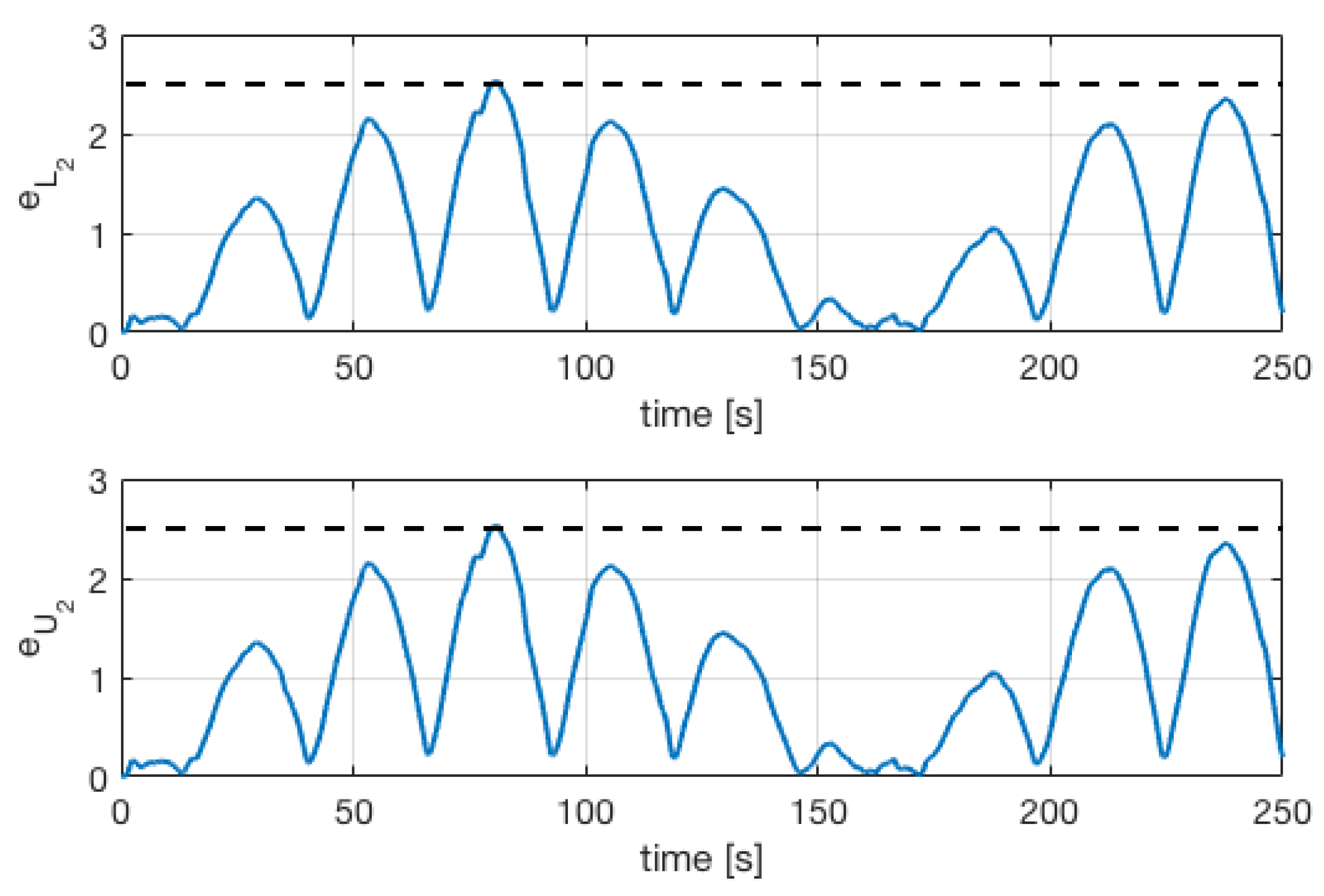
By following the FD-Algorithm stated in Algorithm 2, we need to define $T_h$ from the nominal case H, as stated in Table 1. We obtain Figure 3, where both errors (13) for this case are displayed. Then, we can define a threshold (third step of FD-Algorithm): $Th=2.5$ (this value can be obtained from Figure 3 or evaluating a bound for ${sup}_t\{e_{L_2}\left(t\right),e_{U_2}\left(t\right)\}$). 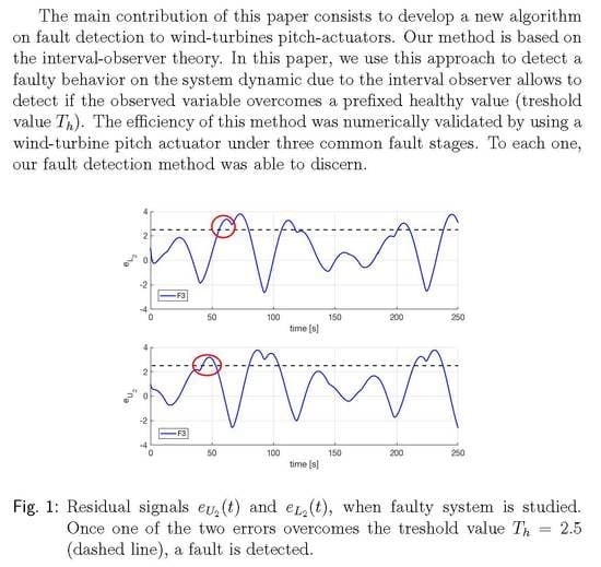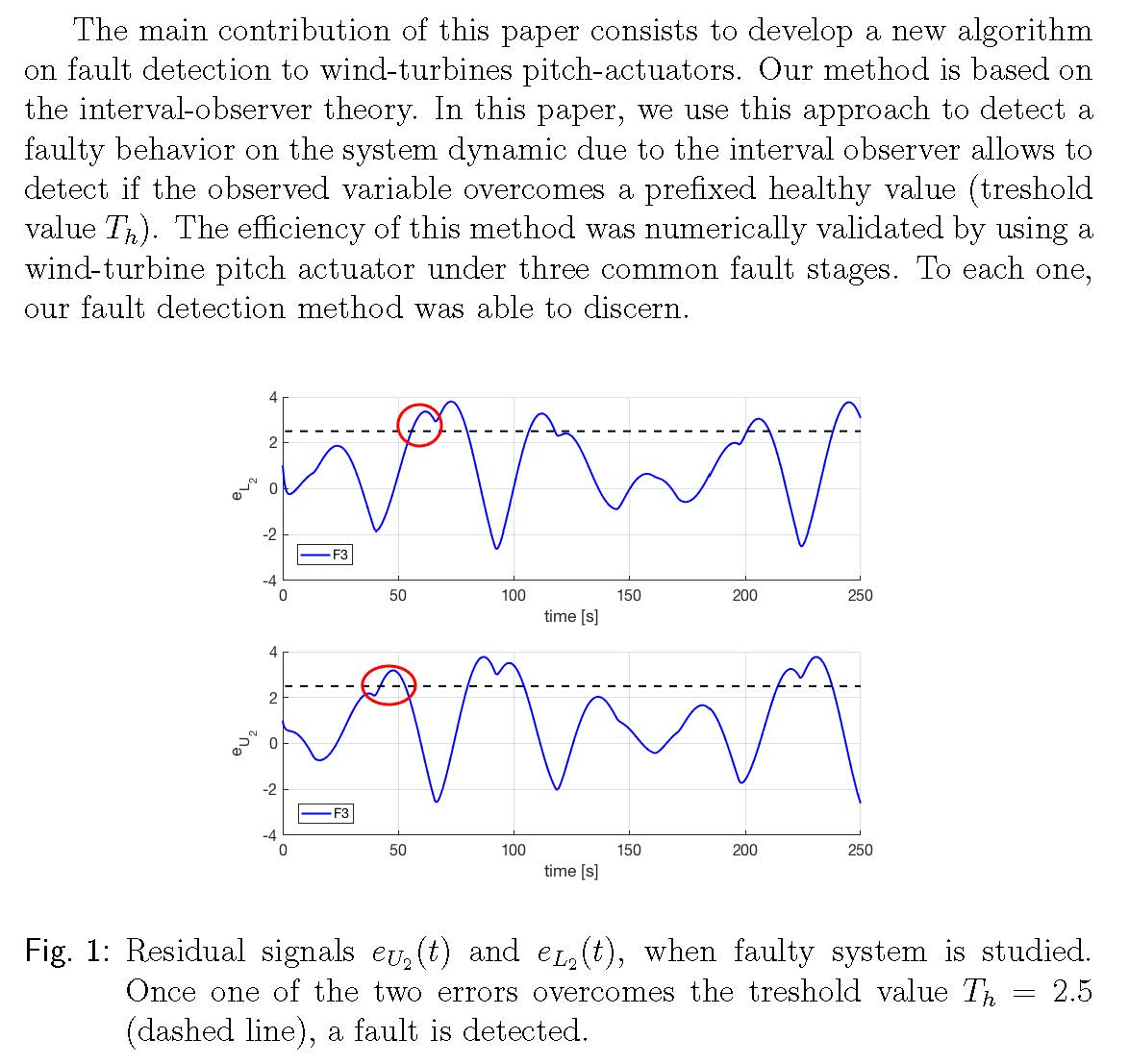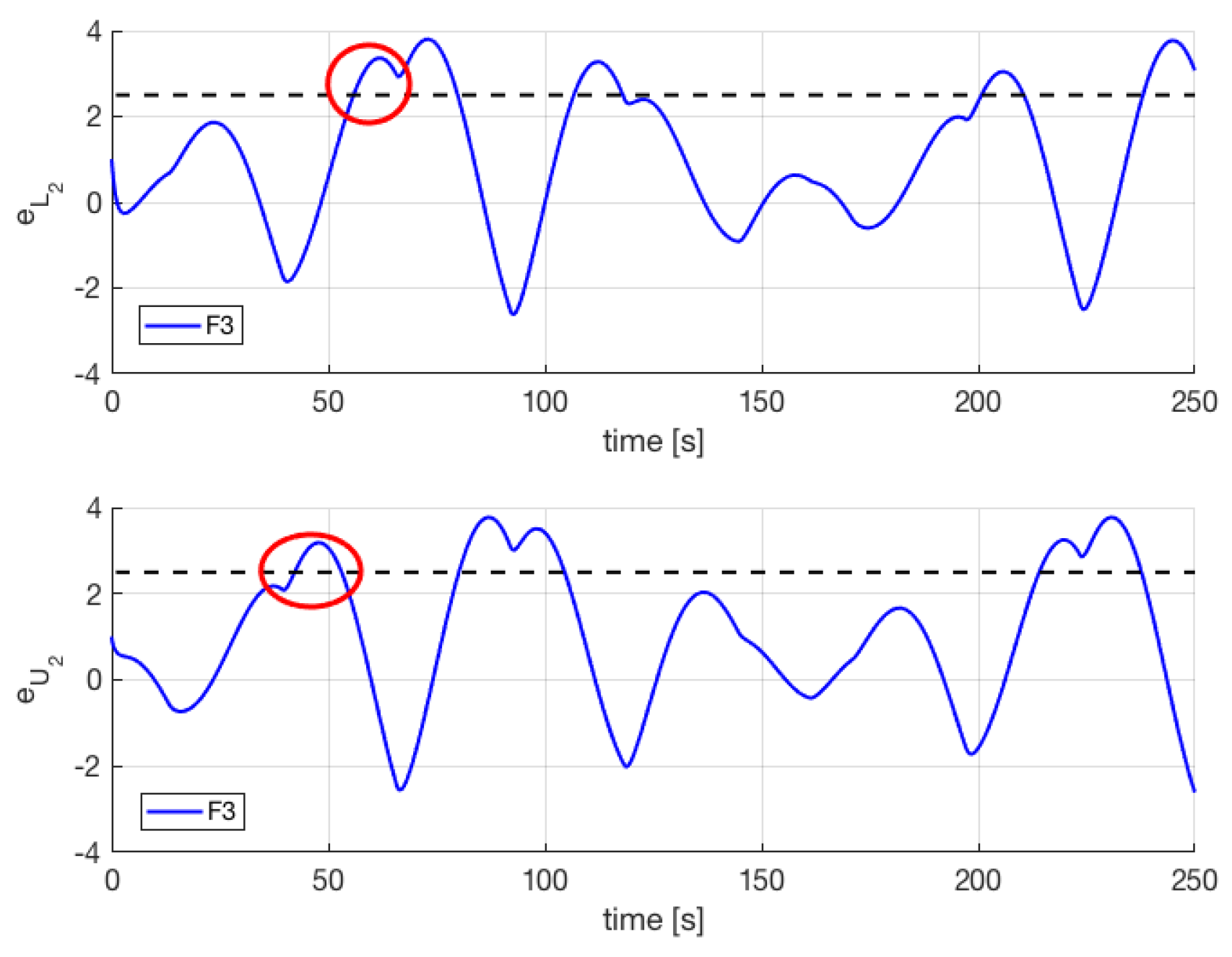Finally, we can use it to obtain a fault detection system (step 4 in Algorithm 2): faulty system (10) is considered and residual signals $e_{L_2}\left(t\right)$ and $e_{U_2}\left(t\right)$ are evaluated. The obtained simulation results for each faulty scenario are shown in Figure 4, Figure 5 and Figure 6. By using the stated excitation signal (or input signal), the occurrence of a fault is simple to realize: if ${sup}_{0\le t\le 250}{e}_{L_2}\left(t\right)\ge Th$, then a fault has occurred. Figure 4, Figure 5 and Figure 6 picture both errors (13), proving that it is necessary to consider $e_{L_2}\left(t\right)$ and $e_{U_2}\left(t\right)$ in Equation (13) to detect a fault because they do not detect a system fault at the same time. Thus, the designer has to evaluate (13) and the first to overcome $T_h$ detects a system fault.

Algorithm 2: Wind turbine fault detection algorithm (FD-Algorithm)

Step 1 Consider the healthy parameters shown in Algorithm 1, and then define matrix L (11). Step 2 Define a non-constant excitation signal $u\left(t\right)$. Step 3 From the nominal plant (H), define a threshold $Th$ as a bound to the system dynamic (13): 3.1 Solve (10) for $A_H$, $B_H$ and $L_H$ (12), along with (5) and (6). 3.2 Define a threshold $T_h$ to the dynamic in (13). Step 4 Decision rule. 4.1 Solve (10) for faulty A and B. 4.2 Solve (5) and (6), with $A_H$, $B_H$ and $L_H$ (12). 4.3 If residual signals (13) are greater than the set threshold $T_h$, then a fault is detected.

In Figure 3, the positiveness of the residual signal can be shown. When the faulty system is considered, the Metzler condition can be lost, so the non-negativeness of $e_U\left(t\right)\left(t\right)$ and $e_L\left(t\right)\left(t\right)$ in Equation (7) is not ensured. For instance, this can be noted in Figure 4, where both errors take negative values.

On the other hand, an important experimental issue is to evaluate how fast our detection system responds.

Table 2. Time estimation of the first detection by using the residual signals (13).

Scenario	${\mathit{t}}_{\mathit{U}}$ (seconds)	${\mathit{t}}_{\mathit{L}}$ (seconds)
High air oil content ($F_1$)	79.9382	58.0804
Hydraulic leakage ($F_2$)	31.3493	13.1228
Pump wear ($F_3$)	42.3287	55.9148

presents when the first fault is detected, for each case, and for both residual signals $e_{L_2}\left(t\right)$ and $e_{U_2}\left(t\right)$:

$$\begin{array}{c}{t}_L=\underset{0\le t\le t_f}{\min }\{e_{L_2}\left(t_L\right)>T_h\},\hfill \\ t_U=\underset{0\le t\le t_f}{\min }\{e_{U_2}\left(t_U\right)>T_h\},\hfill \end{array}$$

(14)

where $t_f$ is the total time of simulations.

Note that it takes less than a minute to detect a fault. In comparison to the technique stated, for instance in [20], our approach may be considered as a fast response method for detecting a fault. Moreover, from Figure 4 and Figure 5 and Table 2, a classification of a system fault can be stated, once the threshold value $T_h$ is defined. In a general scenario, once $e_{L_2}\left(t\right)$ or $e_{U_2}\left(t\right)$ are greater than the stated value $T_h$, a fault is detected. However, how may we classify it as $F_1$, $F_2$ or $F_3$? From Table 2, a response to this question can be inferred using (14). A classification algorithm is stated in Algorithm 3.

Algorithm 3: Fault classification algorithm (FC-Algorithm)

Step 1 Nominal plant: determine $T_h$. Step 2 General plant: Evaluate the first value of t (14) such that $e_{L_2}\left(t\right)$ or $e_{U_2}\left(t\right)$ (13) verify: 2.1 If $e_{L_2}\left(t\right)>T_h$ for $t\le 15$: then $F_2$ 2.2 If $e_{U_2}\left(t\right)>T_h$ for $15<t\le 55$: then $F_3$ 2.3 If $e_{L_2}\left(t\right)>T_h$ for $58\le t$: then $F_1$.

Finally, in real applications, even when we are actuating by using a known control signal to the pitch-actuator system of the wind turbine, there may exist a wind on the blades and then inducing of random dynamics on our structure. Hence, we repeat the previous simulations by adding a random signal to our control action as shown in Figure 7. The obtained results are shown in Figure 8, Figure 9, Figure 10 and Figure 11. From these figures, we see that the same fault detection algorithm is still possible.

To test the proposed FD-Algorithm (Algorithm 2) and FC-Algorithm (Algorithm 3), a set of 500 numerical experiments with random input data are carried out. The accuracy of the algorithms is displayed in

Table 3. Random sample test: Fault detection and classification percentage.

Fault Cases	F1	F2	F3
Detection	$62\%$	$80\%$	$91\%$
Classification	$83\%$	$100\%$	$100\%$

, where the percentage of right fault classification is over detected ones.

Comparing the achievement of the proposed algorithm related to others in literature [22,25], our approach is robust to noisy data, which would be a serious problem, for instance, to the fault detection technique in [25]. Thus, the image to process is obtained by reading a one-dimensional sensor in discrete-time domain. Moreover, our approach does not rely on accurate discrete-time modeling of the pitch system as the one stated in [22], for which its performance depends on the discrete-time sampling too. On the other side, among the different approaches on monitoring the mechanical structures on a wind turbine, there is the stochastic method focused to predict, for instance, vibrations at the tower top of wind turbine and fatigue loads due to the wind [15,16]. This stochastic approach resulted robustly against changing conditions and was able to separate the response dynamics of the system response from the deterministic one.

4. Concluding Remarks and Future Work

In this work, pitch actuator faults were studied due to these systems having the highest failure rate in wind turbines. A fault in a pitch actuator may change the dynamics of the pitch system by varying the damping ratio and natural frequencies from their nominal values, thus affecting the whole performance of a costly wind turbine. Thus, a fast and stable fault detection algorithm is an important key to study.

By using the interval observer theory, an original algorithm on fault detection to wind-turbine pitch actuators was successfully realized. This algorithm is based on knowing the healthy parameters of the plant. Then, we assume that, even if a fault occurs, the values of these parameters are not far away from the healthy one. Thus, we can consider an interval observer for a healthy region. Under a general scenario, from the residual errors, we can determine if the system fits this region or not. Thus, a fault detection system is obtained. On the other hand, in this paper, we focus on detecting faults on wind turbine pitch actuators. Therefore, the fatigue load damage estimation, and other wind-turbine structures’ metric performances, are not studied here. The efficiency of this method was numerically validated by using a wind turbine pitch actuator under three common fault stages. For each one, our fault detection method was able to discern. Moreover, the time response of our approach fault detection method can be considered fast.

As in [39], a Fourier theory can be used to study the principal harmonics of the residual signals. Comparing Figure 3 and Figure 8, where residual signals for healthy scenario are pictured, the behavior is almost the same. However, when a fault occurs, note that a a faulty system with a random component on the input signal presents more harmonics than the non-random one. Thus, as future work, a possible algorithm to detect a fault is to study the presence of harmonics in the residual signals by using the Fourier transform.

References

1. Hameed, Z.; Hong, Y.C.Y.A.S.; Song, C. Condition monitoring and fault detection of wind turbines and related algorithms: A review. Renew. Sustain. Energy Rev. 2009, 13, 1–39. [Google Scholar] [CrossRef]
2. Yin, S.; Wang, G.; Karimi, H. Data-driven design of robust fault detection system for wind turbines. Mechatronics 2014, 24, 298–306. [Google Scholar] [CrossRef]
3. Odgaard, P.F.; Stoustrup, J.; Kinnaert, M. Fault-Tolerant Control of Wind Turbines:A Benchmark Model. IEEE Trans. Control Syst. Technol. 2013, 21, 1168–1182. [Google Scholar] [CrossRef] [Green Version]
4. Xiao, C.; Liu, Z.Z.T.; Zhang, L. On Fault Prediction for Wind Turbine Pitch System Using Radar Chart and Support Vector Machine Approach. Energies 2019, 12, 2693. [Google Scholar] [CrossRef] [Green Version]
5. Gielen, D.; Boshell, F.; Saygin, D.; Bazilian, M.D.; Wagner, N.; Gorini, R. The role of renewable energy in the global energy transformation. Energy Strategy Rev. 2019, 24, 38–50. [Google Scholar] [CrossRef]
6. Delgado-Bonal, A.; Martín-Torres, F.J.; Vázquez-Martín, S.; Zorzano, M.P. Solar and wind exergy potentials for Mars. Energy 2016, 102, 550–558. [Google Scholar] [CrossRef]
7. Astolfi, D.; Castellani, F.M.L.A.; Terzi, L. Wind Turbine Systematic Yaw Error: Operation Data Analysis Techniques for Detecting It and Assessing Its Performance Impact. Energies 2020, 13, 2351. [Google Scholar] [CrossRef]
8. Lin, Z.; Liu, X. Assessment of Wind Turbine Aero-Hydro-Servo-Elastic Modelling on the Effects of Mooring Line Tension via Deep Learning. Energies 2020, 13, 2264. [Google Scholar] [CrossRef]
9. Byrne, R.; Astolfi, D.F.; Hewitt, N. A Study of Wind Turbine Performance Decline with Age through Operation Data Analysis. Energies 2020, 13, 2086. [Google Scholar] [CrossRef] [Green Version]
10. Barradas-Berglind, J.J.; Wisniewski, R.S.M. Fatigue load modeling and control for wind turbines based on hysteresis operators. In Proceedings of the IEEE 2015 American Control Conference, Chicago, IL, USA, 1–3 July 2015; pp. 3721–3727. [Google Scholar]
11. Wang, L.; Han, R.W.T.; Ke, S. Uniform Decomposition and Positive-Gradient Differential Evolution for Multi-Objective Design of Wind Turbine Blade. Energies 2018, 11, 1262. [Google Scholar] [CrossRef] [Green Version]
12. Lee, S.L.; Shin, S. Wind Turbine Blade Optimal Design Considering Multi-Parameters and Response Surface Method. Energies 2020, 13, 1639. [Google Scholar] [CrossRef] [Green Version]
13. Namik, H.; Stol, K. Individual blade pitch control of a spar-buoy floating wind turbine. IEEE Trans. Control Syst. Technol. 2013, 22, 214–223. [Google Scholar] [CrossRef]
14. Fitzgerald, B.; Staino, A.; Basu, B. Wavelet-based individual blade pitch control for vibration control of wind turbine blades. Struct. Control. Health Monit. 2018, 26, 1–12. [Google Scholar] [CrossRef] [Green Version]
15. Lind, P.; Herraez, I.W.M.; Peinke, J. Fatigue Load Estimation through a Simple Stochastic Model. Energies 2014, 7, 8279–8293. [Google Scholar] [CrossRef] [Green Version]
16. Lind, P.; Vera-Tudela, L.; Wächter, M.; Kühn, M.; Peinke, J. Normal Behaviour Models for Wind Turbine Vibrations: Comparison of Neural Networks and a Stochastic Approach. Energies 2017, 10, 1944. [Google Scholar] [CrossRef] [Green Version]
17. Gong, X.; Qiao, W. Current-Based Mechanical Fault Detection for Direct-Drive Wind Turbines via Synchronous Sampling and Impulse Detection. IEEE Trans. Ind. Electron. 2015, 62, 1693–1702. [Google Scholar] [CrossRef]
18. Badihi, H.; Zhang, Y.; Hong, H. Wind Turbine Fault Diagnosis and Fault-Tolerant Torque Load Control Against Actuator Faults. IEEE Trans. Control Syst. Technol. 2015, 23, 1351–1372. [Google Scholar] [CrossRef]
19. Liu, Z.; Xiao, C.; Zhang, T.; Zhang, X. Research on Fault Detection for Three Types of Wind Turbine Subsystems Using Machine Learning. Energies 2020, 13, 460. [Google Scholar] [CrossRef] [Green Version]
20. Lio, N.; Vidal, Y.; Acho, L. Wind Turbine Control and Monitoring; Springer: Berlin, Germany, 2014; Volume 121. [Google Scholar]
21. Ding, S. Model-Based Fault Diagnosis Techniques: Design Schemes, Algorithms, and Tools; Springer: Berlin, Germany, 2008. [Google Scholar]
22. Vidal, Y.; Tutiven, C.R.J.; Acho, L. Fault diagnosis and fault-tolerant control of wind turbines via a discrete time controller with a disturbance compensator. Energies 2015, 8, 4300–4316. [Google Scholar] [CrossRef] [Green Version]
23. Dong, J.; Verhaegen, M. Data driven fault detection and isolation of a wind turbine benchmark. In Proceedings of the IFAC World Congress, Milan, Italy, 28 August–2 September 2011; Volume 2, pp. 7086–7091. [Google Scholar]
24. Lan, J.; Patton, R.J.; Zhu, X. Fault-tolerant wind turbine pitch control using adaptive sliding mode estimation. Renew. Energy 2018, 116, 219–231. [Google Scholar] [CrossRef]
25. Ruiz, M.; Mujica, L.E.; Alferez, S.; Acho, L.; Tutiven, C.; Vidal, Y.; Rodellar, J.; Pozo, F. Wind turbine fault detection and classification by means of image texture analysis. Mech. Syst. Signal Process. 2018, 107, 149–167. [Google Scholar] [CrossRef] [Green Version]
26. Qiao, W.; Lu, D. A survey on wind turbine condition monitoring and fault diagnosis—Part I: Components and subsystems. IEEE Trans. Ind. Electron. 2015, 62, 6536–6545. [Google Scholar] [CrossRef]
27. Yang, W.; Tavner, P.; Wilkinson, M. Wind turbine condition monitoring and fault diagnosis using both mechanical and electrical signatures. In Proceedings of the 2008 IEEE/ASME International Conference on Advanced Intelligent Mechatronics, Xi’an, China, 2–5 July 2008; pp. 1296–1301. [Google Scholar]
28. Bolajraf, M.; Rami, M.; Helmke, U. Robust positive interval observers for uncertain positive systems. IFAC Proc. Vol. 2011, 44, 14330–14334. [Google Scholar] [CrossRef]
29. Ito, H. Interval observer of minimal error dynamics. Automatica 2020, 113, 1–6. [Google Scholar] [CrossRef] [Green Version]
30. Gouzé, J.-L.; Rapaport, A.; Hadj-Sadok, M. Interval observers for uncertain biological systems. Ecol. Model. 2000, 133, 45–56. [Google Scholar] [CrossRef]
31. Hadj-Sadok, M.; Gouzé, J. Estimation of uncertain models of activated sludge processes with interval observers. J. Process. Control 2001, 11, 299–310. [Google Scholar] [CrossRef]
32. Shu, Z.; Lam, J.; Gao, H.; Du, B.; Wu, L. Positive observers and dynamic output-feedback controllers for interval positive linear systems. IEEE Trans. Circuits Syst. I 2008, 55, 3209–3222. [Google Scholar]
33. Ellis, G. Introduction to observers in control systems. In Control System Design Guide; Elsevier: Amsterdam, The Netherlands, 2012; Chapter 10; pp. 185–212. [Google Scholar]
34. Hendel, R.; Khaber, F.; Essounbouli, N. Adaptive high-order sliding mode controller-observer for MIMO uncertain nonlinear systems. Asian J. Control 2020, 1–21. [Google Scholar] [CrossRef]
35. Chambon, E.; Apkarian, P.; Burlion, L. Metzler Matrix Transform Determination using a Nonsmooth Optimization Technique with an Application to Interval Observers. In Proceedings of the 2015 Conference on Control and its Applications, Paris, France, 8–10 July 2015; pp. 205–211. [Google Scholar]
36. Wan, Y.; Bevly, D.; Rajamani, R. Interval observer design for LPV systems with parametric uncertainty. Automatica 2015, 60, 79–85. [Google Scholar]
37. Nazir, M.; Khan, A.M.G.; Abid, M. Robust fault detection for wind turbines using reference model-based approach. J. King Saud Univ. Eng. Sci. 2017, 29, 244–252. [Google Scholar] [CrossRef] [Green Version]
38. Cho, S.; Gao, Z.; Moan, T. Model-based fault detection, fault isolation and fault-tolerant control of a blade pitch system in floating wind turbines. Renew. Energy 2018, 120, 306–321. [Google Scholar] [CrossRef]
39. Kalista, K.; Liska, J. Time-frequency methods for signal analysis in wind turbines. J. Phys. Conf. Ser. 2015, 659, 1–12. [Google Scholar] [CrossRef] [Green Version]
Figure 1. A schematic representation of the pitch actuator location in a wind-turbine.
Energies 13 02861 g001
Figure 2. Test input signal and state variables x 1 ( t ) and x 2 ( t ) for the healthy actuator response (with x 1 ( 0 ) = 0 and x 2 ( 0 ) = 0 ).
Energies 13 02861 g002
Figure 3. Observed errors or residual signals e U 2 ( t ) and e L 2 ( t ) for the nominal case H (see Algorithm 1). We can state T h = 2.5 as a bound for the residual signals (dashed). Note that both errors are identical because no fault is present.
Energies 13 02861 g003
Figure 4. Fault F1 scenario. Residual signals e U 2 ( t ) and e L 2 ( t ) . Once one of the two errors overcomes the dashed line, a fault is detected.
Energies 13 02861 g004
Figure 5. Fault F2 scenario. The first fault detection for both residual signals or observed error is in red.
Energies 13 02861 g005
Figure 6. Fault F3 scenario. In this case, the residual signal e U 2 allows for detecting a fault faster than e L 2 .
Energies 13 02861 g006
Figure 7. Top: Input signal with random noise; Down: variables of wind turbine system (10).
Energies 13 02861 g007
Figure 8. Residual signals e U 2 ( t ) and e L 2 ( t ) for the nominal case H when a random noise is present on the input reference signal, similar to non-random input (see Figure 3). Again, the programmed threshold is T h = 2.5 (dashed).
Energies 13 02861 g008
Figure 9. Fault F1 scenario under a random noise. Residual signal e U 2 detects a faulty behavior due to high air oil content, despite noise on the input signal.
Energies 13 02861 g009
Figure 10. Fault F2 scenario under a random noise, with similar behavior of non-random input case (see Figure 5).
Energies 13 02861 g010
Figure 11. Fault F3 scenario under a random noise. Note that e L 2 > T h before e U 2 , but the same non-noisy classification rule still works because cases 2.1 or 2.3 in FC-Algorithm are not accomplished.
Energies 13 02861 g011