1. Introduction
The reactive power dispatch (RPD) problem is a sub problem of optimal power flow (OPF). The optimal solution for the RPD problem has extensive control over stability, security, and cost-effective operation of the whole power system. By and large, reactive power generation in a system is altered to improve its voltage stability. While reallocating the reactive power, care should be taken that the transmission losses incurred are also minimum. It follows that, in order to obtain the optimum reactive power dispatch, the problem should minimize two objective functions: (i) Transmission loss and (ii) voltage deviation. The voltages of load buses can be considered to indicate the voltage stability of the system by keeping themselves within the stipulated tolerance limit. The RPD problem determines the control variable values for which the power losses occurring during transmission will be the minimum. The design variables for the RPD problem are reactive power compensator outputs, voltages of generator buses, and tap ratios of transformers. The RPD is a non-linear, non-convex optimization problem classified as a mixed-integer discrete continuous (MIDC) problem as it handles continuous, integer, and discrete control variables.
Research in bygone years utilized conventional methods [
1,
2,
3] chiefly to solve the RPD optimization problem. Conventional methods worked on the problem after performing suitable mathematical assumptions, thus reducing the computational complexity of the RPD problem. With the use of interior point (IP) methods [
4], the computational burden could be reduced considerably. The additional advantages offered by IP methods include fast convergence and convenient handling of inequality constraints. Akin to IP methods, non-linear [
5] and quadratic programming methods [
6] have also been used for solving the problem, but seemed to be unproductive at handling the multiplicity in design variables. The RPD problem particularly involves control variables of all types—continuous, discrete, and integer. As the results brought about by all the techniques investigated so far provided only continuous values, the solutions had to be rounded off for implementation. The shortcomings of such rounding-off methods have been enlightened in [
7]. One of the three major concerns of Tinney et al., as explained in [
7], is the determination of a feasible and optimal solution for problems containing integer, discrete, and continuous variables. A creative suggestion put forth by them is the application of heuristic methods that are capable of giving quick and more accurate solutions to such problems. The application of evolutionary programming methods that have intrinsic skill to determine the near-global optimum solution forms the second generation of solution techniques [
8,
9,
10,
11]. Methods such as genetic algorithm (GA) and particle swarm optimization (PSO) and many other hybrid varieties fundamentally build upon them and have opened up an altogether new era for solving the combinatorial problems in numerous fields [
12,
13,
14,
15,
16]. Heuristic methods are distinct from conventional methods for that matter as they possess the ability to drive the solution to the nearest possible optimal solution point, thereby escaping convergence to local minima at an early stage, but the solutions obtained are all continuous whatever the kind of variable. The results for discrete, as well as integer, variables are then rounded off to make them hardware-feasible, and then a final solution is obtained considering the actual continuous variables alone. Such newly obtained solutions may be quite trivial and far from optimal, if not unfeasible, thus disturbing the stability of the system. One of the commendable research studies for finding out the optimal solution for such problems has evolved into a method that considers discrete variables as continuous in the initial steps and alters the objective function with a suitable penalty function addition [
17]. The methodology definitely provides good results; however, inclusion of an apt penalty function adds to the complexity of the problem. Moreover, utmost care should be taken while choosing the penalty function to avoid creating any adverse effects in the objective function value. The penalty functions used by the researchers to solve the problem were claimed to be tailored in specific ways to suit a particular problem and a particular set of variables. Such special functions could not be used in general for other problems. Thus, a simple and efficient method to solve MIDC problems like RPD is yet to evolve.
Many newly developed meta-heuristic algorithms like ant-lion optimizer [
18], dragon fly optimization [
19], hybrid particle swarm optimization–Tabu search (PSO–TS) [
20], and hybrid artificial physics optimization–particle swarm optimization (APOPSO) [
21] have been put forth to solve the RPD problem. Though all are found to be efficient methods to achieve the main objectives, none of them specifically calculate the discrete variables as discrete and integer variables as integer during the solution determination process. The solution obtained by these methods has to be rounded off to be feasible for discrete and integer hardware elements, which may bring about loss of optimality of the solution. Hence, it has become quite essential to determine an effective method that would solve the RPD problem in such a way that the solution obtained directly gives implementable values for discrete and integer variables, just as for continuous variables. A method for finding out the optimum solution by treating integer and discrete variables as such from beginning to end of the solving process would definitely deduce a fruitful solution with feasible and practicable values for all the different kinds of variables.
1.1. Hypothesis
Diversity-enhanced PSO (DEPSO), an improvisation to the basic PSO, proposes itself to be capable of providing the required result. The scheme is based on the three-phase particle evolution law and is quite effective in breeding the best possible solution. The method considers all three different kinds of variables as such from the start of the solving procedure and maintains their nature throughout the problem solving process. Moreover, the merits of the method include simplicity, efficiency, and non-usage of complex and problem-specific penalty functions. To the best knowledge of the authors, DEPSO has not yet been applied to the RPD problem.
1.2. Objectives
The objective of the present work is to investigate the effectiveness of implementing the DEPSO algorithm to the RPD problem. The DEPSO algorithm has been successfully experimented on IEEE 14-, 30-, and 118-bus test systems, and the results are compared to those obtained using basic PSO and JAYA algorithms. It must be mentioned that the proposed method proves to be an effective strategy for determining the optimal reactive power dispatch by providing excellent results with implementable values for all the different control variables and optimal values for the objective functions. Further, the same method has been used to calculate the reactive power dispatch for a system on a twenty-four-hour basis to establish the capability of the method for application to dynamic reactive power scheduling.
2. Problem Formulation
The objectives of the work are minimization of real power transmission losses in the system and minimization of total bus voltage deviation. The control variables under consideration are the PV bus voltages (), ratios of transformer taps (), and shunt compensator reactive power outputs (). Values for the control variables that bring about the desired results are different for different formulations. The present work can be mathematically expressed as three formulations.
Formulation 1: Minimization of real power losses.
Find
to reduce the transmission losses to a minimum.
where
is the sum of real power losses in all lines.
is the penalty function defined by Equation (3),
Vi,
Vj are the bus voltage magnitudes at buses
i and
j, respectively,
θij is the phase angle difference between
Vi and
Vj in radians,
Gk is the conductance of branch
k, and
are penalty factors, chosen in such a way that the reactive power generation limit violations and line flow limit violations are properly accounted for.
Formulation 2: Minimization of load bus voltage deviations.
Find
to reduce the load bus voltage deviations from the reference value to a minimum.
The reference voltage considered is and is the load bus voltage.
Formulation 3: Minimization of real power losses and total bus voltage deviations.
Find
to reduce the load bus voltage deviations from the reference value to a minimum.
where
Here, the multi-objective RPD problem is formulated by the weighted sum approach, by assigning suitable weights to both the objective functions. represents the combined objective function, denotes the objective function due to total real power transmission loss incurred in the system, and implies the objective function corresponding to the deviation in per-unit voltage of the load buses in the system. The weight is chosen to vary from 0 to 1 in steps of 0.1.
System Constraints
The equality and inequality constraints to which the problem is subjected are given as follows:
P,
Q,
V,
T,
S,
G, and
B respectively denote real and reactive powers, voltage, transformer tap, thermal limit of transmission line, conductance, and susceptance. Subscripts
B,
BR,
g,
d,
c,
load,
loss,
lb, and
l correspond to bus, branch, generator, demand, compensator, load, loss, load bus, and line, and indices
i,
j,
k, and
m represent the number of the generator, load, bus, and transformer or line as the case may be. Power balance equations and generator reactive power limits are taken care of during load flow. The limits of transformer tap and compensator output are encompassed in the feasible solution set. The bus voltage and line flow limit constraints are added to the objective function with the necessary static square penalty function for limit violations as follows:
3. Mathematical Modeling of the System
Generators in the test systems are modelled as voltages behind reactances, transformers as series reactances, and loads as PQ models, and transmission lines are represented by their π models. Load flow analysis is done by using the Newton–Raphson method. Reactive power can be provided with the aid of any shunt flexible alternating current transmission system (FACTS) device kept at the corresponding bus. In this work, the static synchronous compensator (STATCOM) has been used to supply the necessary reactive power at strategic locations by injecting shunt current into the network with the aid of an injection transformer. As the device is capable of supplying the required amount of reactive power in quadrature with the line current, the real power transfer between a lossless STATCOM and system is practically zero. Thus, it can be modeled [
22] by the following equations:
where
is the ac voltage at the output of STATCOM, referred to as the
system bus to which it is connected.
is the reactive power exchange for the STATCOM with the bus.
4. Solution Methodology
The reactive power dispatch problem has been solved by using three methods, the conventional PSO, JAYA algorithm, and diversity-enhanced PSO. A detailed comparison of results obtained from the three methods in terms of real power, reactive power, and execution time is carried out to analyze the performance of the algorithms. The solution methodologies are explained in this section.
4.1. Particle Swarm Optimization
One of the widely used simple and effective techniques for the solving of complex non-linear problems is the particle swarm optimization (PSO), proposed by Eberhart and Kennedy in 1995 [
23]. Fundamentally, PSO emulates the search process for food articulated by fish schools or bird swarms, hence developing its specific name. The global optimum point is determined as the particles (fish or bird) move around in the search space. Dimensions of solution space are decided by the number of variables of the problem. The velocity and position of each particle are updated iteratively to push them toward a global optimal solution. The velocity and position of each particle are modified as follows:
where inertia weight, and iteration and particle number are
w,
k, and
i, respectively, and
v and
x are velocity and position, respectively.
c1 and
c2 take care of the challenges in local, as well as global, search, and
ζi and
ξi are two random numbers. Pbest
i is the best previous position and gbest is the best particle among the group. Constriction factor
χ is a function of
c1 and
c2 given by:
where
and
. The inertia weight is given by:
where
is the value of inertia weight at the beginning of the iterations,
is the value of inertia weight at the end of the iterations,
is the current iteration number, and
is the limiting number of iterations. Suitable selection of the inertia weight provides good balance between global and local explorations. The particle velocity has been maintained between 0.03 and −0.03.
4.2. Diversity-Enhanced Particle Swarm Optimization
When a swarm of particles move together in a solution space in an uncontrolled manner, there is always a possibility of local accumulation and, hence, of a premature convergence due to congestion between the particles. Diversity-enhanced PSO (DEPSO), a modification to the fundamental PSO, put forth by Chun et al. [
24] in 2013, provides a very effective strategy for handling the mobbing of particles. The importance of preserving the diversity between candidate heuristic solutions in PSO, as well as GA, is explained in [
25,
26]. DEPSO allows the programmer to use an easy technique to solve MIDC problems without adding any extra factors or penalty functions. RPD is categorized as a MIDC problem, with the reactive power compensator output as an integer variable and transformer tap settings as a discrete variable. In this work, DEPSO is employed to solve the RPD problem. The control/decision variable vector for the problem is defined as:
where
are vectors of continuous, discrete, and integer variables. The vector
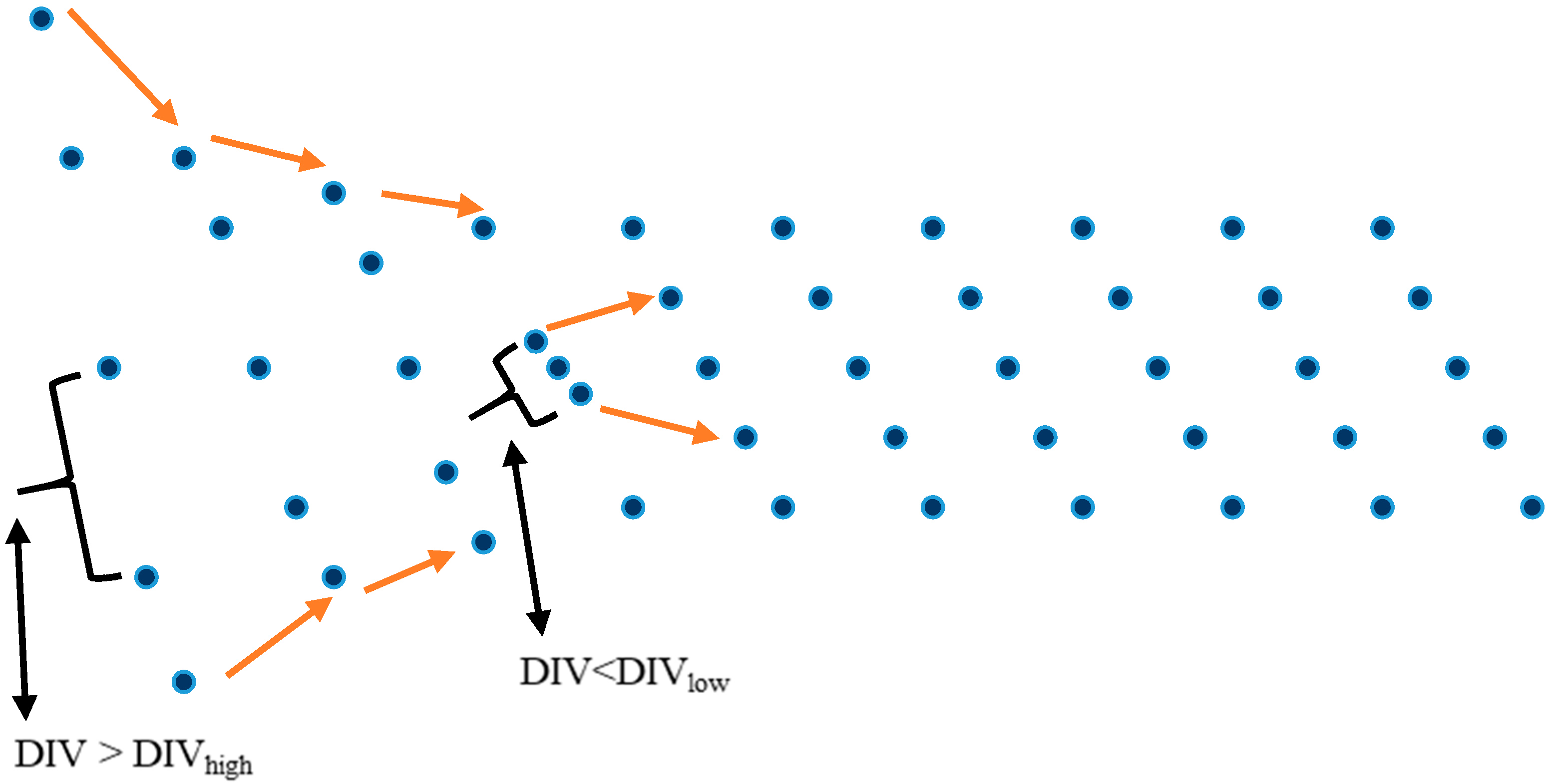
forms the solution vector. The method avoids the chances of particles getting stuck in local minima, thus rejecting the likelihood of untimely convergence. The particle movement in solution space includes three phases, as mentioned by Pant et al. [
27] in 2007, viz., phase of repulsion and attraction, and a phase between the two. The distance between particles is a measure of the diversity. When the diversity factor,
DIV, is higher than an upper bound
DIVhigh, the particles are attracted to each other. Further, if they come too near with
DIV less than the lower threshold limit
DIVlow, the particles enter a repulsion phase. The characteristics of the particles between the two phases are those of uniform motion. In this phase, the attraction suffered by its own previous best position for each particle is equal to the repulsion from the best known particle position in the group. The corresponding equations are:
The mean of Euclidean distances of all candidate variable values from the average point is the diversity factor.
where the number of particles is denoted as
mp and the number of variables is represented as
nv.
c1 and
c2 are the cognitive scaling factor and social scaling factor, respectively. Other notations are identical to those of basic PSO. The values of
DIVhigh and
DIVlow depend on the problem and are carefully chosen after several trials in order to avoid both scattering of particles, as well as premature convergence.
Figure 1 shows the movement of particles in the DEPSO method.
The pictorial representation depicts the movement of five particles along the positive X-axis direction. Initially, they are far away from each other. As the diversity between them is higher than the upper threshold value, as depicted in the figure, a suitable velocity step is given to reduce it. When, at some point of movement, the diversity is found to be less than the lower threshold, the particles move away from each other to maintain necessary diversity. The DEPSO algorithm is proficient and easy to implement.
DEPSO Algorithm
Step (1) Initialize particle (set of decision variables) position, velocity.
Step (2) Perform load flow study to find out the objective function (sum of active power loss and voltage deviation).
Step (3) Evaluate the penalty values with respect to the inequality constraint violations.
Step (4) Calculate fitness function for all particles.
Step (5) Decide and keep aside pbest and gbest.
Step (6) Calculate the diversity factor of the particles and update the velocity vector using the three-phase law.
Step (7) If the diversity factor is more than its upper threshold value, update the velocity with the equation for attraction phase, and if it is less than its lower threshold value, update with the equation for repulsion phase; otherwise update with equation for the phase of positive conflict.
Step (8) Check whether the maximum velocity step limit has been violated.
Step (9) Update the position of the particle with new velocity.
Step (10) Perform load flow investigation with the updated set of particles to obtain the objective function and calculate the fitness function by adding suitable penalties for inequality constraint violation.
Step (11) If the objective function is less than the previous value, update pbest and gbest.
Step (12) Repeat steps 6 to 11 until the termination criterion is reached.
Algorithm 1 below provides the pseudo-code for the proposed DEPSO method used for solving the reactive power dispatch problem. The optimal values of control variables are finally available in gbest so that it can be directly used for implementation in the particular system under consideration.
| Algorithm 1 Pseudo-code for DEPSO |
| For each particle |
| 1. Initialize all variables (swarm) |
| 2. Perform load flow analysis to find objective function |
| 3. Calculate fitness function by accommodating constraints |
| Decide pbest and gbest |
| While iter < itermax |
| For each particle |
| 4. Calculate diversity factor |
| 5. Update velocity according to diversity factor based on three phase law |
| 6. Check whether maximum velocity step limit has been violated; if so, limit it at maximum. |
| 7. Update particle position with the new velocity |
| 8. Perform load flow and calculate fitness values |
| 9. Update pbest and gbest if fitness values are better |
| End while |
4.3. JAYA Algorithm
The JAYA algorithm is a recently established, simple algorithm appropriate for unconstrained, as well as constrained, optimization problems [
28]. Though the JAYA algorithm is fundamentally very similar to PSO in generating an initial random solution to the control variables, it builds upon itself by moving toward the best solution, repelling away from the worst solution. In addition, no penalty function or factor is being introduced for the particles to be forced to reach the solution. Hence, this search method is quite suitable to be compared to the proposed DEPSO method. Initially,
random solution sets are generated, for
decision variables. The load flow program is run using the decision variable values. The objective function is evaluated and fitness value is calculated for each solution set. The solution corresponding to maximum fitness (best value of the objective function) is referred to as the best solution and that relating to minimum fitness (worst value of the objective function) is marked as the worst solution. The solution set is updated using the equation given by (25). The update is based on the concept that while stirring toward the best solution, the algorithm overlooks discontent simultaneously moving far away from the worst solution. The best and worst solution vectors are updated after each iteration. ‘JAYA’ is the Sanskrit word for ‘victory’ or ‘success,’ and the algorithm, even without any specific parameters, determines the optimum solution. The value of the updated solution
is
where
is the number of iterations,
and
are two random numbers within [0,1],
is the best value, and
is the worst value of the solution variable vector until the
th iteration. The random numbers can be chosen as scalars or vectors according to the requirement of the problem and can be allowed to change or be prefixed within a specific limit according to the discretion of the programmer.
5. Implementation in Test Systems
MATLAB coding for the RPD solution has been done separately using PSO, DEPSO, and JAYA algorithms. The effectiveness of DEPSO over PSO and JAYA RPD algorithms is assessed by testing it on standard IEEE 14-, 30-, and 118-bus test systems. The upper and lower bounds of all the three sets of control variables are listed in
Table 1. The values of transformer tap settings vary in discrete steps of 0.02 p.u.
Test Systems
Case studies have been conducted using the three algorithms in three standard IEEE test systems. The parameters of the test systems, which are used to conduct the simulation in an efficient manner, are presented in
Table 2 below. According to the data available online, the 14-bus system has provision to accommodate one reactive power source at bus no. 9, the 30-bus system has three compensators at buses 3, 10, and 24, and the 118-bus system has 14 reactive power source locations. Simulation and analysis are done according to the structure of the test systems available with the IEEE data set [
29].
6. Simulation Results and Discussion
In order to express the supremacy and effectiveness of the proposed method, many tests have been conducted on IEEE 14-, 30-, and 118-bus test systems. Most of the published literature on the RPD problem illustrates work on these test systems. The tests were carried out on a personal computer with an Intel® Core™2 Duo processor working at 2.24 GHz and 2 GB of RAM memory. The simulation has been performed using codes written in MATLAB R2014a for the specific algorithms in conjunction with MATPOWER 3.2.
6.1. IEEE 14 Bus System
The IEEE 14-bus system consists of five automatic voltage regulator (AVR)-controlled generators, 9 load buses, 20 branches, and three on-load tap changing transformers kept at lines (4,7), (4,9), and (5,6). The reactive power source is kept at bus-9. At initial operating conditions, the system real power losses are found to be 13.546 MW. The number of decision variables chosen for the IEEE 14-bus test system is 9. Hence, the search for the finest solution is done in a nine-dimensional search space. A comparison of the optimal values of the system decision variables obtained by solving the RPD with the proposed DEPSO, PSO, and JAYA algorithms has been tabulated in
Table 3.
From
Table 3, it can be seen that DEPSO is able to search and find the exact values for integer and discrete variables along with continuous variables in the continuous multidimensional search space.
While PSO and JAYA algorithms yield continuous values for all variables, whose values are to be rounded off for implementation, the DEPSO method provides the exact tap setting values and integer reactive compensator outputs as given by hardware constraints. Close examination of the table brings to any one’s attention the fewer losses incurred during the execution of RPD with DEPSO results. In all the three formulations considered, the results for the diversity-enhanced PSO is highlighted.
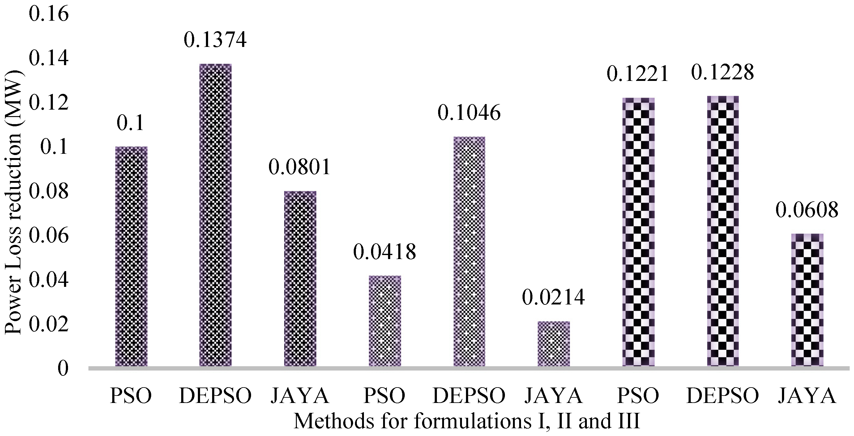
A column chart showing power loss reduction in all the nine cases is shown in
Figure 2.
The real power loss amounts to 13.4086 MW, resulting in a reduction of 0.1374 MW when the RPD with the DEPSO method is used with formulation I, i.e., minimization of real power losses alone is considered as an objective function. The chart also reveals that power loss reduction is higher for the DEPSO-based results in the other two formulations. Percentage power loss reduction is found to be maximum in the case of DEPSO, i.e., 1.01% for formulation I, 0.77% for formulation II, and 0.91% for formulation III. Hence, it may be established that the proposed method is superior over PSO and JAYA methods in the case of the reactive power dispatch problem to obtain the most optimal and feasible solution.
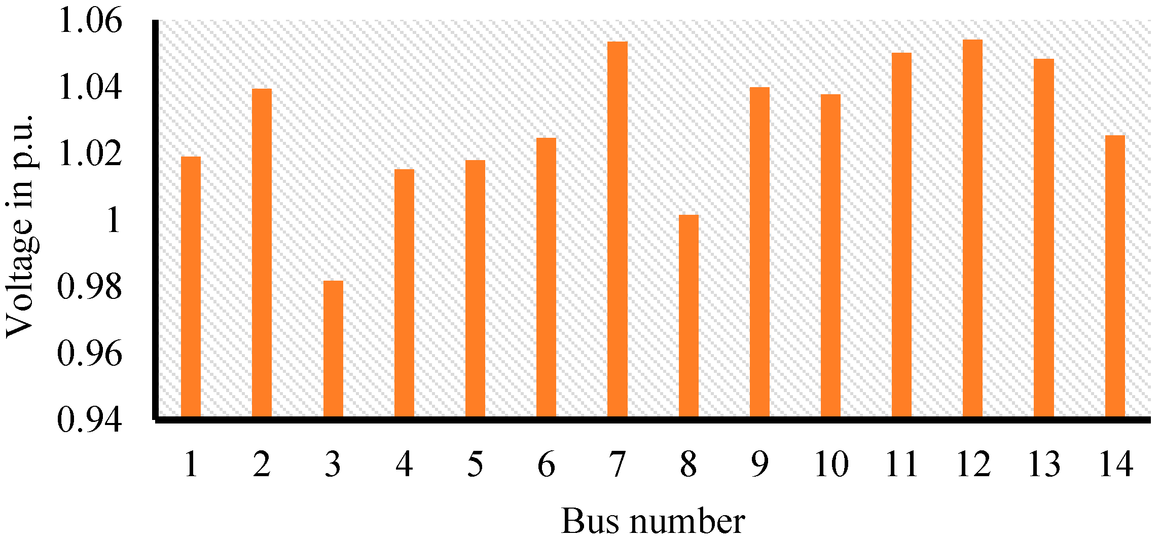
As the bus voltages are subjected to changes during load flow and has to be maintained within the upper and lower bounds, the voltage profile of all 14 buses in the system was checked and found to be within the limits, as clearly indicated in
Figure 3.
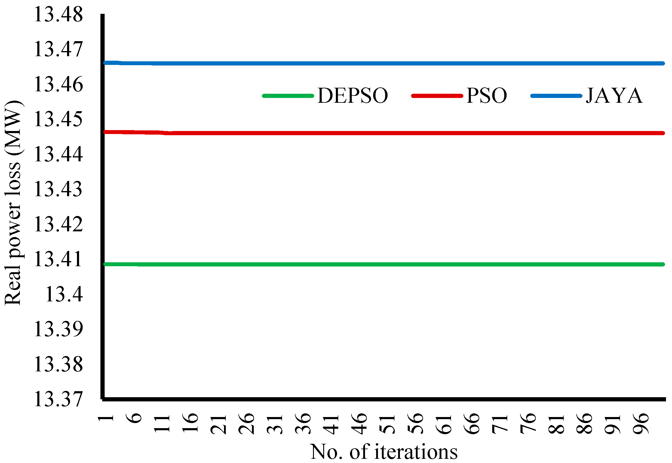
The convergence plot of
Figure 4 gives a visual presentation of the manner in which the real power losses reduce iteratively. DEPSO, PSO, and JAYA methods converge to the optimum value of the objective function respectively at the 9th, 11th, and 12th iterations. Thus, it can be accepted that the proposed method yields results at a competently fast rate.
6.2. IEEE 30-Bus System
The IEEE 30-bus test system consists of six generators and four transformers installed at (6,9), (6,10), (4,12), and (27,28) lines. The shunt compensators are provided at buses 3, 10, and 24. Values of control variables that lead to the optimum value of the objective function in various cases for the IEEE 30-bus test system are arranged in
Table 4.
Table 4 indicates that the DEPSO method produces integer results directly for integer variables and discrete values, which are feasible according to the hardware limitations for transformer tap settings. At initial operating conditions, the system losses are found to be 17.557 MW. The real power loss incurred with DEPSO-based results are less than those of the other two methods in all the three formulations. The time taken for each of the algorithms as presented in the table reveals that the DEPSO algorithm is faster than PSO and JAYA, thus making it a potential candidate for any application.
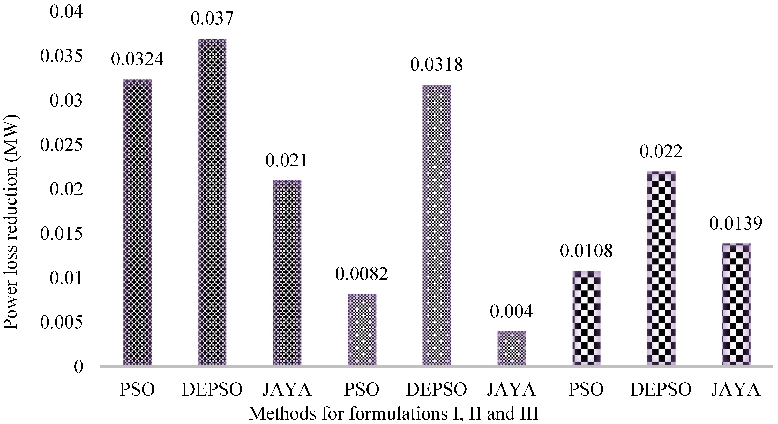
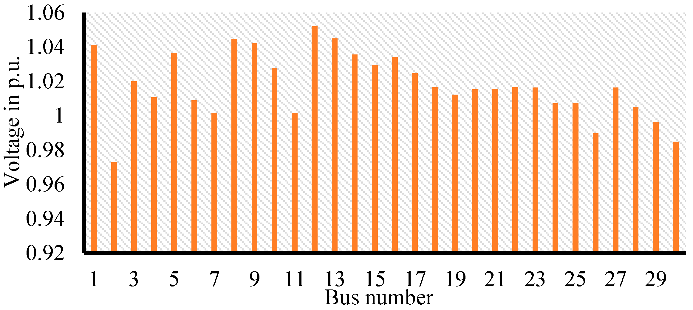
Figure 5 represents the power loss reduction obtained by the different methods under different formulations of the RPD problem. In formulation I, DEPSO leads the scoreboard with 0.21% power loss reduction. In formulation II, the DEPSO-based result provides 0.18%, whereas the PSO and JAYA algorithms provide 0.04% and 0.02% power loss reductions, respectively. Formulation III results show that DEPSO gives a power loss reduction 7% more than that of PSO and 5% more than that of JAYA methods. It can be explicitly stated that DEPSO in all the cases brings about solutions that cause maximum power loss reduction. The voltage profile of the IEEE 30-bus system after solving the multi-objective function using DEPSO is shown in
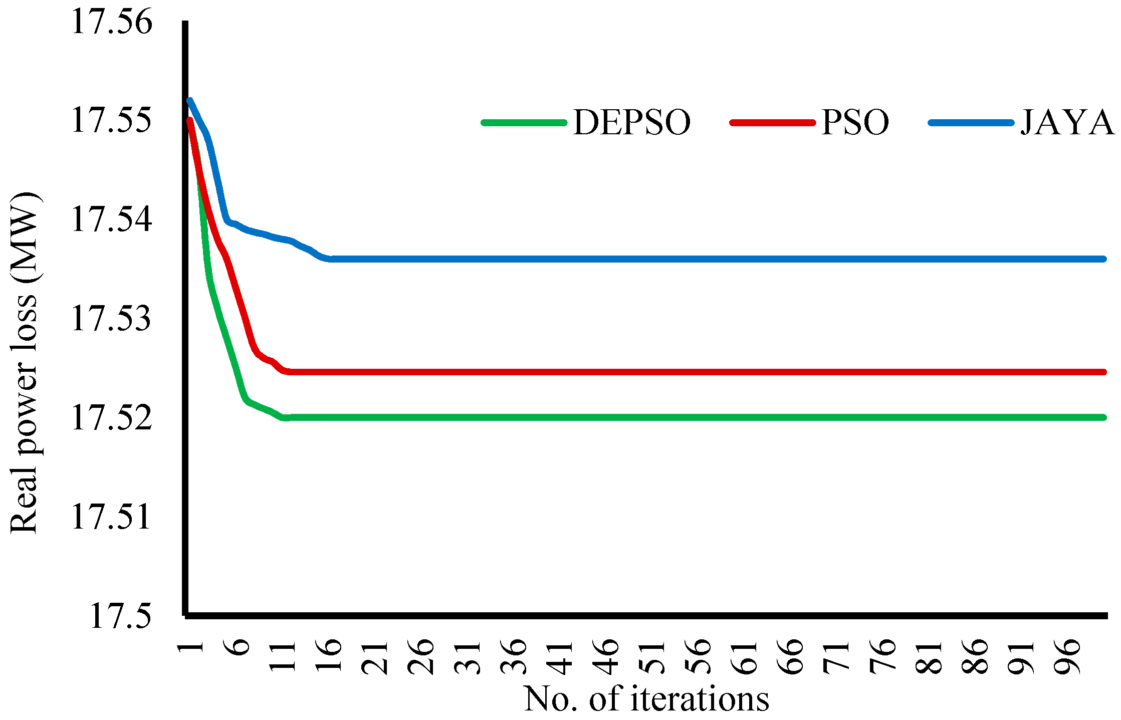
Figure 6. All the bus voltages are found to be within the limits specified. Convergence of the objective function for formulation I, i.e., real power loss minimization for 30-bus test system, is shown in
Figure 7. DEPSO, PSO, and JAYA methods converge at the 11th, 12th, and 16th iterations, respectively. Considering the speed of convergence also, DEPSO proposes itself to be a good method.
6.3. IEEE 118-Bus System
The test system consists of 54 generators, 9 transformers, and 14 reactive power sources kept at specific locations. The transformer taps as in the other test cases could be set at any one of the values {0.95, 0.97, 0.99, 1.01, 1.03, 1.05}. Out of the 77 decision variables of the system, all the 9 transformer tap positions are obtained as discrete values and 14 reactive power compensator outputs as integer in nature at each instant of time during the course of optimization solution determination.
The optimal values of the discrete and integer control variables of the test system as obtained using all the three methods for all three formulations are summarized in
Table 5. All the generator bus voltages, however, have been obtained in all cases as continuous values and are found to be within limits. The values of 54 generator bus voltages are tabulated as
Table A1 in
Appendix A. The reactive power compensator output takes integral steps. The advantage of the proposed method is that hardware constraint information of transformer tap settings can be incorporated and regularly checked at each iteration before arriving at the optimal solution. The proposed method also computes integer values for reactive power injections at various buses, satisfying all the constraints given by Equations (7)–(13) and, at the same time, maintaining the transmission line losses to a minimum level. The supremacy of the proposed method is demonstrated by comparing the results to those obtained by PSO and JAYA techniques. Unpredictability of the initial solution is taken care of by executing the simulation 50 times for all three methods. The values of power loss reduction expressed in MW is a direct measure of the additional benefit of the new method, diversity-enhanced PSO, which fundamentally renders a solution containing discrete values for discrete variables and integer values for integer variables along with continuous variables.
At initial operating conditions, system losses are found to be 133.101 MW. The transmission line losses computed from the simulation results and as given in
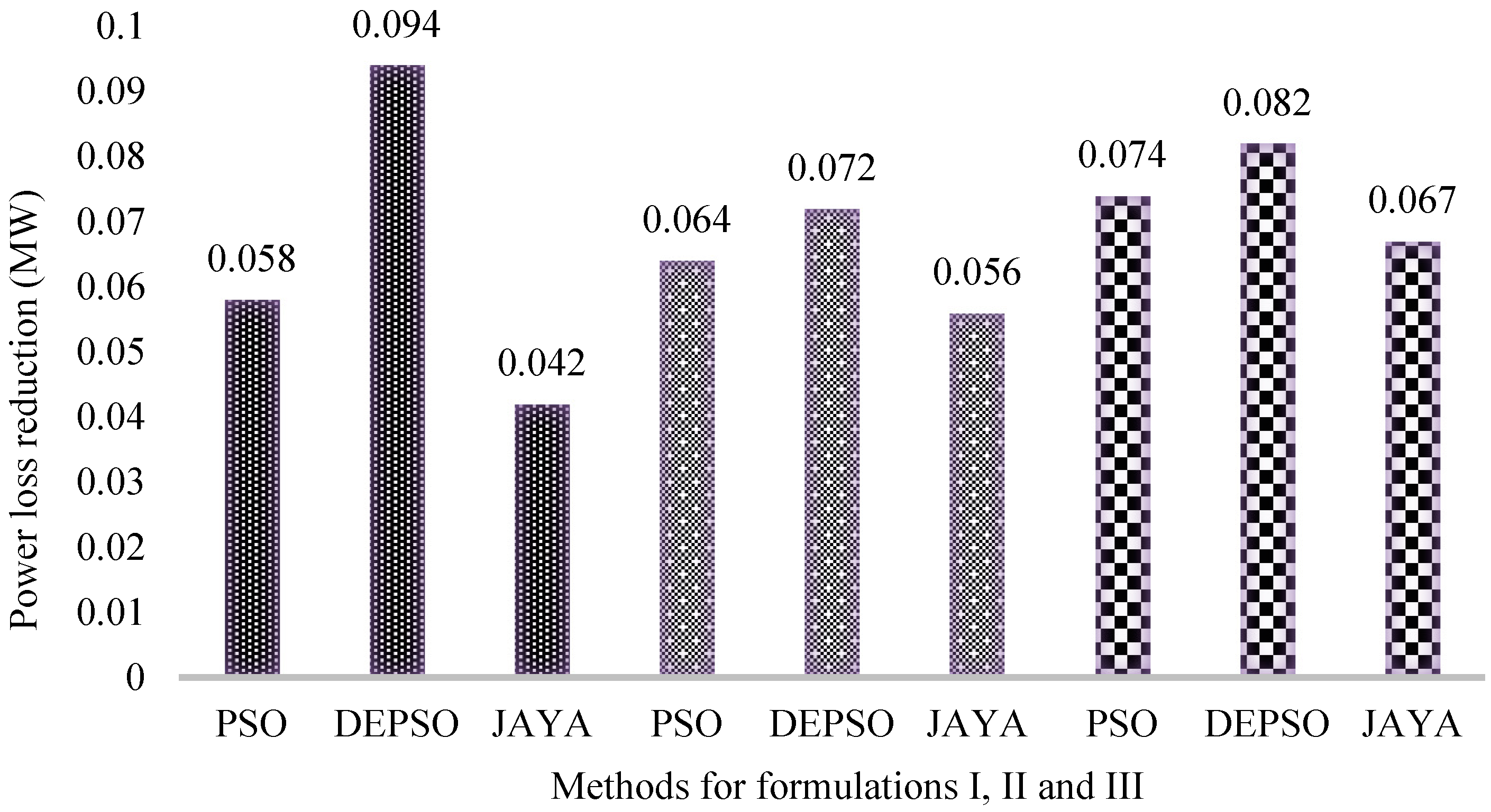
Table 5 indicate that using the proposed DEPSO method, power loss reduction can be improved compared to PSO and JAYA methods. A comparison of the power loss reduction made by all three methods is given as a bar graph in
Figure 8. The percentage power loss reduction provided by the proposed method is much more than those given by the other two methods in all three formulations for the IEEE 118-bus test system. DEPSO contributes a 0.7%, 0.5%, and 0.6% power loss reduction in formulations I, II, and III, respectively, whereas other methods provide lower values.
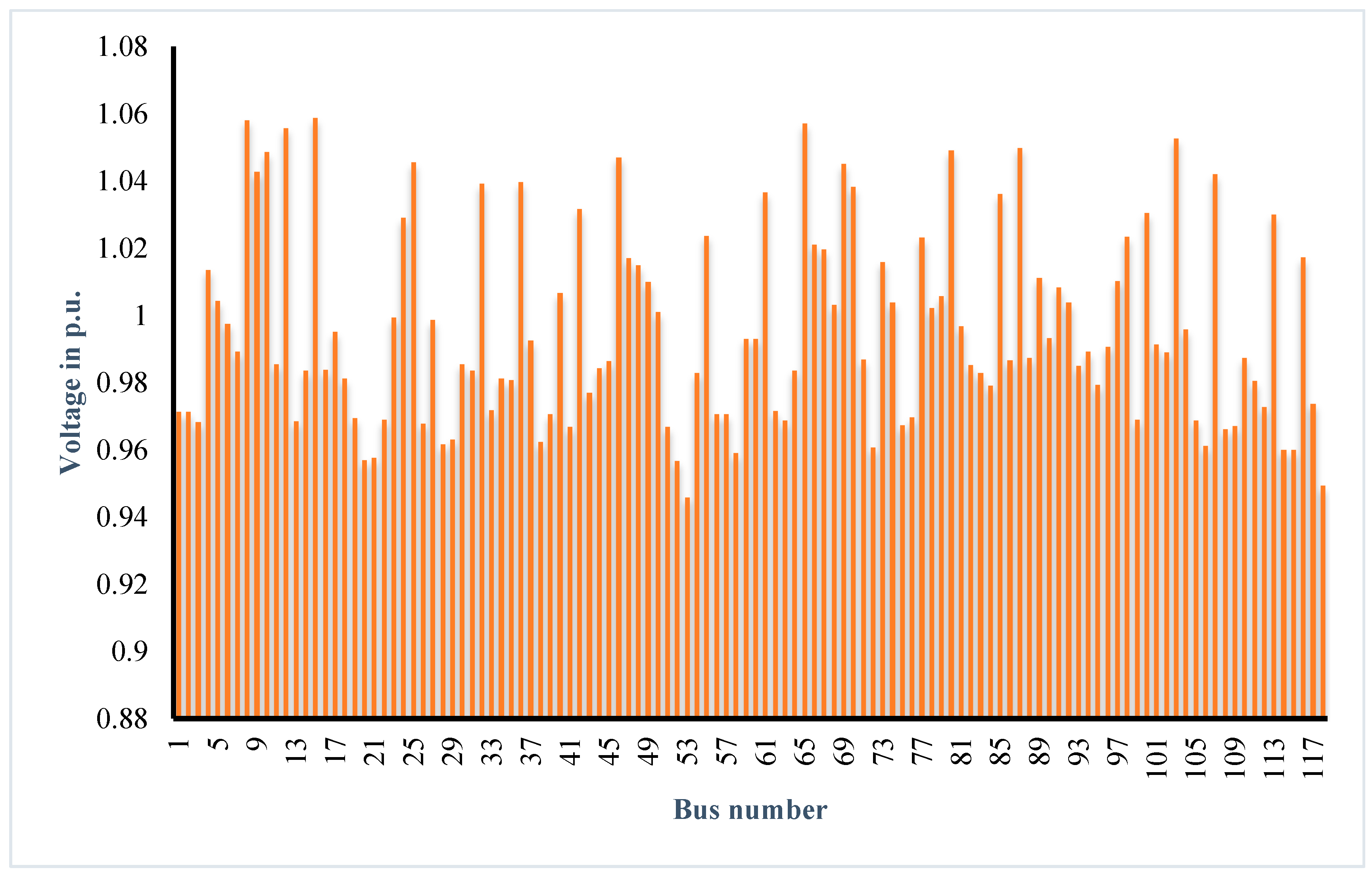
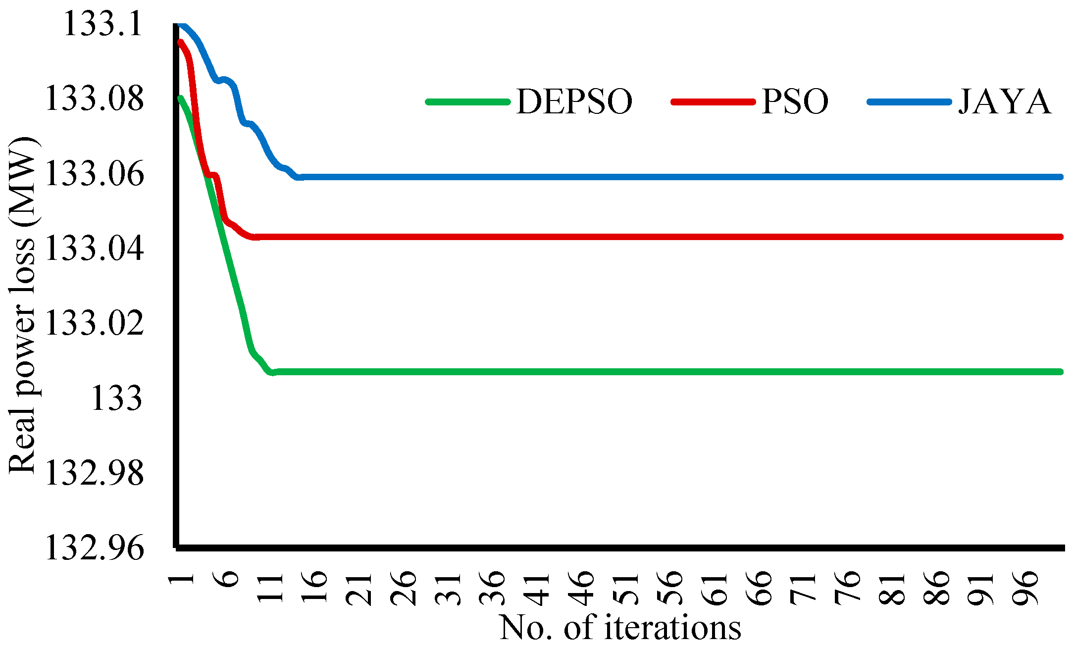
Figure 9 shows the voltage profile of all 118 buses in the test system. All bus voltages are found to be within the expected limits. The convergence plot of
Figure 10 shows that PSO converges first at the 9th iteration, DEPSO at the 11th iteration, and JAYA at the 14th iteration. Though PSO converges two iterations earlier, the objective function value obtained is greater than that for the DEPSO method. Hence, it is implicit that for providing an optimal or near-to-global optimal solution, the proposed method is comparatively better than the other methods.
6.4. Comparison with Existing Literature and Discussion
Most power system researchers have worked on the multi-objective RPD problem using swarm intelligence techniques that are either based on natural phenomena or physical phenomena [
30]. For establishing the potency of the proposed method, the results obtained for the IEEE 30-bus system has been compared to a handful of published results.
Comparison of results necessitates them to be worked out on the same platform with the same simulation conditions. The number of shunt devices in the IEEE 30-bus system has been increased for comparison purposes. Thus, the IEEE 30-bus system consists of six generators at buses 1, 2, 5, 8, 11, and 13, four tap-changing transformers at branches 6–9, 6–10, 4–12, and 27–28, and nine shunt compensators at 10, 12, 15, 17, 20, 21, 23, 24, and 29. The total load on the system is 283.4 MW. The base case current power loss is 5.833 MW.
Table 6 shows the values of power losses obtained using GSA [
31], OGSA [
32], ALC-PSO [
33], FAHCLPSO [
34], KHA [
35], and CKHA [
35]. GSA and OGSA stand for gravitational search algorithm and opposition-based GSA, respectively. Two modified forms of PSO—ALC-PSO, where ALC is ageing leader challenge and FAHCLPSO is the abbreviation for fuzzy adaptive heterogeneous comprehensive learning PSO. KHA is the acronym for krill herd algorithm and CKHA is chaotic KHA.
It is quite evident from
Table 6 that power loss is minimum for the case with optimal control variables calculated by the proposed DEPSO method. Losses obtained amount to 5.3474 MW, which is 8.3% less than the base case power loss.
6.5. Validation of the Method
Separate tests were conducted on the IEEE 118-bus system to corroborate the efficiency of the proposed DEPSO method considering three possible ways of handling the different types of variables. In the first method, all variables were considered to be continuous. Power losses were obtained to be 132.68 MW. The solution appears to be optimal but obviously not feasible. Secondly, values obtained for discrete variables were rounded off to the discrete steps nearest to their solution in the first case, and continuous variables were reiterated. The losses amounted to 133.043 MW. The solution will, of course, be feasible, but the losses are higher than the minimum value obtained in the previous method. As the third option, the DEPSO method was directly applied to obtain the control variable values. The peculiarity of the method is in maintaining the nature of variables throughout the search procedure, so that after each iteration, discrete variables will have only feasible discrete values. The losses obtained was 133.007 MW, which is less than those of the other two methods. The solution so obtained is feasible and optimal. The proposed method brings about a reduction in losses up to 3.6% more than the method of rounding.
7. Twenty-Four-Hour Scheduling
Reactive power dispatch can be done under the planning stage, as well as the scheduling stage. During the planning stage, procurement of possible reactive power sources, i.e., potential suppliers, is identified by the system operator at optimal locations. Once they are known, it is easy to allocate reactive power at the required time, during scheduling.
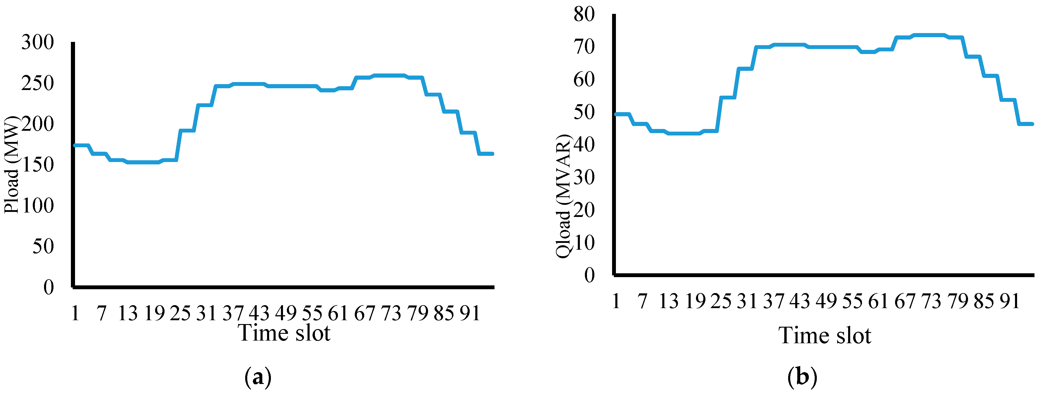
Figure 11a,b show typical real and reactive power load curves with respect to time, breaking up 24 h into 96 time slots, each of 15 min duration. Twenty-four-hour load data have been formulated from
Table 3 and
Table 4 of IEEE test bus data, available online based on the total load on the 14-bus IEEE test system.
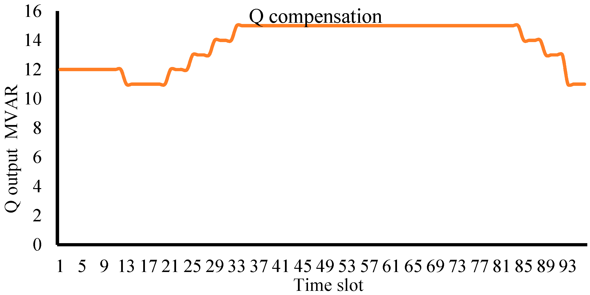
Based on the load variations in the system, optimal values for the control variables were calculated to meet the objective of real power loss minimization subject to constraints referred by (7)–(13) using the DEPSO method, for the whole 96 time slots. The output of the reactive power compensator (STATCOM) kept at bus 9 is shown in
Figure 12.
It has been observed that, up to 60% of the load on the system, the compensation needed to be provided is 11 MVAR. As the load increases, the compensation also increases, and when the load is more than 90%, the STATCOM under consideration should be made available operating at its full capacity of 15 MVAR. If the above information of load variation is known a priori, the operator will be able to adjust the control settings of compensation devices at appropriate time instants.
8. Conclusions
The aim of this research has been to investigate the usefulness of a novel technique, referred to as diversity-enhanced particle swarm optimization (DEPSO), for solving the multi-objective reactive power dispatch problem. In the DEPSO technique, all the variables preserve their nature from the start throughout the process of solving the problem. The method identifies divergence of the candidate solution from the best value and fetches back the particles that are deviating from the optimal solution. The preliminary investigations reveal the ability of the proposed method to search in large multi-dimensional solution space and determine the optimal solution containing integer, discrete, and continuous values. The methodology provides 8.3% less power losses than the base case losses when compared to results from existing literature. DEPSO provides 3.6% more power loss reduction than the conventional rounding-off method, thus making it more suitable than any other existing method to determine the feasible and optimal solution for the RPD problem. Further, the study on twenty-four-hour scheduling establishes the capability of the proposed method to be used in dynamic reactive power scheduling.
9. Future Scope
The conventional power grid is being subjected to drastic scheduled, as well as unscheduled, load changes under the present scenario. Effective reactive power forecasting and scheduling have become the need of the hour for maintaining system voltage stability. An optimal reactive power schedule, prepared based on estimated real and reactive power load data, on a real-time basis can benefit the system operator, preserving the grid stability. The proposed method of DEPSO is a promising approach for finding an optimal and feasible solution for the problem of the hour.
Author Contributions
Conceptualization, M.V. and S.K.T.K.; Methodology, M.V.; Software, M.V.; Validation, M.V. and S.K.T.K.; Formal Analysis, M.V.; Investigation, M.V.; Resources, M.V.; Data Curation, M.V. and S.K.T.K.; Writing-Original Draft Preparation, M.V.; Writing-Review & Editing, M.V. and S.K.T.K.; Supervision, S.K.T.K.; Project Administration, S.K.T.K. All authors have read and agreed to the published version of the manuscript.
Funding
This research received no external funding.
Conflicts of Interest
The authors declare no conflict of interest.
Appendix A
Voltages of the 54 generator buses in the IEEE 118-bus system for the three different formulations for the three algorithms are made available in
Table A1.
Table A1.
Optimal control variables (continuous only) for IEEE 118-bus using different algorithms.
Table A1.
Optimal control variables (continuous only) for IEEE 118-bus using different algorithms.
| Variable Name | Formulation I (P1 only) | Formulation II (P2 only) | Formulation III (P1 and P2) |
|---|
| PSO | DEPSO | JAYA | PSO | DEPSO | JAYA | PSO | DEPSO | JAYA |
|---|
| 1.04405 | 0.97126 | 1.01783 | 0.98472 | 1.00513 | 1.04486 | 1.07484 | 1.03733 | 0.99785 |
| 1.05163 | 1.0137 | 1.02283 | 1.01303 | 1.01923 | 0.98444 | 1.05537 | 1.05976 | 0.93687 |
| 1.05122 | 0.99767 | 1.0665 | 1.05746 | 1.03999 | 1.048 | 1.01643 | 1.04249 | 0.98172 |
| 1.07393 | 1.05832 | 1.05485 | 1.0389 | 1.04389 | 1.05462 | 1.01801 | 0.99763 | 0.98666 |
| 1.07011 | 1.04876 | 1.00435 | 1.02694 | 1.03365 | 1.03545 | 1.02326 | 1.00233 | 0.96511 |
| 1.05843 | 1.05595 | 1.00832 | 1.06118 | 0.98631 | 1.00227 | 1.03847 | 1.05746 | 1.07227 |
| 1.04603 | 1.05882 | 1.00132 | 1.02569 | 0.98626 | 1.01331 | 1.00053 | 1.00679 | 1.0166 |
| 1.03275 | 0.98123 | 0.93766 | 1.0037 | 1.03787 | 1.00994 | 0.99434 | 1.0454 | 1.01951 |
| 1.0535 | 0.96939 | 1.01 | 1.04825 | 1.04999 | 0.98069 | 1.06146 | 0.97817 | 1.02293 |
| 1.03518 | 1.02912 | 0.999126 | 1.0364 | 1.05489 | 0.95896 | 1.00606 | 1.0155 | 1.00471 |
| 1.04632 | 1.04562 | 1.00495 | 1.02882 | 1.02203 | 1.00923 | 1.02858 | 1.05485 | 1.03257 |
| 1.04945 | 0.96793 | 0.970941 | 1.05285 | 1.05759 | 0.97738 | 1.05308 | 0.99411 | 1.03525 |
| 1.03275 | 0.99872 | 1.00132 | 1.05453 | 1.03585 | 1.00325 | 1.06026 | 1.00036 | 0.98633 |
| 1.07357 | 0.9837 | 0.97001 | 1.07304 | 1.03916 | 0.95354 | 1.00773 | 0.96356 | 0.96796 |
| 1.0611 | 1.0393 | 1.01173 | 1.06069 | 0.97462 | 0.95311 | 1.06711 | 0.98246 | 0.97625 |
| 1.01604 | 0.98125 | 0.91600 | 1.01847 | 1.02059 | 1.01547 | 1.07162 | 1.01236 | 1.06989 |
| 1.03017 | 1.0398 | 1.05672 | 1.00627 | 1.03275 | 1.00295 | 1.01714 | 1.01169 | 1.01656 |
| 1.06466 | 1.00677 | 1.02954 | 1.02223 | 0.96984 | 1.01289 | 1.0602 | 1.03023 | 0.96831 |
| 0.97562 | 1.0318 | 0.95183 | 1.03361 | 1.00232 | 1.02707 | 0.99582 | 0.98826 | 0.95009 |
| 0.99267 | 1.0472 | 1.03486 | 1.05032 | 1.03702 | 1.02349 | 1.02997 | 1.05318 | 1.06984 |
| 0.99915 | 1.01001 | 1.09909 | 1.01698 | 1.0161 | 1.01403 | 1.01466 | 1.03625 | 0.98089 |
| 1.06713 | 0.98294 | 1.01958 | 1.04004 | 1.02187 | 0.96995 | 1.05459 | 1.03547 | 0.98806 |
| 1.03777 | 1.02385 | 0.97507 | 0.99865 | 0.95985 | 0.91244 | 1.03017 | 1.00546 | 1.12608 |
| 1.02999 | 0.97068 | 1.03283 | 1.012 | 1.03999 | 1.02143 | 1.01712 | 0.96231 | 1.08386 |
| 1.00749 | 0.99316 | 0.98893 | 1.04484 | 1.01693 | 0.96227 | 0.99566 | 1.00975 | 0.96318 |
| 0.98737 | 1.03674 | 1.06958 | 1.06339 | 0.98244 | 0.97389 | 0.98788 | 0.99035 | 0.93546 |
| 1.01004 | 0.97148 | 0.95074 | 1.06816 | 1.00468 | 0.97205 | 1.07048 | 0.99915 | 1.01476 |
| 0.9801 | 1.05733 | 0.98419 | 1.00202 | 1.0443 | 1.02547 | 1.04899 | 0.98172 | 1.00472 |
| 0.99795 | 1.02123 | 1.01505 | 1.03369 | 1.031 | 1.03336 | 1.01939 | 0.96631 | 0.99077 |
| 0.97684 | 1.04517 | 1.06541 | 1.00819 | 0.97120 | 0.97987 | 1.00209 | 1.03681 | 1.03205 |
| 0.98654 | 1.03831 | 0.99533 | 1.03859 | 0.98660 | 1.01812 | 1.03156 | 0.97484 | 1.00787 |
| 1.05564 | 0.96082 | 0.99910 | 1.06162 | 1.00245 | 0.97072 | 1.00725 | 0.98658 | 0.96049 |
| 1.01217 | 1.01605 | 1.01581 | 0.99188 | 0.96749 | 1.04067 | 1.07475 | 1.00336 | 0.93846 |
| 1.07012 | 1.00392 | 1.06197 | 1.02003 | 1.04743 | 1.00113 | 1.06178 | 0.98937 | 1.01323 |
| 0.99195 | 0.96965 | 0.98696 | 0.99641 | 1.00314 | 0.98223 | 1.02159 | 1.03771 | 1.00466 |
| 0.99093 | 1.02329 | 0.97971 | 1.01821 | 1.05106 | 1.02982 | 1.07215 | 0.97280 | 1.04341 |
| 1.03306 | 1.0493 | 0.93322 | 1.05558 | 0.96902 | 0.98781 | 1.06523 | 1.01941 | 0.89990 |
| 1.02528 | 1.03626 | 0.79979 | 1.0638 | 0.98044 | 0.99330 | 1.02026 | 0.99738 | 1.03873 |
| 1.06623 | 1.05006 | 1.02951 | 1.00312 | 1.02035 | 0.98506 | 0.98686 | 1.02744 | 1.00327 |
| 1.02528 | 1.01124 | 1.04421 | 1.03 | 0.99781 | 0.89705 | 0.99318 | 1.0076 | 1.01634 |
| 0.97508 | 0.99337 | 1.02412 | 0.98521 | 0.99955 | 0.96645 | 0.99308 | 0.96879 | 0.95638 |
| 1.03314 | 1.00832 | 1.11079 | 0.99132 | 0.99223 | 0.96558 | 1.00457 | 0.96209 | 1.05205 |
| 1.06474 | 1.00394 | 0.95488 | 0.97865 | 1.04997 | 0.98539 | 1.02377 | 1.01388 | 1.01833 |
| 1.07394 | 0.96889 | 0.93078 | 0.99901 | 1.04385 | 1.01607 | 1.06574 | 0.96941 | 0.99338 |
| 1.01721 | 1.0306 | 0.96774 | 0.99914 | 0.96243 | 1.03615 | 1.04902 | 1.03927 | 1.04968 |
| 1.04544 | 1.05279 | 1.03539 | 1.03806 | 0.99511 | 0.99668 | 0.97955 | 1.04313 | 0.99900 |
| 1.06821 | 0.99595 | 1.04051 | 1.00435 | 1.04093 | 0.97182 | 0.97748 | 1.04483 | 0.97507 |
| 1.02544 | 0.96885 | 1.06427 | 1.06332 | 0.99018 | 0.96457 | 1.0092 | 0.98834 | 0.97365 |
| 1.04886 | 1.04219 | 1.11941 | 0.99475 | 0.99955 | 1.03267 | 1.05392 | 0.97963 | 1.02122 |
| 0.9892 | 0.98739 | 1.02914 | 1.00869 | 0.96797 | 0.94179 | 1.04299 | 1.05416 | 1.07737 |
| 0.99526 | 0.98059 | 0.98405 | 1.04246 | 1.02685 | 0.992053 | 1.05757 | 0.97536 | 0.96411 |
| 1.0568 | 0.97289 | 1.10282 | 1.04399 | 0.96831 | 0.99397 | 1.05514 | 0.97039 | 1.03667 |
| 0.98476 | 1.03008 | 0.97432 | 0.99553 | 0.96246 | 0.99611 | 1.00281 | 0.98859 | 1.00727 |
| 0.99674 | 1.01739 | 1.11129 | 1.01059 | 1.02358 | 1.07122 | 0.98224 | 0.96757 | 0.95373 |
References
- Dommel, H.W.; Tinney, W.F. Optimal Power flow solutions. IEEE Trans. PAS 1968, 87, 1866–1876. [Google Scholar] [CrossRef]
- Iyer, S.R.; Ramachandran, K.; Hariharan, S. Optimal reactive power allocation for improved system performance. IEEE Trans. PAS 1984, 103, 1509–1515. [Google Scholar] [CrossRef]
- Mansour, M.O.; Rehman, T.M.A. Non-linear VAR Optimization using Decomposition and Coordination. IEEE Trans. PAS 1984, 103, 246–255. [Google Scholar] [CrossRef]
- Granville, S. An Interior Point Method based Optimal Power Flow. IEEE Trans. Power Syst. 1994, 9, 136–146. [Google Scholar] [CrossRef]
- Wei, H.; Sasaki, H.; Kubokawa, J.; Yokohama, R. An interior point nonlinear programming for optimal power flow problems with a new data structure. IEEE Trans. Power Syst. 1998, 12, 444–877. [Google Scholar]
- Momoh, J.A.; Koesslar, R.J.; Bond, M.S.; Stott, B.; Sun, D.; Papalexopoulos, A.; Ristanovic, P. Challenges to optimal power flow. IEEE Trans. Power Syst. 1997, 12, 444–455. [Google Scholar] [CrossRef]
- Tinney, W.F.; Bright, J.; Damaree, K.; Hughes, B. Some deficiencies in optimal power flows. IEEE Trans. Power Syst. 1987, 3, 164–169. [Google Scholar] [CrossRef]
- Wu, Q.H.; Ma, J.T. Power System Optimal Reactive Power Dispatch using Evolutionary Programming. IEEE Trans. Power Syst. 1995, 10, 1243–1249. [Google Scholar] [CrossRef]
- Lai, L.L.; Ma, J.T. Application of Evolutionary Programming to Reactive Power Planning—Comparison with non-linear programming approach. IEEE/PES Winter Meet. 1996, 96, 248–255. [Google Scholar]
- Abido, M.A. Multiobjective Optimal VAR Dispatch using Strength Pareto Evolutionary Algorithm. In Proceedings of the 2006 IEEE International Conference on Evolutionary Computation, Vancouver, BC, Canada, 16–21 July 2006; pp. 730–736. [Google Scholar]
- Vaisakh, K.; Rao, P.K. Comparison and Application of Self-Tuning DE/HDE based Algorithms to solve Optimal Reactive Power Dispatch Problems with Multiple Objectives. In Proceedings of the IEEE World Congress on Nature & Biologically Inspired Computing (NaBIC 2009), Coimbatore, India, 9–11 December 2009; pp. 1168–1173. [Google Scholar]
- Devaraj, D.; Rosylin, J.P. Genetic Algorithm based Reactive Power Dispatch for Voltage Stability improvement. Int. J. Electr. Power Energy Syst. 2010, 32, 1151–1156. [Google Scholar] [CrossRef]
- Esmin Ahmed, A.A.; Torres, G.L.; Cao, Y.J. Application of Particle Swarm Optimization to Optimal Power Systems. Int. J. Innov. Comput. Inf. Control 2012, 8, 1705–1716. [Google Scholar]
- Varadarajan, M.; Swarup, K.S. Differential Evolutionary Algorithm for Optimal Reactive Power Dispatch. Int. J. Electr. Power Energy Syst. 2008, 30, 435–441. [Google Scholar] [CrossRef]
- Sujin, P.R.; Prakash, T.R.D.; Linda, M.M. Particle Swarm Optimization Based Reactive Power Optimization. J. Comput. 2010, 2, 73–78. [Google Scholar]
- Khanmiri, D.T.; Nasiri, N.; Abedinzadeh, T. Optimal Reactive Power Dispatch using an Improved Genetic Algorithm. Int. J. Comput. Electr. Eng. 2012, 4, 463–466. [Google Scholar]
- Soler, E.M.; Asada, E.N.; da Costa, G.R.M. Penalty based Non-linear Solver for Optimal Reactive Power Dispatch with Discrete Controls. IEEE Trans. Power Syst. 2013, 28, 2174–2182. [Google Scholar] [CrossRef]
- Mouassa, S.; Bouktir, T.; Salhi, A. Ant-lion Optimizer for solving Optimal Reactive Power Dispatch problem in power systems. Int. J. Eng. Sci. Technol. 2017, 20, 885–895. [Google Scholar] [CrossRef]
- Palappan, A.; Thangavelu, J. A new meta-heuristic Dragon-fly optimization algorithm for Optimal Reactive Power Dispatch Problem. Gazi Univ. J. Sci. 2018, 31, 1107–1121. [Google Scholar]
- Sahli, Z.; Hamouda, A.; Bekrar, A.; Trentesaux, D. Reactive Power Dispatch Optimization with Voltage Profile Improvement using an Efficient Hybrid Algorithm. Energies 2018, 11, 2134. [Google Scholar] [CrossRef]
- Aljohani, T.M.; Ebrahim, A.F.; Mohammed, O. Single and Multiobjective Optimal Reactive Power Dispatch based on Hybrid Artificial Physics—Particle Swarm Optimization. Energies 2019, 12, 2333. [Google Scholar] [CrossRef]
- Packiasudha, M.; Suja, S.; Jerome, J. A new Cumulative Gravitational Search algorithm for optimal allocation of FACT device to minimize system loss in deregulated electrical power environment. Int. J. Electr. Power Energy Syst. 2017, 84, 34–46. [Google Scholar] [CrossRef]
- Eberhart, R.; Kennedy, J. Particle Swarm Optimization. In Proceedings of the ICNN’95–International Conference on Neural Networks, Perth, Australia, 27 November–1 December 1995; Volume IV, pp. 1942–1948. [Google Scholar]
- Riget, J.; Vesterstorm, J. A Diversity Guided Particle Swarm Optimizer—The ARPSO; Technical Report; (riget: 2002: DGPSO), no. 2 EVA Life; Department of Computer Science, University of Aarhus: Aarhus, Denmark, 2002. [Google Scholar]
- Deb, K.; Goyal, M. Optimizing engineering designs using a combined genetic search. In Proceedings of the 7th International Conference on Genetic Algorithm, East Lansing, MI, USA, 19–23 July 1997; pp. 512–527. [Google Scholar]
- Nakisa, B.; Rastgoo, M.N. A Survey: Particle Swarm Optimization based Algorithms to solve Premature Convergence Problem. J. Comput. Sci. 2014, 10, 1758–1765. [Google Scholar] [CrossRef]
- Pant, M.; Radha, T.; Singh, V.P. A Simple Diversity Guided Particle Swarm Optimization. In Proceedings of the 2007 IEEE Congress on Evolutionary Computation, Singapore, 25–28 September 2007; pp. 3294–3299. [Google Scholar]
- Rao, R.V. Jaya: A simple and new optimization algorithm for solving constrained and un-constrained optimization problems. Int. J. Ind. Eng. Comput. 2016, 7, 19–34. [Google Scholar]
- Power System Test Case Archive-UWEE. Available online: http://www.ee.washington.edu/research/pstca/ (accessed on 2 June 2019).
- Saddique, M.S.; Bhatti, A.R.; Haroon, S.S.; Sattar, M.K.; Amin, S.; Sajjad, A.I.; ul Haq, S.S.; Awan, A.B.; Rasheed, N. Solution to optimal reactive power dispatch in transmission system using meta-heuristic techniques—Status and technological review. Electr. Power Syst. Res. 2020, 178, 106031. [Google Scholar] [CrossRef]
- Duman, S.; Sonmez, Y.; Güvenç, U.; Yörükeren, N. Optimal reactive power dispatch using a gravitational search algorithm. IET Gener. Transm. Distrib. 2012, 6, 563–576. [Google Scholar] [CrossRef]
- Shaw, B.; Mukherjee, V.; Ghoshal, S.P. Solution of reactive power dispatch of power systems by an opposition-based gravitational search algorithm. Int. J. Electr. Power Energy Syst. 2014, 55, 29–40. [Google Scholar] [CrossRef]
- Singh, R.P.; Mukherjee, V.; Ghoshal, S.P. Optimal reactive power dispatch by particle swarm optimization with an aging leader and challengers. Appl. Soft Comput. 2015, 29, 298–309. [Google Scholar] [CrossRef]
- Naderi, E.; Narimani, H.; Fathi, M.; Narimani, M.R. A novel fuzzy adaptive configuration of particle swarm optimization to solve large-scale optimal reactive power dispatch. Appl. Soft Comput. 2017, 53, 441–456. [Google Scholar] [CrossRef]
- Mukherjee, A.; Mukherjee, V. Solution of optimal reactive power dispatch by chaotic krill herd algorithm. Trans. Distrib. IET Gener. 2015, 9, 2351–2362. [Google Scholar] [CrossRef]
© 2020 by the authors. Licensee MDPI, Basel, Switzerland. This article is an open access article distributed under the terms and conditions of the Creative Commons Attribution (CC BY) license (http://creativecommons.org/licenses/by/4.0/).


