Control of Heat Pumps with CO2 Emission Intensity Forecasts

 , , , and
Abstract
1. Introduction
2. Data
3. Model
3.1. Assumptions
3.2. State Space Equations
3.3. MPC
4. Inputs for the Model
Forecasts
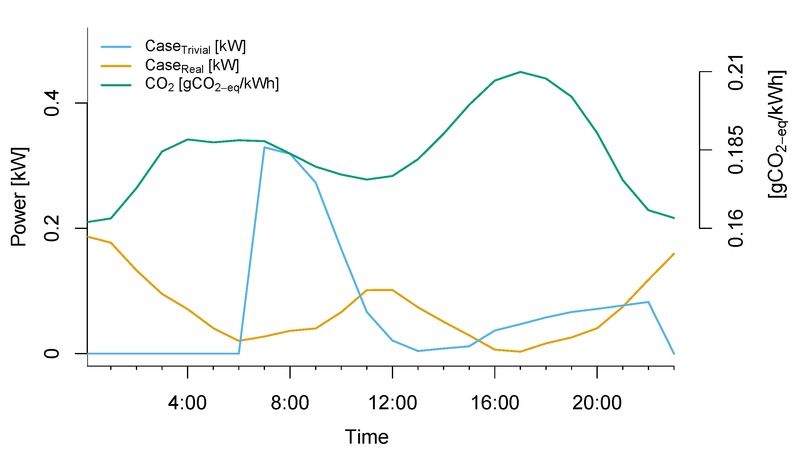
- CaseIdeal: This takes the exact value of a future CO emission intensity as prediction hence, a perfect forecast. This provides an upper limit of CO savings.
- CaseReal: This takes the CO emission forecast developed in Reference [18] and represents the performance of the MPC with real forecasts.
- CaseTrivial: This makes no use of forecasts and will thus result in a non predictive controller that simply controls the heat pump keeping the temperature at the lower limit if possible.
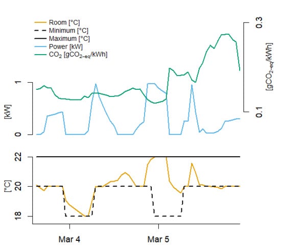
5. Results and Discussion
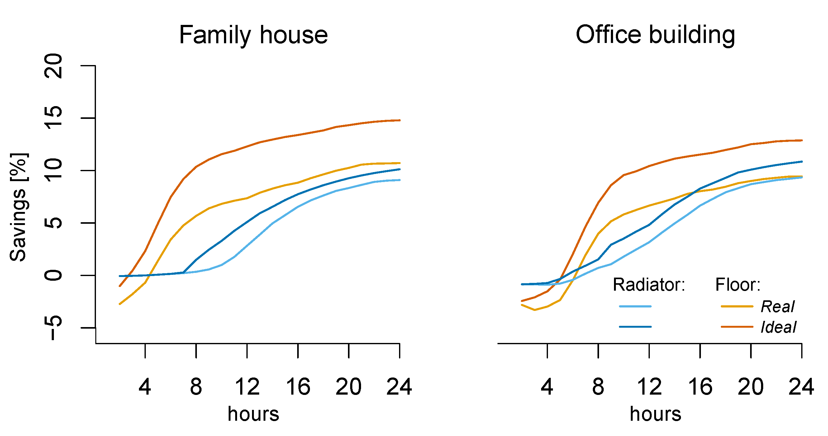
- Heating system and varying set points: Both radiator and floor heating are considered and the use of varying set points (lower temperature during the night).
- Horizon of forecasts: To get an idea about how long horizons actually are needed to get a well performing MPC.
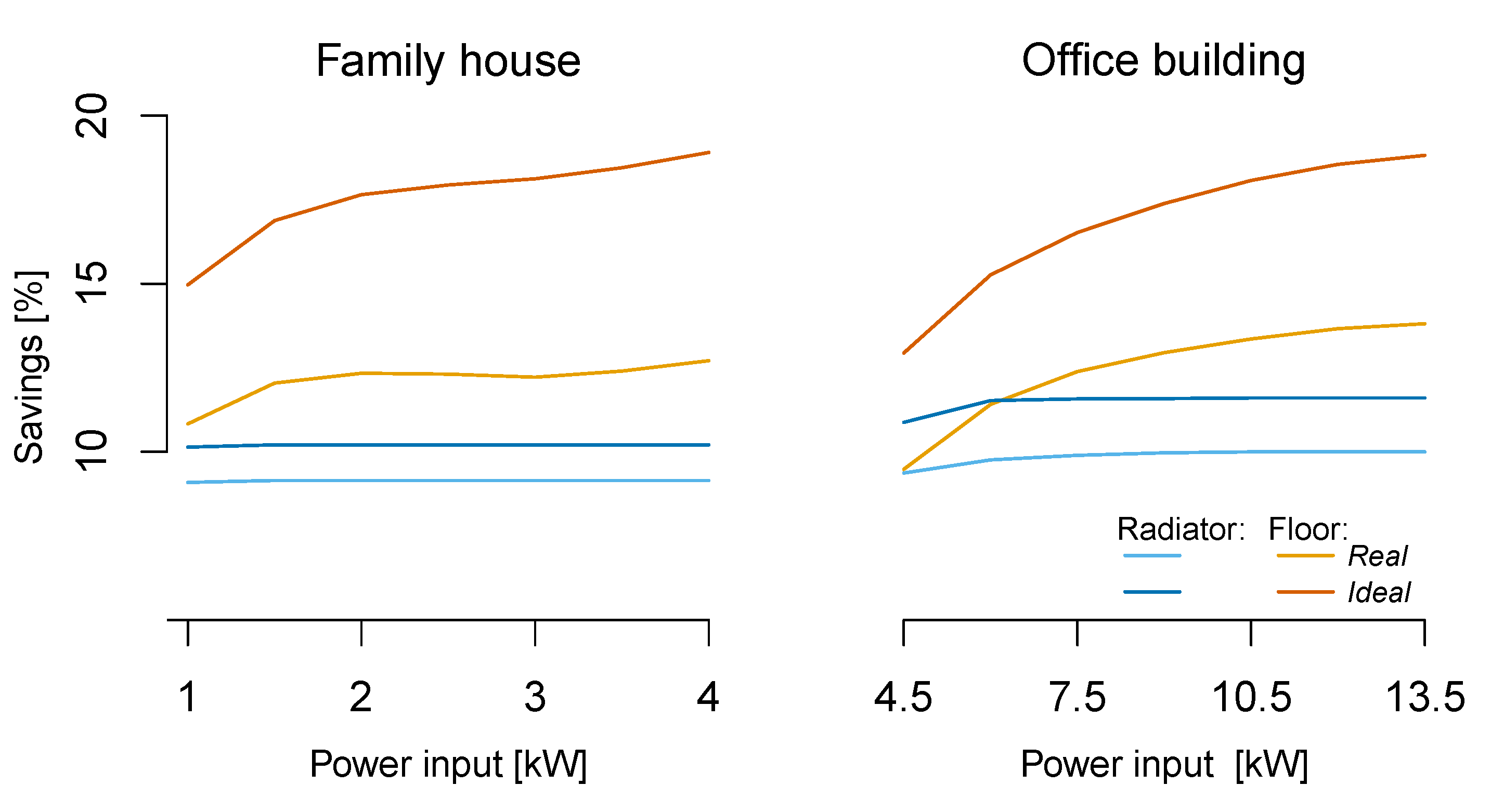
- Size of heat pumps: Essential for comparing the buildings and to know whether the potential is reached. Also economically, this is important because as the price increases with larger heat pumps. This will become a compromise between price and CO emission. The default values for the family house and office are the minimum sizes required to meet the heat demand on the coldest day (−12 C); 3 and 13 kWheat respectively Appendix (see Appendix C for calculations). Requirements are thus a 1 and 4.3 kW input signal respectively according to Equation (1).
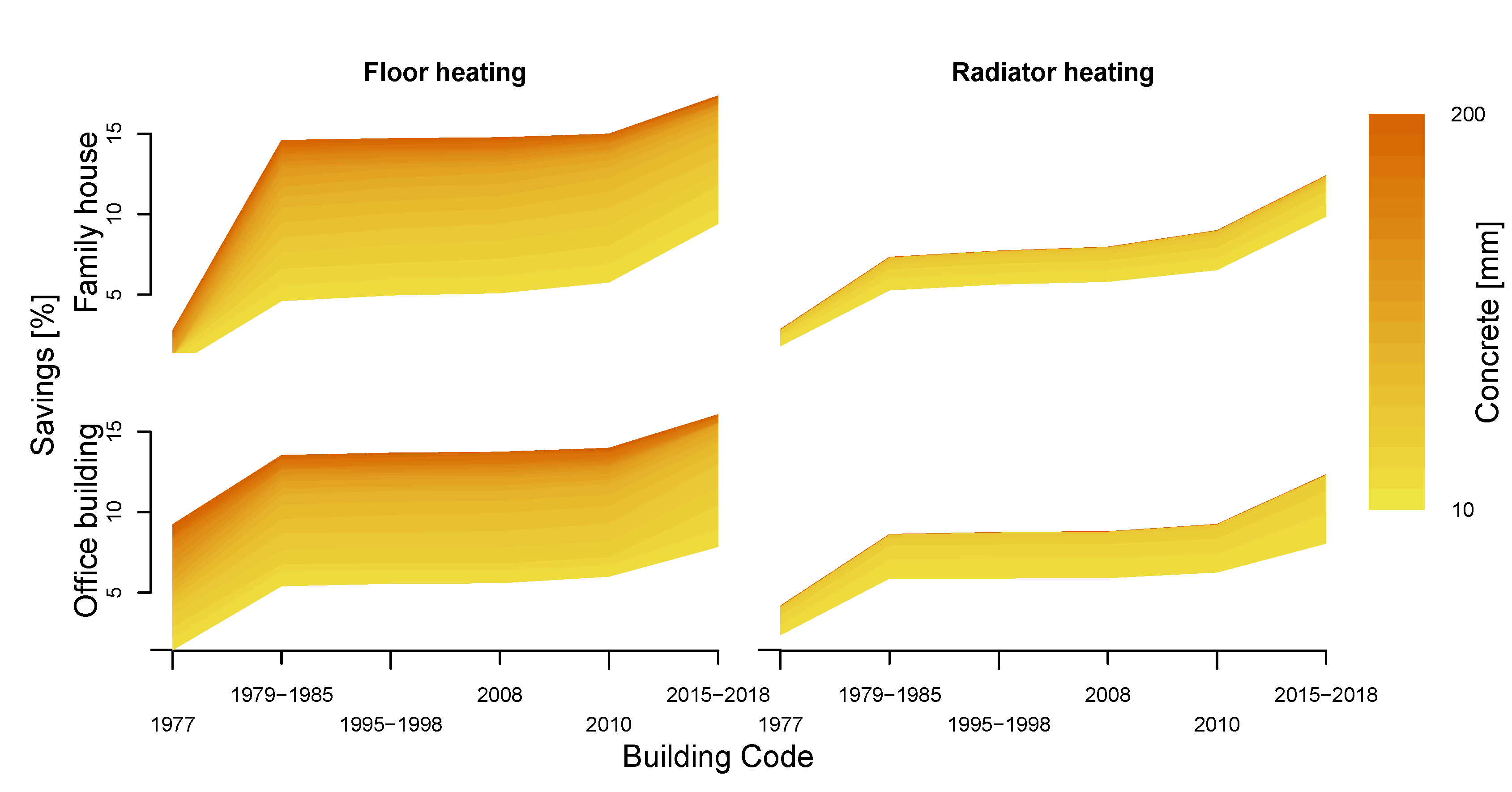
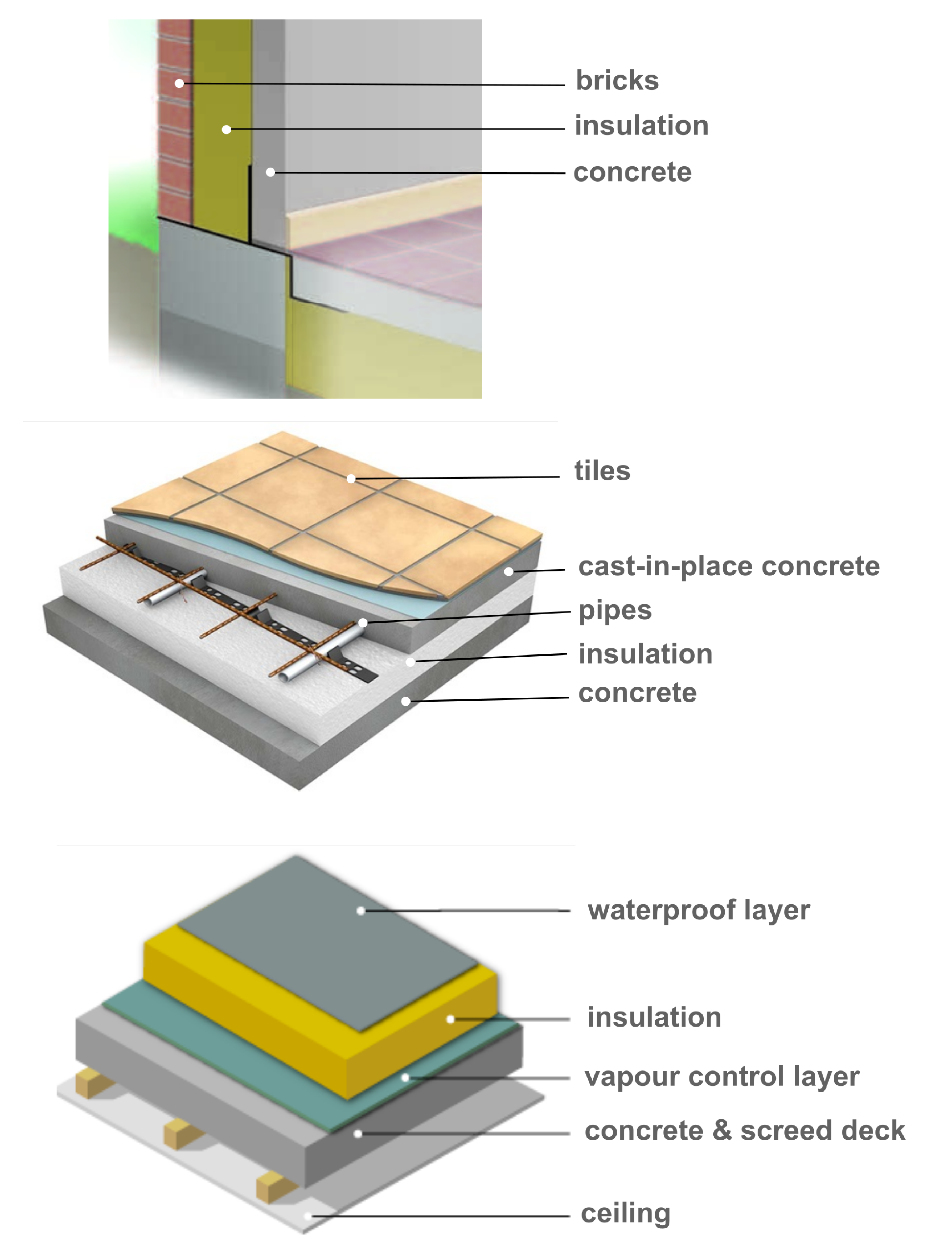
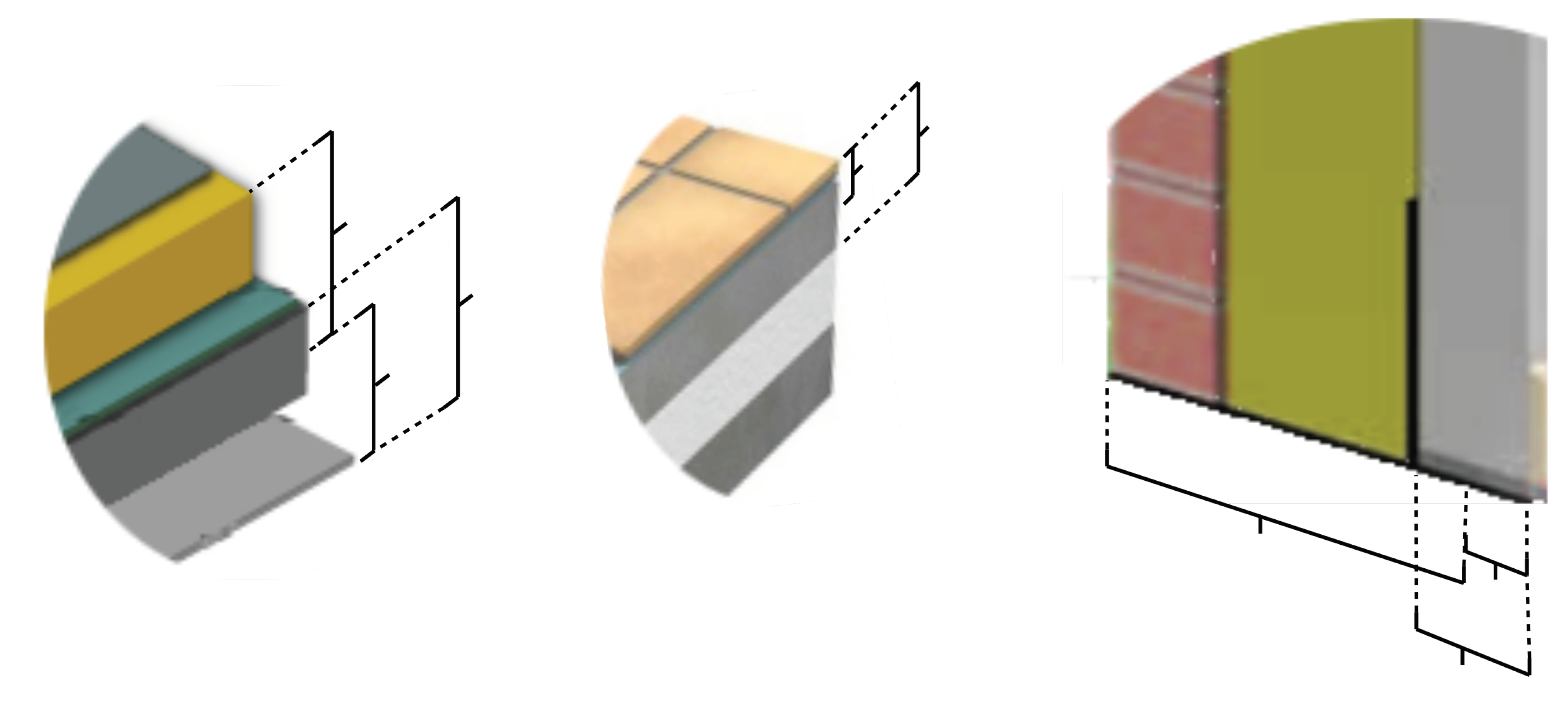
- Insulation and concrete thicknesses: These will be adjusted to see the impact of levels of insulation and heat capacity. The default thicknesses and material properties are shown in Appendix C.
Model Simplification
6. Conclusions
Author Contributions
Funding
Acknowledgments
Conflicts of Interest
Abbreviations
| MDPI | Multidisciplinary Digital Publishing Institute |
| CHP | Combined Heat and Power |
| MPC | Model Predictive Control |
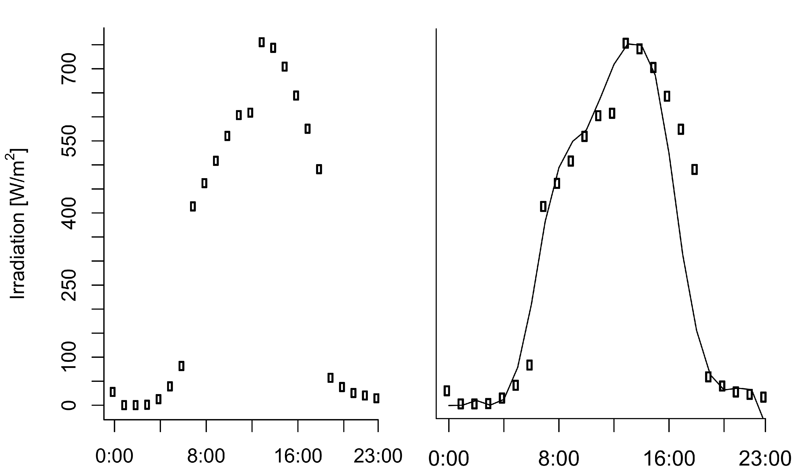
Appendix A. Kernel Smoothing

Appendix B. Building Parts


Appendix C. Parameter Estimation and Heat Pump Dimensions

 |
Heat Pump Dimensions
References
- Status of Power System Transformation 2019: Power System Flexibility. 2019. In International Energy Agency. Available online: https://www.iea.org (accessed on 6 November 2019).
- Huber, M.; Dimkova, D.; Hamacher, T. Integration of wind and solar power in Europe: Assessment of flexibility requirements. Energy 2003, 69, 236–246. [Google Scholar] [CrossRef]
- Lund, H.; Mathiesen, B.V. Characterizing the energy flexibility of buildings and districts. Appl. Energy 2018, 225, 175–182. [Google Scholar] [CrossRef]
- Bygninger og deres opvarmede areal efter område, tid, opvarmingsform, anvendelse, opførelsesår og enhed. 2019. By Danmarks Statistik. Available online: https://www.statistikbanken.dk/BOL102 (accessed on 27 November 2019).
- Danish Building Regulations 2018 (BR18); Ministry of Transport, Building and Housing: Copenhagen, Denmark, 2018.
- Halvgaard, R.; Kjølstad Poulsen, N.; Madsen, H.; Bagterp Jørgensen, J. Economic Model Predictive Control for Building Climate Control in a Smart Grid. In Proceedings of the 2012 IEEE PES Innovative Smart Grid Technologies (ISGT), Copenhagen, Denmark, 6–9 Ocotber 2012. [Google Scholar] [CrossRef]
- Corradi, O.; Ochsenfeld, H.; Madsen, H.; Pinson, P. Controlling Electricity Consumption by Forecasting its Response to Varying Prices. IEEE Trans. Power Syst. 2013, 28. [Google Scholar] [CrossRef]
- Clauß, J.; Stinner, S.; Solli, C.; Lindberg, K.B.; Madsen, H.; Georges, L. Evaluation Method for the Hourly Average CO2eq. Intensity of the Electricity Mix and Its Application to the Demand Response of Residential Heating. Energies 2019, 12, 1345. [Google Scholar] [CrossRef]
- Oldewurtel, F.; Parisio, A.; Jones, C.N.; Gyalistras, D.; Gwerder, M.; Stauch, V.; Lehmann, B.; Morari, M.; Berkelaar, M.; Eikland, K.; et al. Use of model predictive control and weather forecasts for energy efficient building climate control. Energy Build. 2012, 45, 15–17. [Google Scholar] [CrossRef]
- Oldewurtel, F.; Sturzenegger, D.; Morari, M. Importance of occupancy information for building climate control. Appl. Energy 2013, 101, 521–532. [Google Scholar] [CrossRef]
- Killian, M.; Mayer, B.; Kozek, M. Cooperative fuzzy model predictive control for heating and cooling of buildings. Energy Build. 2016, 112, 130–140. [Google Scholar] [CrossRef]
- Lindelöf, D.; Afshari, H.; Alisafaee, M.; Biswas, J.; Caban, M.; Mocellin, X.; Viaene, J. Field tests of an adaptive, model-predictive heating controller for residential buildings. Energy Build. 2016, 99, 292–302. [Google Scholar] [CrossRef]
- Chen, C.; Wang, J.; Heo, Y.; Kishore, S. MPC-based appliance scheduling for residential building energy management controller. IEEE Trans. Smart Grid 2016, 4, 1401–1410. [Google Scholar] [CrossRef]
- Chen, C.; Wang, J.; Heo, Y.; Kishore, S. Ten questions concerning model predictive control for energy efficient buildings. Energy Build. 2016, 105, 403–412. [Google Scholar] [CrossRef]
- Hammerstrom, D. Pacific Northwest GridWise™ Testbed Demonstration Projects. Part I; Pacific Northwest National Lab: Richland, WA, USA, 2007.
- Wagner, U.; Mauch, W.; von Roon, S. Das Merit-Order-Dilemma der Emissionen; Forschungsstelle für Energiewirtschaft e.V.: Munich, Germany, 2002. [Google Scholar]
- Regettt, A.; Böing, F.; Conrad, J.; Fattler, S.; Kranner, C. Emission Assessment of Electricity: Mix vs. Marginal Power Plant Method. In Proceedings of the 15th International Conference on the European Energy Market (EEM), Lodz, Poland, 27–29 June 2018. [Google Scholar] [CrossRef]
- Leerbeck, K.; Bacher, P.; Junker, R.; Goranović, G.; Corradi, O.; Ebrahimy, R.; Tveit, A.; Madsen, H. Short-Term Forecasting of CO2 Emission Intensity in Power Grids by Machine Learning. arXiv, 2020; arXiv:2003.05740. [Google Scholar]
- Corradi, O. Estimating the marginal carbon intensity of electricity with machine learning. 2018. in Medium. Available online: https://medium.com/ (accessed on 1 November 2019).
- Bialek, J. Tracing the flow of electricity. Iee Proc. Gener. Transm. Distrib. 1996, 143, 313–320. [Google Scholar] [CrossRef]
- Bialek, J. Contributions of Individual Generators to Loads and Flows. Trans. Power Syst. 1997, 12, 52–60. [Google Scholar] [CrossRef]
- Verhlst, C.; Logist, F.; Van Impe, J.; Helsen, L. Study of the optimal control problem formulation for modulating air-to-water heat pumps connected to a residential floor heating system. Energy Build. 2011, 45, 43–53. [Google Scholar] [CrossRef]
- Hangos, K.M.; Bokor, J.; Szederkényi, G. Analysis and Control of Nonlinear Process Systems; Springer: Berlin, Germany, 2003; pp. 39–71. [Google Scholar]
- Madsen, H.; Holst, J. Estimation of continuous-time models for the heat dynamics of a building. Energy Build. 1995, 22, 67–79. [Google Scholar] [CrossRef]
- Madsen, H. Time Series Analysis; Chapman & Hall/CRC—Taylor & Francis Group: Boca Raton, FL, USA, 2007. [Google Scholar]
- Bacher, P.; Madsen, H. Identifying suitable models for the heat dynamics of buildings. Energy Build. 2011, 43, 1511–1522. [Google Scholar] [CrossRef]
- Cengel, Y.; Boles, M.A. Thermodynamics—An Engineering Approach; McGraw Hill: New York, NY, USA, 2010; pp. 82–84. [Google Scholar]
- Coefficient of Performance. 2019. For De Kleijn Energy Consultants & Engineers. Available online: http://industrialheatpumps.nl/en/how_it_works/cop_heat_pump/ (accessed on 16 December 2019).
- Berkelaar, M.; Eikland, K.; Notebaert, P. lpsolve: Open Source (Mixed-Integer) Linear Programming System. 2004. Available online: http://lpsolve.sourceforge.net/5.5/ (accessed on 2 May 2020).
- Den Lille Lune. ROCKWOOL A/S. 2018. 34p. Available online: https://www.rockwool.dk/siteassets/o2-rockwool/dokumentation-og-certifikater/brochurer/bygningsisolering/den-lille-lune-rockwool.pdf (accessed on 2 May 2020).
- Viden Om Vinduer. 2020. By Energi Styrelsen. Available online: http://www.vinduesvidensystem.dk/ruder.html (accessed on 8 January 2020).
- Grønborg, R.; Armin, A.; Lopes, G.; Amaral, R.; Lindberg, K.B.; Reynders, G.; Relan, R.; Madsen, H. Characterizing the energy flexibility of buildings and districts. Appl. Energy 2018, 225, 175–182. [Google Scholar] [CrossRef]
- Brøgger, M.; Bacher, P.; Madsen, H.; Wittchen, K.B. Estimating the influence of rebound effects on the energy-saving potential in building stocks. Energy Build. 2018, 181, 62–74. [Google Scholar] [CrossRef]
- 50% Wind Power in Denmark in 2025; Ea Energy Analyses: Copenhagen, Denmark, 2007.
- Lund, H.; Mathiesen, B.V. Energy system analysis of 100% renewable energy systems—The case of Denmark in years 2030 and 2050. Energy 2009, 34, 524–531. [Google Scholar] [CrossRef]
- Hastie, T.; Tibshirani, R.; Friedman, J. The Elements of Statistical Learning; Springer Series in Statistics; Springer: Berlin, Germany, 2017; pp. 141–146. [Google Scholar]
- Fix—rør i Monteringsbånd til Indstøbning. 2019. By Uponor. Available online: https://www.uponor.dk/vvs/produkter/gulvvarme/fix-gulvvarme-i-monteringsband (accessed on 1 November 2019).
- Housing Retrofit: Concrete Flat Roof Insulation. 2019. By Greenspec. Available online: http://www.greenspec.co.uk/building-design/concrete-flat-roof-insulation/ (accessed on 1 November 2019).
- French Building Energy and Thermal Regulation; CSTB FR: Marne-la-Vallee, France, 2005.


| BC | Walls | Roof | Doors | Windows | ||
|---|---|---|---|---|---|---|
| Year | ||||||
| 1977 | 1 | 0.45 | 3.6 | 3.6 | −174.314 ** | 0.777 ** |
| 1979–1985 | 0.4 | 0.2 | 2 | 2.9 | −117.378 ** | 0.744 ** |
| 1995–1998 | 0.4 | 0.2 | 2 | 2.3 | −69.934 ** | 0.709 ** |
| 2008 | 0.4 | 0.2 | 2 | 2 | −46.909 ** | 0.688 ** |
| 2010 | 0.3 | 0.2 | 2 | 1.8 ** | −33 | 0.673 ** |
| 2015–2018 | 0.14 * | 0.1 * | 2 | 1.6 ** | −17 | 0.654 ** |
| Family House | Office Building | ||
|---|---|---|---|
| 156 | 1250 | ||
| 107 | 302 | ||
| 4 | 13 | ||
| 14 | 39 | ||
| 10.398 | 2.379 | ||
| 1.190 | 0.269 | ||
| 1.442 | 0.180 | ||
| 7.508 | 39.527 | ||
| 3.198 | 25.623 | ||
| 0.876 | 6.944 |
| Floor | Radiator | |||
|---|---|---|---|---|
| BC | BC | BC | BC | |
| Family house | ||||
| Min. savings | 0.5% | 9.4% | 1.8% | 9.9% |
| Max. savings | 2.7% | 17.4% | 2.8% | 12.4% |
| Office building | ||||
| Min. savings | 1.4% | 7.8% | 2.4% | 8.1% |
| Max. savings | 9.2% | 16.0% | 4.1% | 12.3% |
© 2020 by the authors. Licensee MDPI, Basel, Switzerland. This article is an open access article distributed under the terms and conditions of the Creative Commons Attribution (CC BY) license (http://creativecommons.org/licenses/by/4.0/).
Share and Cite
Leerbeck, K.; Bacher, P.; Junker, R.G.; Tveit, A.; Corradi, O.; Madsen, H.; Ebrahimy, R. Control of Heat Pumps with CO2 Emission Intensity Forecasts. Energies 2020, 13, 2851. https://doi.org/10.3390/en13112851
Leerbeck K, Bacher P, Junker RG, Tveit A, Corradi O, Madsen H, Ebrahimy R. Control of Heat Pumps with CO2 Emission Intensity Forecasts. Energies. 2020; 13(11):2851. https://doi.org/10.3390/en13112851
Chicago/Turabian StyleLeerbeck, Kenneth, Peder Bacher, Rune Grønborg Junker, Anna Tveit, Olivier Corradi, Henrik Madsen, and Razgar Ebrahimy. 2020. "Control of Heat Pumps with CO2 Emission Intensity Forecasts" Energies 13, no. 11: 2851. https://doi.org/10.3390/en13112851
APA StyleLeerbeck, K., Bacher, P., Junker, R. G., Tveit, A., Corradi, O., Madsen, H., & Ebrahimy, R. (2020). Control of Heat Pumps with CO2 Emission Intensity Forecasts. Energies, 13(11), 2851. https://doi.org/10.3390/en13112851