Article

Multi-Objective Optimization of Home Appliances and Electric Vehicle Considering Customer’s Benefits and Offsite Shared Photovoltaic Curtailment

School of Integrated Technology, Gwangju Institute of Science and Technology, 123 Cheomdangwagi-ro, Buk-gu, Gwangju 61005, Korea
*
Author to whom correspondence should be addressed.
Energies 2020, 13(11), 2852; https://doi.org/10.3390/en13112852
Submission received: 6 May 2020 / Revised: 28 May 2020 / Accepted: 30 May 2020 / Published: 3 June 2020
(This article belongs to the Special Issue Optimal Home Energy and Active Management Strategy in Smart Grids)

Abstract

:
A Time-of-Use (TOU)-tariff scheme, helps residential customers to adjust their energy consumption voluntarily and reduce energy cost. The TOU tariff provides flexibility in demand, alleviate volatility caused by an increase in renewable energy in the power system. However, the uncertainty in the customer’s behavior, causes difficulty in predicting changes in residential demand patterns through the TOU tariff. In this study, the dissatisfaction model for each time slot is set as the energy consumption data of the customer. Based on the actual customer’s consumption pattern, the user sets up a model of dissatisfaction that enables aggressive energy cost reduction. In the proposed Home Energy Management System (HEMS) model, the efficient use of jointly invested offsite photovoltaic (PV) power generation is also considered. The optimal HEMS scheduling result considering the dissatisfaction, cost, and PV curtailment was obtained. The findings of this study indicate, that incentives are required above a certain EV battery capacity to induce EV charging for minimizing PV curtailment.

Graphical Abstract

1. Introduction

A Home Energy Management System (HEMS) is a home automation solution based on the Internet of Things (IoT). The IoT enables communication between different types of objects through network technology. The IoT is versatile in terms of connectivity, as it not only connects a network of computers but also other devices such as home appliances and networks resulting in interoperability [1,2]. Home automation has benefitted with the application of Artificial Intelligence (AI) technology. For example, when the system detects the resident’s arrival within a certain distance of the home, the air conditioner in the house can changes from the energy-saving mode to the customer’s preferred temperature, lights can go on as the resident enters the house, and music can be played [3]. With the development of IoT and AI technologies, smart home appliances such as air conditioners, washing machines, and dishwashers that combine IoT with AI technology have the ability to provide advanced services to residential customers [4]. The importance of HEMS is increasing because it helps residential customers to optimize energy consumption by improving energy efficiency through smart home appliances.
Many countries are trying to replace the existing power system because of serious global warming, continuous increase in electric power demand, aging of system facilities, and limitation of energy generation resources [5]. As a result, distributed energy resources (DERs) such as photovoltaic (PV) systems, wind turbine power system, and energy storage systems (ESSs) [6], and smart metering technologies have been developed [7] and they are continuously evolving in terms of technical and economic efficiencies. Changes in the smart grid have continued to expand the role of electric vehicles (EVs). An EV is no longer just an environmentally friendly model of transportation as it plays an important player role in the smart grid because of Vehicle-to-Grid (V2G) technology, which enables power transfer between the vehicle and the grid, peak load reduction, load leveling, and spinning reserve [8].
The complex and diversified smart grid exhibits problems related to reliability, stability, and efficiency of the power system. Demand Response (DR) is a demand-side management technology to overcome these problems. Incentive DR and Price-based DR are two types of DR programs [9]. The Time-of-Use (TOU) program is a type of price-based DR and it induces a change in the consumer’s power consumption pattern to generate maximum profit from a utility perspective. As the penetration rate of residential Advanced Metering Infrastructures (AMIs) increases worldwide, many countries have started implementing TOU programs in residential sector such as US, UK, EU, Canada, China, Malaysia, Australia, Vietnam, etc. [10]. However, according to previous studies, the TOU program was not effective because of the complexity of human behavior [11]. The management of residential loads according to price signals was considered attractive, but consumers’ consumption patterns did not correlate with price signals.
HEMS provides opportunities for residential customers to increase convenience and energy consumption efficiency by utilizing smart home appliances, EV, and renewable energy sources [12,13]. Customers using the TOU tariff can reduce energy costs with minimal dissatisfaction through the HEMS. The types of power consumption patterns of household appliances can be categorized based on schedules of optimal power size and operating time [14]. Today, solar energy is the most used renewable energy source [15]. PV power consumption is efficiently consumed to minimize the loss of investment in solar PV in the house. Energy cost is reduced through the HEMS by utilizing surplus PV power. An EV battery is suitable for the efficient use of PV surplus power when compared to other household appliances in terms of power consumption and scheduling. The amount of PV generation increases during the daytime and the use of this in EV charging results in the efficient use of surplus power. However, the customer loses the EV discharge revenue because of the scheduled charging and consideration of customer’s dissatisfaction. This study proposes an optimal scheduling that was arrived at considering energy cost, dissatisfaction, and PV curtailment based on TOU tariff and using real data.

2. Literature Review

Many researchers have studied the HEMS from various perspectives. Optimization of EV and home energy scheduling was investigated jointly to minimize the total energy cost considering user comfort preference with reference to the discomfort cost function in terms of the temperature desired by the consumer [16]. However, this study also considers customer comfort by artificially generating a human behavior data set for analyzing customer behavior patterns. The HEMS proposed in [17] maintains residential convenience by scheduling home appliances and EV. In [18], an optimization-based Residential Energy Management (REM) system is proposed to minimize cost and customer’s dissatisfaction as a function of the load curtailment. In this study, the dissatisfaction period is set for each appliance, and the dissatisfaction degree is set to 1 for dissatisfaction periods and 0 for other times. The dissatisfaction period for the washing machine, clothes dryer, and dishwasher is assumed in consideration of normal consumer behavior. Dissatisfaction is designed by the Kano model, which demonstrates the impacts of customer’s needs and satisfaction. Consumer’s needs have been set for load curtailment and load shift. In [13], the degree of comfort through the difference in the appliance’s On/Off status before and after scheduling was defined. The dissatisfaction index was expressed in a simple integer form set by the customer in [19]. Customer’s monthly bill target or daily budget limit was predetermined with respect to the previously cited works for Multi-Objective Optimization (MOO) [20,21]. A joint scheduling model of both electric and natural gas appliances for HEMS was proposed in [22]. The proposed model describes the dissatisfaction caused by time shifting, power consumption reduction of appliances, and preferences for types of energy (electricity and natural gas). Recently, an increasing number of previous studies have considered the impact of EVs on a smart grid. A joint scheduling model that optimizes household appliances and EVs and considers EVs as distributed generators to minimize energy from the grid and optimally uses renewable energy was introduced in [23]. An energy management system that uses EVs to minimize the cost of HEMS was presented in [24,25,26]. Peak shaving and valley filling of a power-consumption profile in a non-residential building were performed through scheduling of EV charging and discharging [27]. This allows EV users to opt-out with minimal impact on the system. HEMS with the use of renewable energy and technology is significantly developed. The EV charging–discharging schedule was managed to minimize the customer’s cost by selling the electricity generated by solar energy, and considering its impact on the grid through PV curtailment [28]. In order to maximize personal profit, when there was a large amount of PV power generation, it was sold to the grid and induced discharge, which is thought to deepen the duck curve of the system. Also, since the driving pattern is assumed, the dissatisfaction based on real data is not an approach.
The rest of the paper is structured as follows: Section 2 provides a comprehensive study of the HEMS model. Section 3 describes the simulation results with discussions. Conclusions are provided in Section 4.

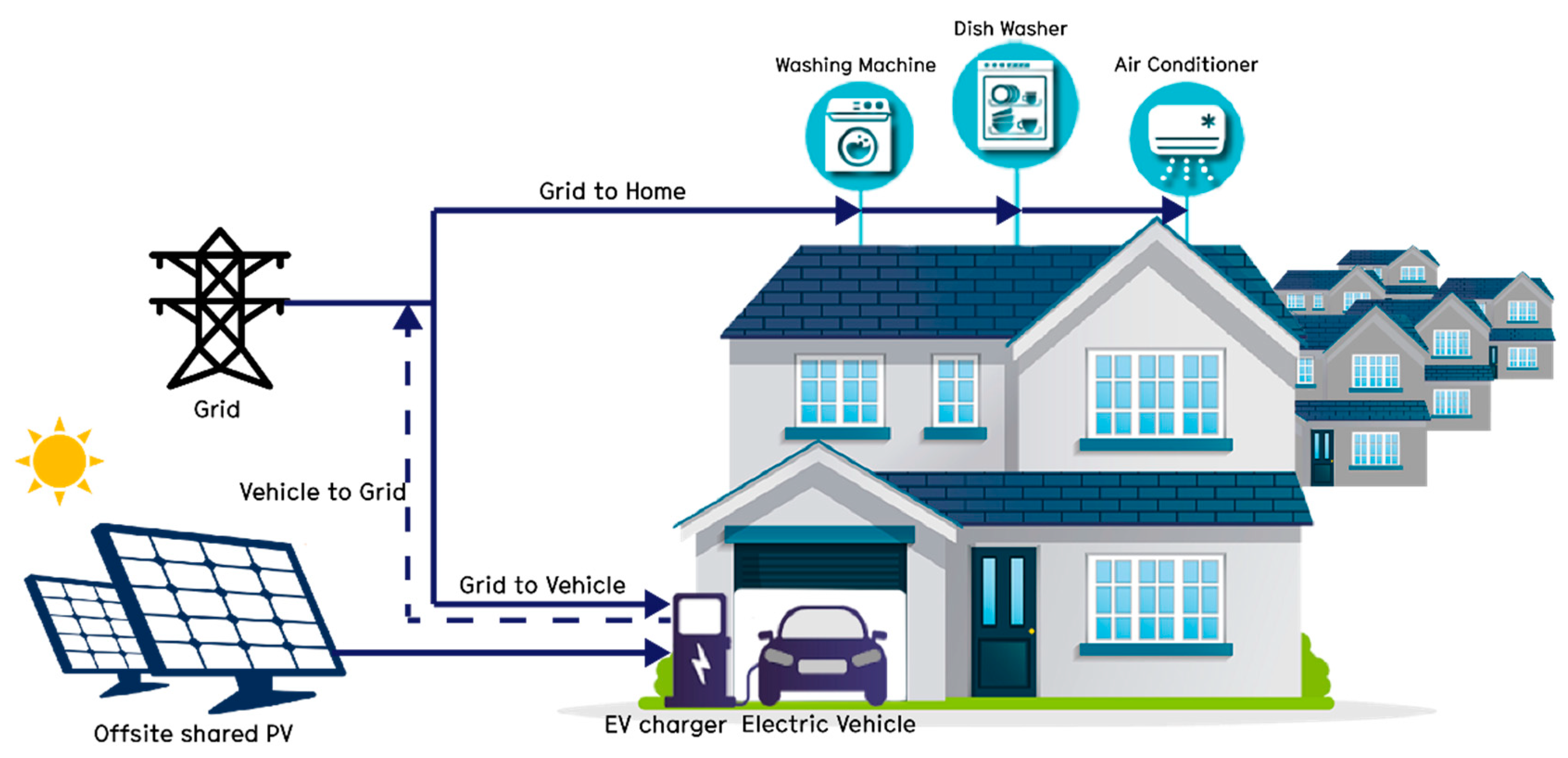
3. HEMS Model for the Residential Community
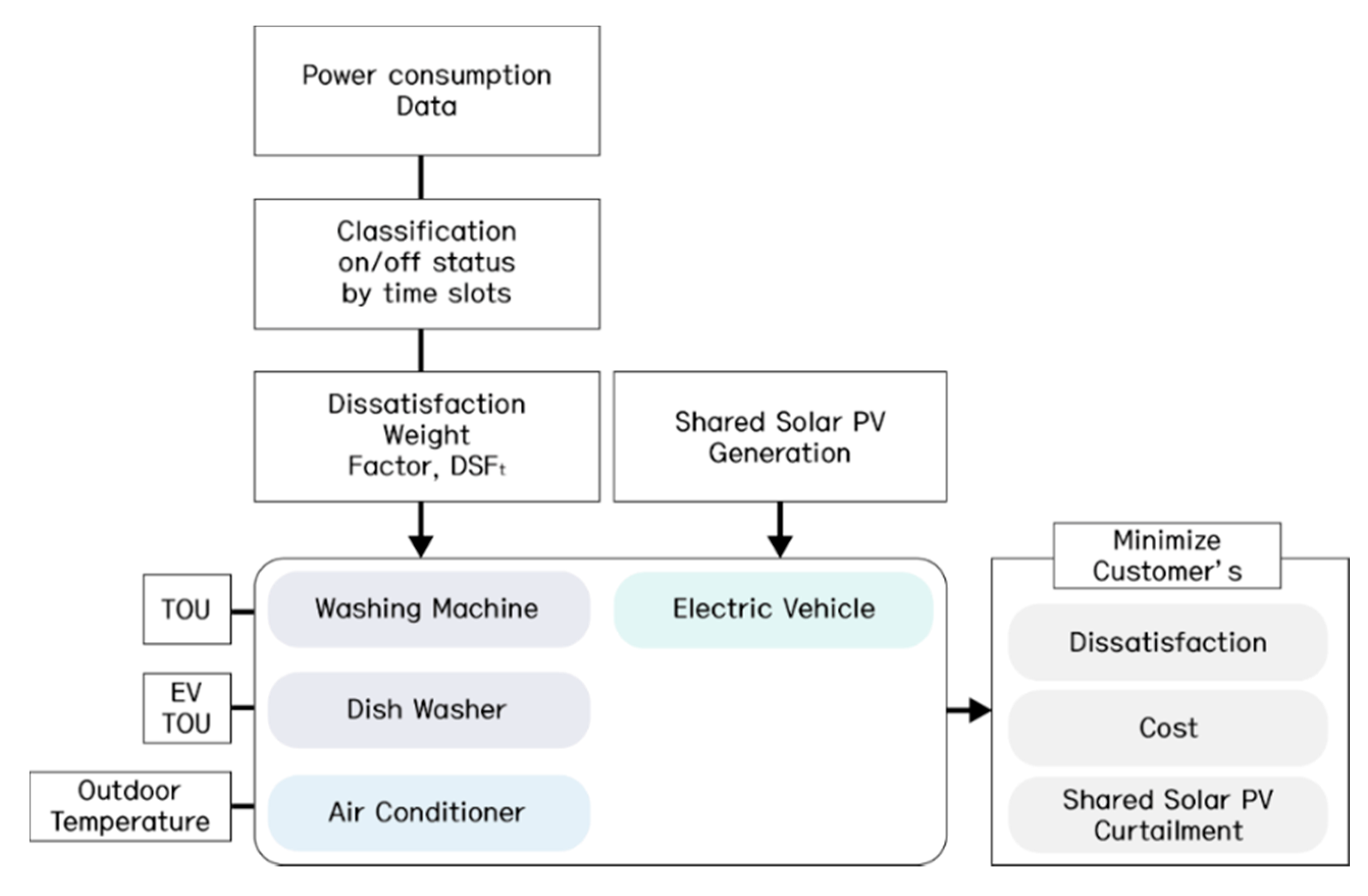
Figure 1 describes the HEMS model for the residential community. Each residential customer has home appliances washing machine (wm), dish washer (dw), air conditioner (ac), and EV. All the residential houses use a shared solar PV and the electricity generated is sent to the home charger when the residential EV user requires charging. The maximum capacity that an EV user can charge with the electricity generated from the PV is the total amount of PV divided by the number of households. The customer can also make a profit by selling the electricity through the discharge. Furthermore, the EV user will save the cost by discharging to the grid. Figure 2 shows an overall flowchart of HEMS optimization considering the shared PV power, TOU tariff scheme, and setting the dissatisfaction weight from real energy consumption data.

4. Methodology

4.1. Mathematical Modeling

In this section, the mathematical formulations of the proposed HEMS model are shown. Firstly, the multi-objective optimization constraints of home appliances and EV is presented. Next, the contents of setting the customer’s dissatisfaction weight and parameters are shown. Finally, the multi-objective optimization function is shown.

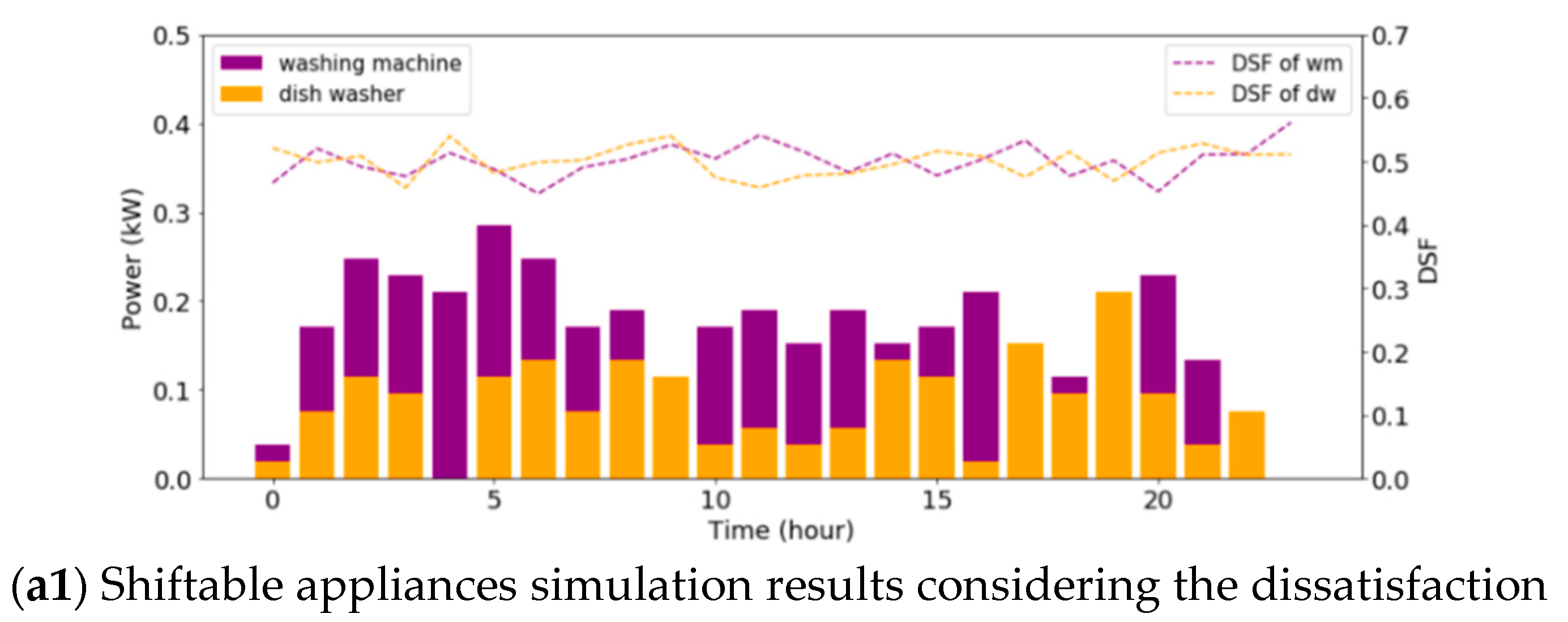
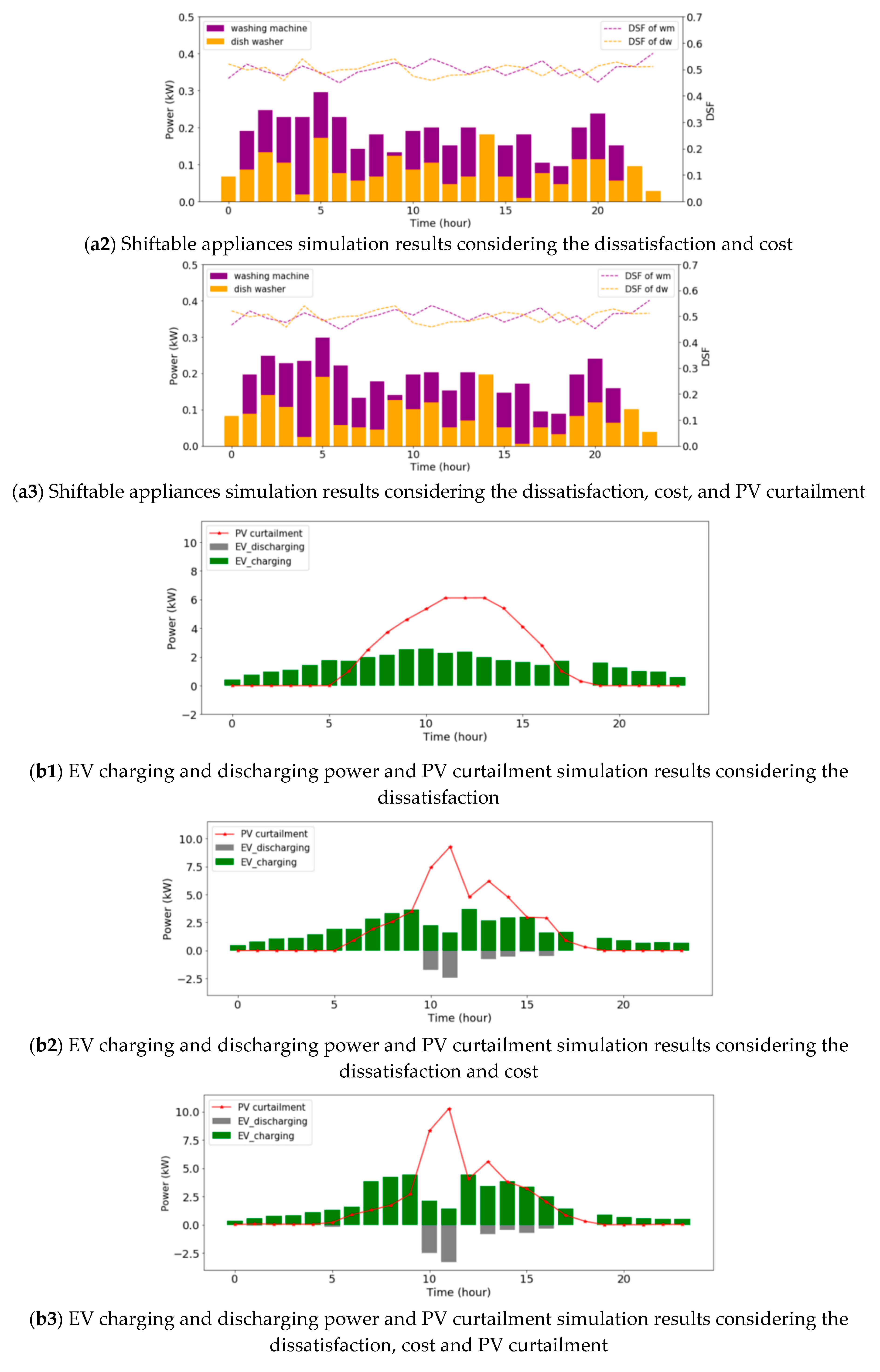
4.1.1. Shiftable Appliances

Equations (1)–(3) express the models of shiftable appliances. Equation (1) shows the optimized power consumption of appliances i at time t . Equation (2) presents the on/off operation state of the appliances. Shiftable appliances have a fixed operation time γ , which is running for γ hours from the time it is started Equation (3).
P t i = X t i P r a t e d i   i { w m ,   d w } ,   t T
X t i = { 0     i   { w m ,   d w } , t T w o r k i 1     i   { w m ,   d w } , t T w o r k i
t t + γ i 1 X t i = γ i ,   i   { w m ,   d w } ,   t T

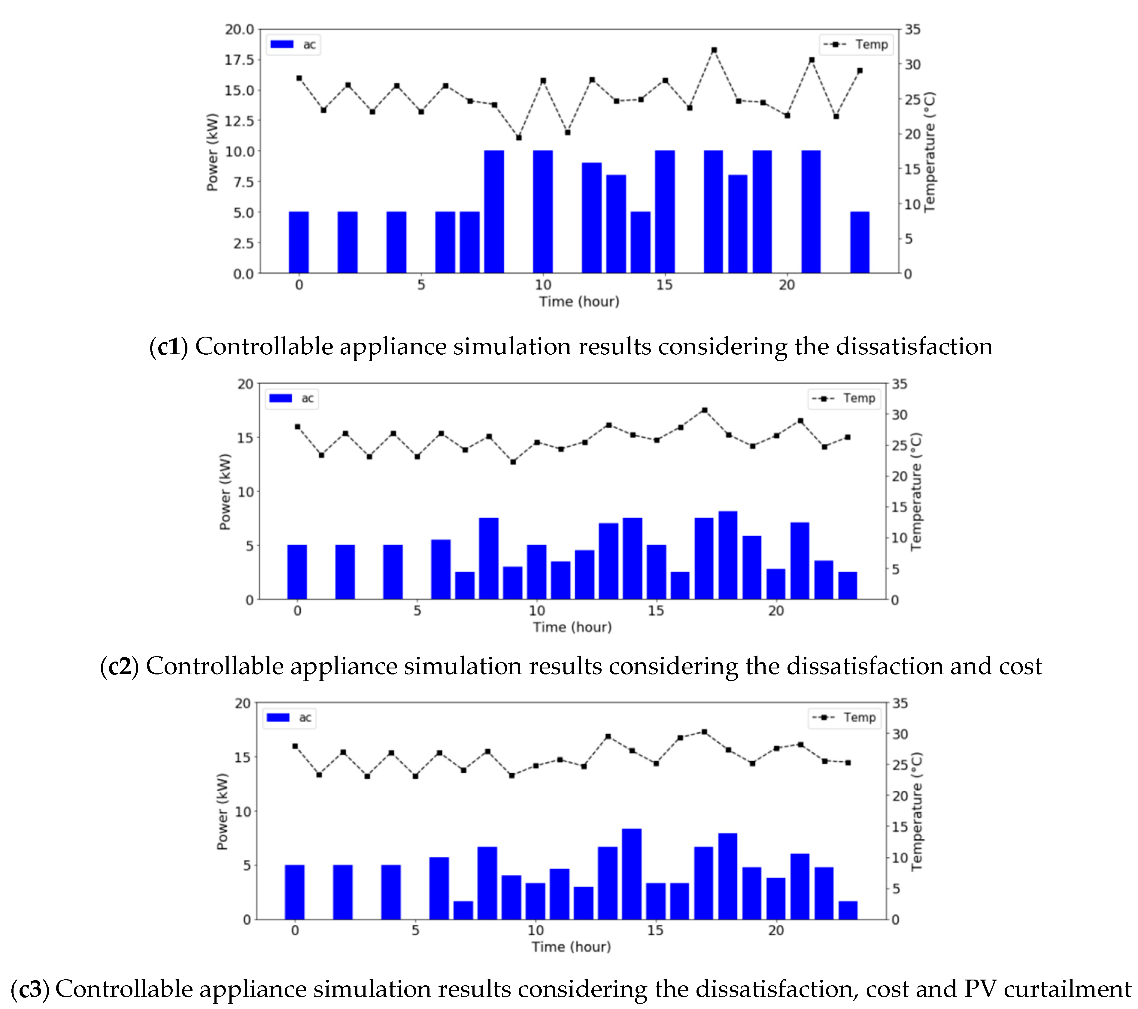
4.1.2. Controllable Appliance

The model of an air conditioner, which is classified as a power controllable appliance is shown in Equations (4)–(9). In Equation (4), where θ t + 1 i n is the indoor temperature at time t + 1 , this temperature is calculated by outdoor temperature at time t and efficiency of appliances η a c and power consumption P t a c . A residential customer sets the preference temperature θ p r e f e r i n in Equation (7). Depending on the customer’s preference temperature, the HEMS model optimizes the power consumption level as in Equation (8) and conducts scheduling on/off states as in Equation (6).
θ t + 1 i n = ε · θ t i n + ( 1 ε ) · ( θ t o u t η a c · P t a c ) ,   t T
P t a c = X t P a c , r a t e d ,   t T
X t a c = { 0 ,   θ t i n θ p r e f e r i n 1 ,   θ t i n > θ p r e f e r i n , t T
θ p r e f e r i n = 25  
P a c , m i n P a c , r a t e d P a c , m a x
θ i n i i n = θ t = 0 o u t

4.1.3. Interruptible Appliance

The mathematical modeling of an EV, which is classified as an interruptible appliance of the proposed HEMS model is given in Equations (10)–(19). The departure and arrival times of the EV are kept open in all the time slots so that they can be optimized based on the customer’s pattern.
P t e v ( t ) = X t e v P t e v , r a t e d , t [ T a = 19 ,   T d = 18 ]
X t e v = { 1 ,     c h a r g i n g   s t a t e ,   P t e v = P t e v , r a t e d , t [ T a , T d ] 0 ,     s t e a d y   s t a t e , 1 ,     d i s c h a r g i n g   s t a t e ,   P t e v = P t e v , r a t e d , t [ T a , T d ]
S O C t = S O C i n i ,   i f   t = T a
S O C t = S O C m a x ,   i f   t = T d
X t e v = 0 ,   i f   t = T d
S O C t = S O C t 1 + η c P c Δ T E c a p η d c P d c Δ T E c a p ,   t ( T a , T d )
S O C m i n S O C t S O C m a x
0 P t c η c P c h , m a x
0 P t d c η d c P d c h , m a x
P t e v , r a t e d = 2 , 4 , 6   kWh

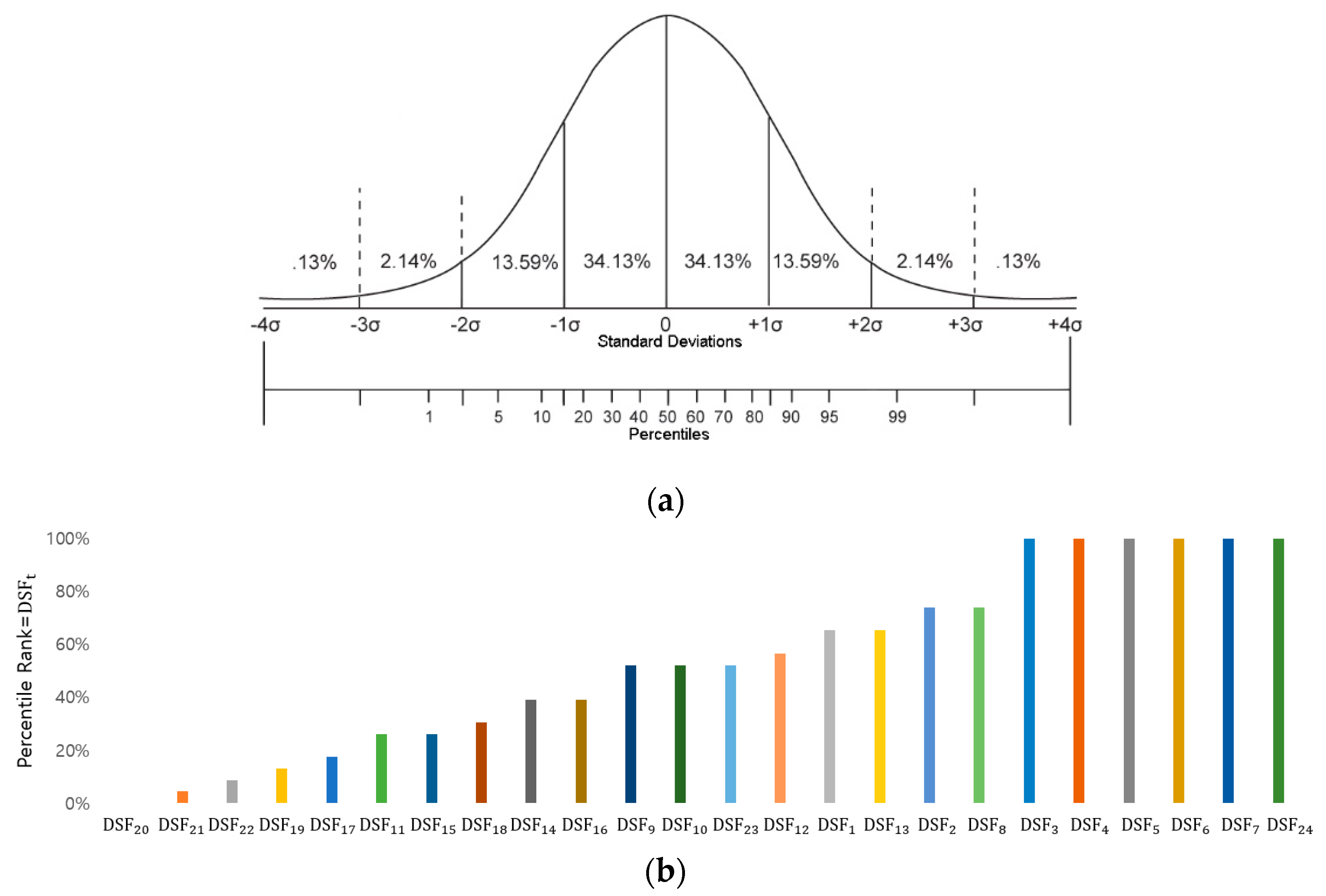
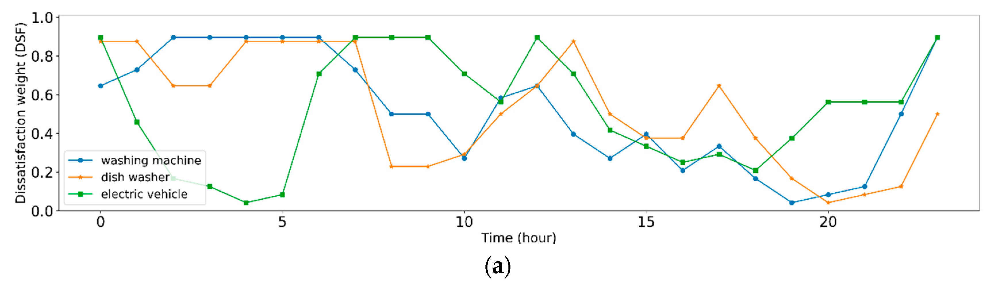
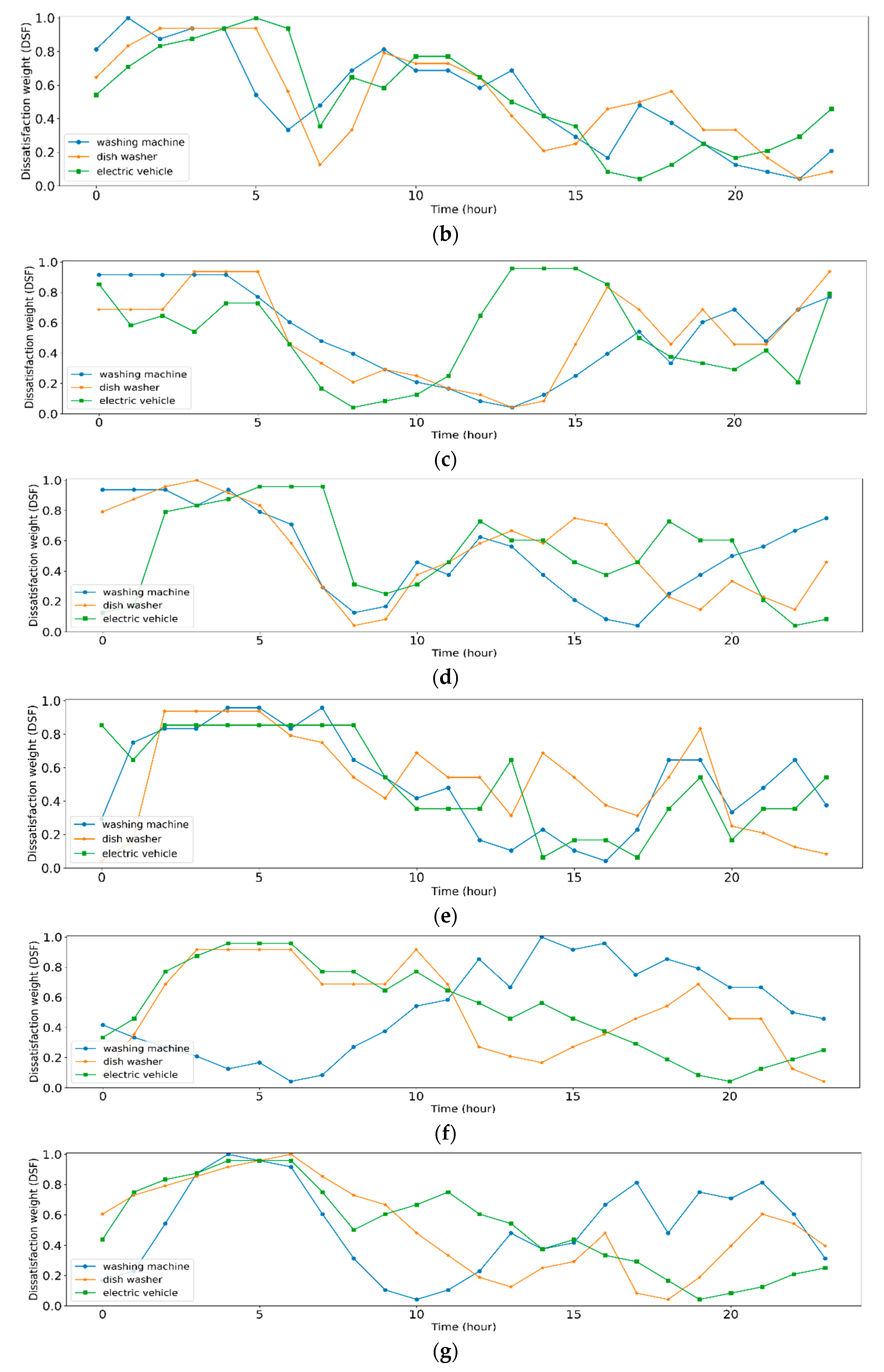
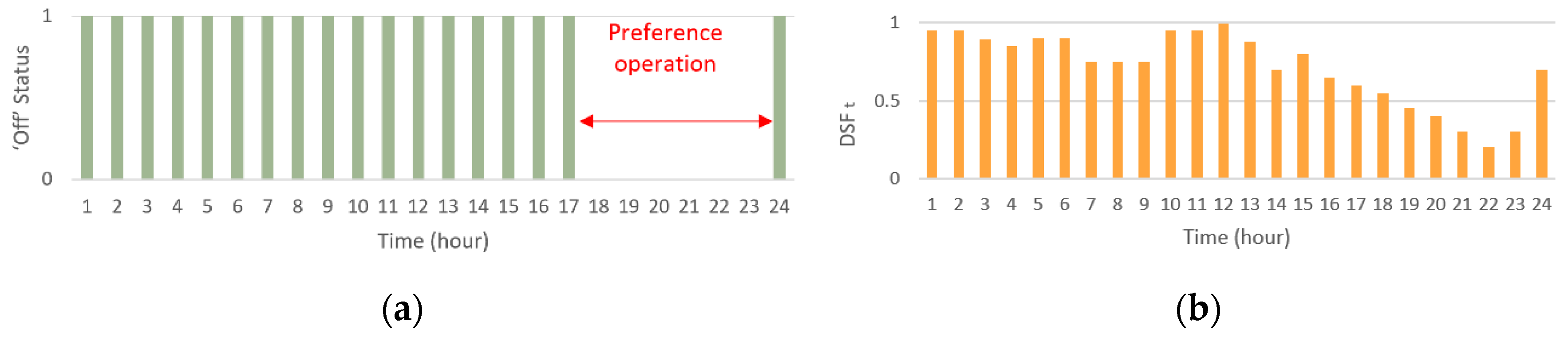
4.1.4. Setting the Dissatisfaction Weight

For the proposed HEMS model analysis, the Pecan Street data [29] consisting of energy consumption data for 7 residential customers from Austin, Texas in 2018 were used. Determination of the on/off states of the appliances was achieved by using only the power consumption data as provided in [30]. An analysis of the power consumption of the appliances during the weekdays of the year showed that the metering data is extremely low on the power consumption scale of each appliance as they are ‘off’ most of the time, and hence, most of the readings are near zero. Therefore, the on/off state of the home appliance at time t on day d is   S ( x t , d ) , and it is set to ‘on’ when the energy consumption data at time t on day d, x t , d is much greater than 1 standard deviation σ x t , D from the mean of the whole weekdays of D at time t, x ¯ t , D as in Equation (20).
S ( x t , d ) = { 1 , x t , d x ¯ t , D + σ x t , D 0 , x t , d < x ¯ t , D + σ x t , D
Then, the probability value at which the appliance is ‘on’ at time t, R t , where R t denotes the total sum of S ( x t , d ) during the whole weekdays of D, which is divided by the total number of weekdays is defined as in Equation (21).
R t = d D S ( x t , d ) n ( D )
DSF t : The dissatisfaction weight at time t can be denoted by the percentile rank given in Equation (22), and [31]. The probability value that the appliance’s state is ‘off’ is defined as 1 R t at time t.
DSF t = c l + 0.5 n ( 1 R t ) n ( T ) × 100 % ,     T = [ 0 ,   1 ,   ,   23 ]
In [31], where c l denotes the count of all the values less than the value of interest, that is 1 R t is the frequency of the value of interest and n ( T ) is the number of time slots in day d.
Figure 3a with normal bell-shaped curve and standard deviation value shows that percentile rank represents the ratio of the probability of appliances use from the top 0% to the bottom 100%. The definition of percentile rank used in this study has a lower percent value and a smaller percent value. Figure 3b shows that 8 p.m. is the most preferred appliance usage time among all 24 periods. Figure 3b lists DSF t values in small order, and Figure 4 below is a graph showing DSF t values by time slot of the 7 households.
Through the process described in Equations (20)–(22), the dissatisfaction weights of each time slot were derived. When the dissatisfaction weight is small at time t, it means that the residential customer has a greater probability of using the appliance at time t compared to the other time. In addition, the energy consumption patterns by time slots appeared similarly and differently for each appliance. It is presumed that this result is because there is no one present in the house. In this study, shiftable and interruptible appliances are used to determine the time at which an increase or a decrease in the customer’s dissatisfaction occurs. The results of the analysis of the dynamic changes in costs are shown in Figure 5 and Table 1. In previous studies [13,19,20,21,22,32,33], binary or integer dissatisfaction values were used based on the preferred appliance usage time or on/off state changes. The proposed model reflected the patterns of actual customers with less rigidity differences in dissatisfaction over time, and it was observed that the customers using the TOU tariff were more actively saving costs. The proposed model is more reasonable in terms of optimal scheduling for cost saving of shiftable and interruptible appliances. However, the degree of dissatisfaction for the power controllable appliance is determined by indoor temperature and not by the customer’s appliance usage time.

4.1.5. Parameters

For EV tariff is shown in Figure 6, the maximum discharging tariff was assumed is set at 130% of the maximal charging tariff, and the minimum discharging tariff was set at 60% of the minimal charging tariff with reference to [34].
The parameters of the appliances are given in Table 2. It is assumed the operation duration of the appliance is 2 h for the washing machine and 1 h for the dishwasher. The air conditioner is consumed with a power in the range of 5 to 10 kWh depending on the preference temperature. The battery capacity of the electric vehicle is 60 kWh, the maximum SOC of the battery is set to be 0.85, and the minimum SOC of the battery is set to be 0.1. Charging and discharging power can be variously output as 2, 4, and 6 kWh.

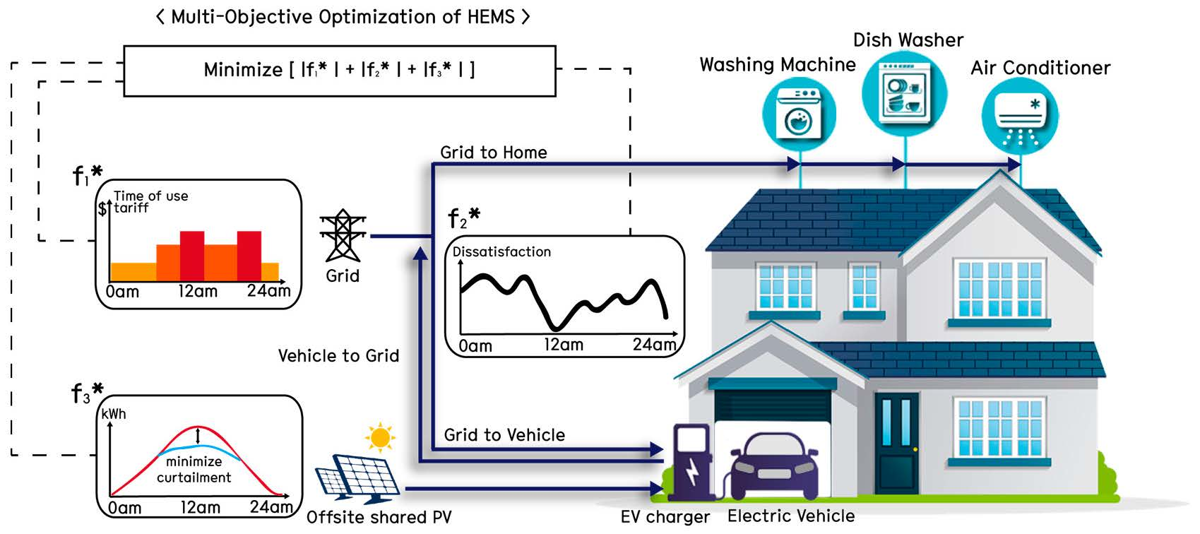
4.2. Multi-Objective Function

In this section, the multi-objective optimization of the proposed HEMS model is solved using the mixed-integer linear program (MILP) algorithm using IBM ILOG studio with the CPLEX solver [35,36]. The HEMS optimization model is introduced to minimize the cost of the residential customers and minimize the curtailment of the PV, which is jointly invested in by the residential community.

4.2.1. Multi-Objective Function

The multi-objective optimization function consists of three parts. The first optimization function f 1 is the total electricity consumption in Equation (23). If the demand of the EV charging exceeds generation of PV, the cost paid depends on the electricity pricing structure in Equation (23a). On the other hand, if the power generation exceeds the EV charging, the cost is calculated as in Equation (23b).
f 1 = { (23a) t T { π t ( P t a c + P t w m + P t d w ) + π t e v , c h a ( P t e v , c h a P t P V ) π t e v , d c h P t e v , d c h } ,   i f   P t e v , c h a > P t P V (23b) t T { π t ( P t a c + P t w m + P t d w ) π t e v , d c h P t e v , d c h } ,   i f   P t e v , c h a P t P V
The second optimization function f 2 aims to minimize the dissatisfaction of the residential customer. X t B L , i is the binary variable of appliance i’s state at time t, and only the dissatisfaction is considered. That is, the scheduled state is set as a baseline from the real consumption data. So f 2 is composed of the difference between the baseline ( X t B L , i ) and the scheduled state ( X t o p t , i ), and the dissatisfaction weights for each time slot in Equation (24).
f 2 = i { e v , w m , d w } t T { | X t B L , i X t o p t , i | × DSF t , i }
The third objective function is given in Equation (25). Residential customer optimizes scheduling of EV charging to reduce PV curtailment while considering individual costs and dissatisfaction.
f 3 = t T | P t P V P t e v , c |

4.2.2. Normalization

Each of the multi-objective optimization functions has different units and different orders of magnitude. Hence, it is necessary to normalize them such that they all have similar magnitudes [35]. The multi-objective functions f 1 * ,   f 2 * ,   and   f 3 * were normalized as in Equations (26)–(28) to assume a value between 0 and 1.
f 1 * ( x ) = [ f 1 ( x ) min f 1 ( x ) max f 1 ( x ) min f 1 ( x ) ]
f 2 * ( x ) = [ f 2 ( x ) min f 2 ( x ) max f 2 ( x ) min f 2 ( x ) ]
f 3 * ( x ) = [ f 3 ( x ) min f 3 ( x ) max f 3 ( x ) min f 3 ( x ) ]
The Multi-Objective function is as follows:
Minimize   [ | f 1 * | + | f 2 * | + | f 3 * | ]

4.2.3. Priority Method

Many solutions to the multi-objective optimization method are available, and there is no single correct answer [37,38]. The CPLEX can automatically generate priority orders, that determine the optimal variable point. The priority method has an order of importance for each objective function and it simulates by changing the order for all of them.

5. Analysis of the Results

5.1. Case Results at EV Battery Capacity 36 kWh

This section is divided into three scenarios of different objective functions showing the scheduling results by appliance type such as shiftable, interruptible, and controllable. To analyze the results of the HEMS simulation with various patterns of data, the dissatisfaction weights of 105 residential households were generated using a random number generation method. The average values for the scheduling results of the households are summarized. The proposed dissatisfaction weight model to analyze the optimal scheduling that considered the dissatisfaction of the residential customer was applied. The scheduling that considered only the dissatisfaction using the energy consumption data was considered as the baseline Figure 7(a1,b1,c1). This model assumes that the customer’s plan to reduce the TOU tariff or reduce the PV curtailment is not reflected. Figure 7(a2,b2,c2) shows an optimized scheduling result that considered cost and dissatisfaction. The results for minimizing the PV curtailment in addition to cost and dissatisfaction can be seen in Figure 7(a3,b3,c3).
The results of the shiftable appliance in Figure 7 show that the appliance is used even though the DSF is high in Figue 7(a2,a3), unlike in Figure 7(a1). There was no significant change in the scheduling difference between Figure 7(a2,a3). The interruptible appliance results show that in Figure 7(b2,b3), the frequent discharges during the daytime are with the high discharge tariff. In the case of Figure 7(b3), it is seen that it charges more than (b2) to minimize the PV curtailment. In the case of the power controllable appliance as in Figure 7(c3), the average power value by time slot was low, and the average temperature was higher than in the other cases Figure 7(c1,c2).
By comparing the results of the three approaches when the EV battery capacity is numerically 36 kWh, in case 1, the cost, dissatisfaction, and the amount of PV curtailment were US$18.77, 0.13, and 59.48 kWh, respectively. However, when the residential customers considered cost saving in case 2, the cost was US$10.34, a decrease of US$8.43 from case 1. However, dissatisfaction increased from 0.13 to 2.61. In the scheduling results of case 3, dissatisfaction increased and PV curtailment decreased when compared to both cases 1 and 2. The cost also decreased by US$0.89 from US$10.34 in case 2 to US$9.45. When the battery capacity is 36 kWh, the discharge was maintained at the time of the highest discharge tariff and the charge was increased in the rest of the time to minimize the PV curtailment.

5.2. Case Results by Various EV Battery Capacities

The results of the three cases for each EV battery capacity were analyzed in Table 3 and it was confirmed that the cost increased again in case 3 when the capacity is 60 kWh or more. This analysis shows that the EV battery capacity is directly proportional to the charging time and power required. Furthermore, as the EV battery capacity increases, the opportunity cost for the discharge increases, and thus, a minimum incentive cost is required to minimize PV curtailment. When the capacities of 36 and 84 kWh, in case 3 and case 2 are compared, the PV curtailment decreased by 5.6 and 6.3, respectively. A customer with an 84 kWh battery will not try to minimize PV curtailment because of higher cost. Therefore, a minimum incentive should be ensured, which is above the difference of US$14.58 in case 3 and US$14.27 in case 2.

6. Discussion and Conclusion

This study is motivated by the aforementioned research works based on a multi-objective HEMS. The major contribution of this paper is summarized as follows:
  • Multi-objective optimal scheduling considering cost and dissatisfaction by using the On/Off pattern for each appliance as the dissatisfaction weight for each time slot.
Many previous HEMS studies have considered consumer dissatisfaction, however, the preference time and binary index of dissatisfaction were based on assumptions. Previously, the subjective factor, that is, the consumer’s discomfort was not expressed correctly. The weight of dissatisfaction is determined through real power consumption data. The preference for each time slot, which is not strictly classified as a binary index or an integer, resulted in more aggressive cost reduction.
  • It is proposed to optimize scheduling of EV charging and minimizing the cost and dissatisfaction of individuals with the aim of minimizing the curtailment of PV shared by multiple households.
The opportunity cost of discharge for each residential customer’s specific battery capacity is estimated. An appropriate incentive range to be paid according to the capacity of the EV battery is derived. Based on this, the system operator can induce EV charging to reduce PV curtailment.
The optimal scheduling model was proposed taking into account the customer’s dissatisfaction, cost, and PV curtailment in this study. Here, the customer’s dissatisfaction weight was included only with respect to the energy consumption data. In a previous study, the binary or integer weight approach was utilized making dynamic scheduling for cost saving difficult [13,19,20,21,22,32,33]. The MILP optimization through this model brought about a more aggressive cost reduction effect while considering the actual residential customer’s usage patterns. Also, it was proved that the plan to use PV generation through EV charging affects the cost of the customers. By utilizing PV power generation to charge EV battery, it is possible to recover the investment cost of the solar community, because power from utility was saved for EV charges during peak load periods. Besides, it helps to mitigate the duck curve caused by the large amount of PV power generation to provide flexibility of the power system instead of PV curtailment. The important key factor is EV battery capacities in this study. EV charging power size is the same as 2, 4, and 6 kWh, but EV batteries have various capacities. The EV battery capacity affects the scheduling of charging and discharging and PV curtailment. If EV battery capacity is small (e.g., less than 60 kWh), EV owner tends to charge using PV power generation to maintain certain SOC level. Otherwise, EV owner tends to discharge power of EV battery instead of charging PV power generation. Therefore, we concluded that the HEMS optimization scheduling strategy according to the EV battery capacity should also be changed. In the future, an in-depth analysis of the results of cases 2 and 3, with respect to the TOU tariff and the appropriate selling price of the discharge to induce EV charging in the period of high PV generation will be conducted, and the EV TOU design will be evaluated considering incentives.

Author Contributions

Y.K. conceived the idea for the research and formulated the research problem. T.K. helped to do experiment and checked the algorithm. Y.K. and K.B. proposed the mathematical model. J.K. led and supervised the research and is the corresponding author. All authors have read and agreed to the published version of the manuscript.

Funding

This research received no external funding.

Acknowledgments

This work was supported by the Korea Institute of Energy Technology Evaluation and Planning (KETEP) and the Ministry of Trade, Industry and Energy (MOTIE) of the Republic of Korea (No. 20181210301380).

Conflicts of Interest

The authors declare no conflict of interest.

Nomenclature

SymbolDescription
HEMSHome Energy Management System
TOU tariffTime of Use tariff
EVElectric Vehicle
PVPhotovoltaic
π t 
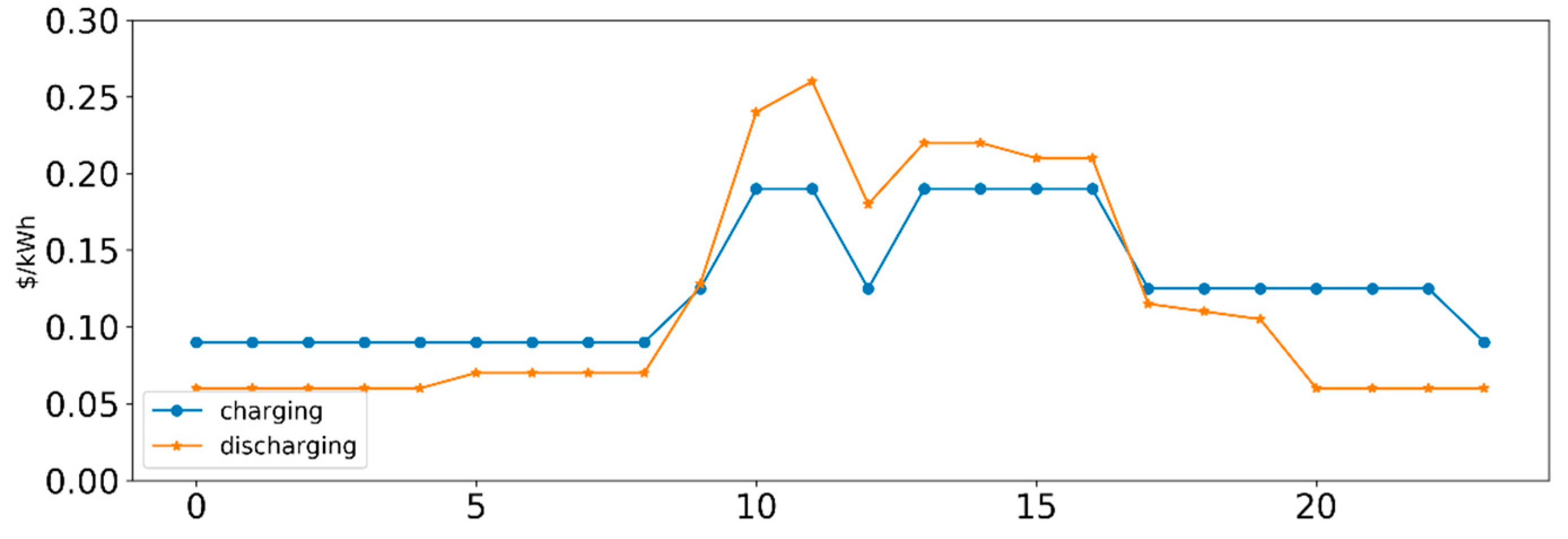
Electricity price at time t
π t e v , c Electric vehicle charging price at time t
π t e v , d c Electric vehicle discharging selling price at time t
X t i on/off status of appliance i at time t
X t B L , i Real energy consumption data based appliance on/off states
X t o p t , i Optimized appliance’s on/off status
P t i Optimal power of appliance i at time t
T w o r k i Time slot in which the appliance i was worked
γ i Shiftable appliance i operating time
S ( x t , d ) the on/off state of the home appliance at time t on day d
x ¯ t , D mean value of appliance energy consumption data at time t on day d
σ x t , D standard deviation of appliance energy consumption data at time t on day d
R t the probability value that the appliances is ‘on’ at time t
DSF t the dissatisfaction weight at time t
θ t i n Indoor temperature
θ p r e f e r i n Customer preferred temperature
θ t o u t Outdoor temperature
ε System inertia of air conditioner
η a c Efficiency of air conditioner
P t e v , c h a Electric vehicle charging power at time t
P t e v , d c h Electric vehicle discharging power at time t
S O C t State of charge of electric vehicle at time t
S O C i n i Initial state of charge of electric vehicle
S O C m a x Maximum state of charge of electric vehicle
S O C m i n Minimum state of charge of electric vehicle
E c a p Electric vehicle battery capacity
η c Electric vehicle charging efficiency
η d c Electric vehicle discharging efficiency
T a Electric vehicle arriving time
T d Electric vehicle departure time
wmShiftable appliance—washing machine
dwShiftable appliance—dish washer
evInterruptible appliance—electric vehicle
acControllable appliance—air conditioner

References

  1. Almusaylim, Z.A.; Zaman, N. A review on smart home present state and challenges: Linked to context-awareness internet of things (IoT). Wirel. Netw. 2018, 25, 3193–3204. [Google Scholar] [CrossRef]
  2. Khedekar, D.C.; Truco, A.C.; Oteyza, D.A.; Huertas, G.F. Home Automation-A Fast-Expanding Market. Thunderbird Int. Bus. Rev. 2017, 59, 79–91. [Google Scholar] [CrossRef]
  3. Chauhan, A.S. How AI Is Transforming Home Automation. Available online: https://becominghuman.ai/how-ai-is-transforming-home-automation-56085cb275b (accessed on 4 April 2020).
  4. Ejaz, W.; Naeem, M.; Shahid, A.; Anpalagan, A.; Jo, M. Efficient energy management for the internet of things in smart cities. IEEE Commun. Mag. 2017, 55, 84–91. [Google Scholar] [CrossRef] [Green Version]
  5. Yoldaş, Y.; Önen, A.; Muyeen, S.M.; Vasilakos, A.V.; Alan, İ. Enhancing smart grid with microgrids: Challenges and opportunities. Renew. Sustain. Energy Rev. 2017, 72, 205–214. [Google Scholar] [CrossRef]
  6. Phuangpornpitak, N.; Tia, S. Opportunities and Challenges of Integrating Renewable Energy in Smart Grid System. Energy Procedia 2013, 34, 282–290. [Google Scholar] [CrossRef] [Green Version]
  7. Uribe-Pérez, N.; Hernández, L.; de la Vega, D.; Angulo, I. State of the Art and Trends Review of Smart Metering in Electricity Grids. Appl. Sci. 2016, 6, 68. [Google Scholar] [CrossRef]
  8. Tan, K.M.; Ramachandaramurthy, V.K.; Yong, J.Y. Integration of electric vehicles in smart grid: A review on vehicle to grid technologies and optimization techniques. Renew. Sustain. Energy Rev. 2016, 53, 720–732. [Google Scholar] [CrossRef]
  9. Benefits of Demand Response in Electricity Markets and Recommendations for Achieving Them; U.S. Department of Energy: Washington, DC, USA, 2006.
  10. Paranjape, Z.W.U.M.R. Stochastic Optimization for Residential Demand Response under Time of Use. In Proceedings of the IEEE International Conference on Power Electronics, Smart Grid and Renewable Energy (PESGRE2020), Cochin, India, 2–4 January 2020. [Google Scholar]
  11. Zhao, L.; Yang, Z.; Lee, W.-J. The Impact of Time-of-Use (TOU) Rate Structure on Consumption Patterns of the Residential Customers. IEEE Trans. Ind. Appl. 2017, 53, 5130–5138. [Google Scholar] [CrossRef]
  12. Hussain, H.; Javaid, N.; Iqbal, S.; Hasan, Q.; Aurangzeb, K.; Alhussein, M. An Efficient Demand Side Management System with a New Optimized Home Energy Management Controller in Smart Grid. Energies 2018, 11, 190. [Google Scholar] [CrossRef] [Green Version]
  13. Veras, J.M.; Silva, I.R.S.; Pinheiro, P.R.; Rabelo, R.A.L.; Veloso, A.F.S.; Borges, F.A.S.; Rodrigues, J. A Multi-Objective Demand Response Optimization Model for Scheduling Loads in a Home Energy Management System. Sensors 2018, 18, 3207. [Google Scholar] [CrossRef] [Green Version]
  14. Zhu, Z.; Tang, J.; Lambotharan, S.; Chin, W.H.; Fan, Z. An Integer Linear Programming and Game Theory Based Optimization for Demand Side Management in Smart Grid. In Proceedings of the 2011 IEEE GLOBECOM Workshops (GC Wkshps), Houston, TX, USA, 5–9 December 2011; pp. 1205–1210. [Google Scholar]
  15. Parida, B.; Iniyan, S.; Goic, R. A review of solar photovoltaic technologies. Renew. Sustain. Energy Rev. 2011, 15, 1625–1636. [Google Scholar] [CrossRef]
  16. Nguyen, D.T.; Le, L.B. Joint Optimization of Electric Vehicle and Home Energy Scheduling Considering User Comfort Preference. IEEE Trans. Smart Grid 2014, 5, 188–199. [Google Scholar] [CrossRef]
  17. Shoji, T.; Hirohashi, W.; Fujimoto, Y.; Hayashi, Y. Home Energy Management Based on Bayesian Network Considering Resident Convenience. In Proceedings of the 2014 International Conference on Probabilistic Methods Applied to Power Systems (PMAPS), Durham, UK, 7–10 July 2014; IEEE: Durham, UK, 2014; pp. 1–6. [Google Scholar]
  18. Rastegar, M. Impacts of Residential Energy Management on Reliability of Distribution Systems Considering a Customer Satisfaction Model. IEEE Trans. Power Syst. 2018, 33, 6062–6073. [Google Scholar] [CrossRef]
  19. Zhu, J.; Lin, Y.; Lei, W.; Liu, Y.; Tao, M. Optimal household appliances scheduling of multiple smart homes using an improved cooperative algorithm. Energy 2019, 171, 944–955. [Google Scholar] [CrossRef]
  20. Joo, I.-Y.; Choi, D.-H. Optimal household appliance scheduling considering consumer’s electricity bill target. IEEE Trans. Consum. Electron. 2017, 63, 19–27. [Google Scholar] [CrossRef]
  21. Khan, A.; Javaid, N.; Khan, M.I. Time and device based priority induced comfort management in smart home within the consumer budget limitation. Sustain. Cities Soc. 2018, 41, 538–555. [Google Scholar] [CrossRef]
  22. Li, K.; Zhang, P.; Li, G.; Wang, F.; Mi, Z.; Chen, H. Day-Ahead Optimal Joint Scheduling Model of Electric and Natural Gas Appliances for Home Integrated Energy Management. IEEE Access 2019, 7, 133628–133640. [Google Scholar] [CrossRef]
  23. Tushar, M.H.K.; Assi, C.; Maier, M.; Uddin, M.F. Smart microgrids: Optimal joint scheduling for electric vehicles and home appliances. IEEE Trans. Smart Grid 2014, 5, 239–250. [Google Scholar] [CrossRef]
  24. Aoun, A.; Ibrahim, H.; Ghandour, M.; Ilinca, A. Supply Side Management vs. Demand Side Management of a Residential Microgrid Equipped with an Electric Vehicle in a Dual Tariff Scheme. Energies 2019, 12, 4351. [Google Scholar] [CrossRef] [Green Version]
  25. He, Y.; Venkatesh, B.; Guan, L. Optimal Scheduling for Charging and Discharging of Electric Vehicles. IEEE Trans. Smart Grid 2012, 3, 1095–1105. [Google Scholar] [CrossRef]
  26. Rastegar, M.; Fotuhi-Firuzabad, M.; Moeini- Aghtaie, M. Developing a Two-Level Framework for Residential Energy Management. IEEE Trans. Smart Grid 2016, 9, 1707–1717. [Google Scholar] [CrossRef]
  27. Ioakimidis, C.S.; Thomas, D.; Rycerski, P.; Genikomsakis, K.N. Peak shaving and valley filling of power consumption profile in non-residential buildings using an electric vehicle parking lot. Energy 2018, 148, 148–158. [Google Scholar] [CrossRef]
  28. Ito, A.; Kawashima, A.; Suzuki, T.; Inagaki, S.; Yamaguchi, T.; Zhou, Z. Model Predictive Charging Control of In-Vehicle Batteries for Home Energy Management Based on Vehicle State Prediction. IEEE Trans. Control. Syst. Technol. 2018, 26, 51–64. [Google Scholar] [CrossRef]
  29. Kikusato, H.; Mori, K.; Yoshizawa, S.; Fujimoto, Y.; Asano, H.; Hayashi, Y.; Kawashima, A.; Inagaki, S.; Suzuki, T. Electric Vehicle Charge–Discharge Management for Utilization of Photovoltaic by Coordination Between Home and Grid Energy Management Systems. IEEE Trans. Smart Grid 2019, 10, 3186–3197. [Google Scholar] [CrossRef]
  30. Pecan Street. Available online: https://www.pecanstreet.org/dataport/ (accessed on 9 October 2019).
  31. Tang, Y.; Sakai, K.; Luo, S.; Zhao, Y. AI in Depth: Monitoring Home Appliances from Power Readings with ML. Available online: https://cloud.google.com/blog/products/ai-machine-learning/monitoring-home-appliances-from-power-readings-with-ml (accessed on 30 November 2019).
  32. WIKIPEDIA Percentil Rank. Available online: https://en.wikipedia.org/wiki/Percentile_rank (accessed on 10 January 2020).
  33. Setlhaolo, D.; Xia, X.; Zhang, J. Optimal scheduling of household appliances for demand response. Electr. Power Syst. Res. 2014, 116, 24–28. [Google Scholar] [CrossRef]
  34. Ma, Y.; Houghton, T.; Cruden, A.; Infield, D. Modeling the Benefits of Vehicle-to-Grid Technology to a Power System. IEEE Trans. Power Syst. 2012, 27, 1012–1020. [Google Scholar] [CrossRef]
  35. Arif, S.M.; Lie, T.T.; Seet, B.C.; Ahsan, S.M.; Khan, H.A. Plug-In Electric Bus Depot Charging with PV and ESS and Their Impact on LV Feeder. Energies 2020, 13, 2139. [Google Scholar] [CrossRef]
  36. IBM ILOG CPLEX Optimization Studio. Available online: https://www.ibm.com/nl-en/products/ilog-cplex-optimization-studio (accessed on 5 February 2020).
  37. Arora, J.S. Multi-objective Optimum Design Concepts and Methods. In Introduction to Optimum Design; Elsevier: Cambridge, MA, USA, 2017; pp. 771–794. [Google Scholar]
  38. Yahia, Z.; Pradhan, A. Multi-objective optimization of household appliance scheduling problem considering consumer preference and peak load reduction. Sustain. Cities Soc. 2020, 55, 102058. [Google Scholar] [CrossRef]
Figure 1. Illustration of the Home Energy Management System (HEMS) model for the residential community.
Energies 13 02852 g001
Figure 2. Flowchart for the proposed HEMS model process.
Energies 13 02852 g002
Figure 3. (a) Percentile rank compared to a normal bell-shaped curve [31]; (b) Result of percentile rank for 24 h with R t value.
Energies 13 02852 g003
Figure 4. Seven households’ dissatisfaction weights (ag) with respect to each time slot.
Energies 13 02852 g004aEnergies 13 02852 g004b
Figure 5. (a) Simple dissatisfaction weight approach using binary values and (b) DSF t weight by each time slot of the proposed model.
Energies 13 02852 g005
Figure 6. Electric vehicle charging and discharging tariff profiles during each day.
Energies 13 02852 g006
Figure 7. (a) Simulation results of washing machine and dish washer (b) Simulation results of EV charging/discharging power and PV curtailment, and (c) Simulation results of air conditioner and indoor temperature.
Energies 13 02852 g007aEnergies 13 02852 g007bEnergies 13 02852 g007c
Table 1. Cost comparison according to the set dissatisfaction weight approach.
HouseBinary Optimal Cost ($/Day)Proposed Optimal Cost ($/Day)
#16.105.44
#26.465.56
#36.384.86
#45.955.42
#57.906.13
#66.075.41
#76.585.43
Table 2. Parameters of the appliances.
AppliancesPower (kWh)Operation Durations (h) Efficiency   η i
Washing Machine22-
Dish Washer21-
Air Conditioner5–10--
AppliancesCapacitySOCmaxSOCmin P t e v , c h a ,   P t e v ,   d c h η c ,   η d c
Electric Vehicle60 kWh0.850.12, 4, 6 kW0.9
Table 3. Comparison of results by EV battery capacities for the three cases.
CaseEV Battery Capacity (kWh)DissatisfactionCost ($/Day)PV Curtailment (kWh/Day)
1360.1318.7759.48
480.2919.8858.33
600.5020.4754.92
720.8221.1752.38
841.2321.7149.01
2362.6110.3451.99
482.9311.3850.13
603.5012.0547.01
723.5913.1444.99
843.6414.2743.12
3364.249.4545.69
484.3810.7742.80
604.0112.1539.92
723.8413.4537.92
843.7214.5837.51

