Abstract
This paper describes a system to support the development and assessment of methodologies that explore the energy flexibility provided by electric water heaters. The proposed system follows a modular approach and allows users to share and remotely control the referred devices. The operation of this system is presented in this paper considering a case study where the energy flexibility provided by a 100 L electric water heater is used to reduce electricity costs under the Portuguese tariff context. The collected results reveal that increasing the available energy flexibility leads to larger savings. These results also show that the referred savings depend on the instant associated to hot water consumption events.
1. Introduction
The concept of energy flexibility is receiving considerable attention worldwide, leading, for example, to the development of international projects like the IEA (International Energy Agency) and EBC (Energy in Buildings and Communities program) Annex 67. Buildings, in particular, which account for approximately 40% of energy consumption and 36% of CO2 emissions in the European Union [1], can provide energy flexibility to the demand side of power systems by allowing the control of specific devices, while respecting the comfort needs of the respective users [2].
Taking into consideration that in the European Union and in the United States of America, domestic hot water heating accounts for 14% and 17% of the electricity consumed in the residential sector [3], respectively, the energy flexibility offered by Electric Water Heaters (EWH) is of significant importance. Such flexibility is provided thanks to the thermal energy storage capabilities of EWH, being its control normally associated to the development of systems aimed to improve self-consumption of photovoltaic [4,5] and wind [6,7] generation or to reduce electricity related costs [8,9,10,11,12,13,14,15].
The literature [4,5,6,7,8,9,10,11,12,13,14,15] shows that there is a wide variety of methodologies being developed to exploit the energy flexibility provided by EWH while bringing benefits to users depending on specific objectives. For instance, EWH operation has been defined using genetic algorithms [4] or mixed integer linear programming techniques [5] to improve photovoltaic self-consumption. Regarding wind generation, external signals have been used both at individual and/or aggregated levels [6,7] to set the operation of EWH in order to increase matching between demand and the availability of the respective primary energy resource. Appliance commitment [8], dynamic programming [9], binary integer programming techniques [10], customer-centered heuristic [11], genetic algorithms [12], binary particle swarm optimization [13], reinforcement learning [9,14] and cost-optimal algorithms [15] have been used to support EWH operation and reduce associated electricity costs.
However, most of the assessment activities conducted in these studies are based on simulation, without considering possible challenges of real implementations (e.g., communication delays). Taking this into consideration, this paper describes a system entitled EFSyst (Energy Flexibility system) that aims to support the development and assessment of methodologies to explore the energy flexibility provided by EWH in real conditions. Given the number of possible methodologies to use this flexibility, EFSyst will also allow direct comparison between solutions in the same context. Additionally, this paper presents a case study to illustrate EFsyst operation and assess the benefits of using the referred flexibility to reduce the electricity costs associated to the operation of a 100 L EWH under the Portuguese electricity tariff context. Data associated to the experiments illustrating the EFsyst operation can be found in [16].
2. Developed System (EFsyst)
The EFsyst supports the development and assessment of methodologies to explore the energy flexibility provided by EWH considering real conditions and the inherent challenges that are not normally modeled in simulation environments (e.g., variable communication times). In addition, it allows different users to remotely control the same EWH providing energy flexibility, thus enabling better resource sharing during research activities. To achieve these objectives, the EFsyst is based on the architecture shown in Figure 1, which follows a modular approach in order to enable the implementation of each component according to the available technologies. In addition to the modules composing the referred architecture, Figure 1 also presents the Remote Control Unit (RCU), where the methodologies that explore the available energy flexibility are implemented by the user.
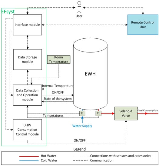
Figure 1.
EFsyst architecture.
According to Kalogirou A. S. [17], the thermal behavior of these systems can be described by:
where is the water temperature inside the tank of the EWH after a time-step , the water mass inside the tank, is the specific heat of water, is the power of the EWH, is the rate of energy removed from the storage tank, is the heat loss coefficient, and is the room temperature. Taking this into consideration, the Data Collection and Operation (DCO) module is responsible for acquiring all variables and for setting the state of the heating element at each time-step. The Data Storage (DS) module is responsible for storing all data collected over time, which support not only the real-time operation of the RCU, but also the subsequent analysis of results for assessment activities. In this study, all data storage related functionalities are ensured by the open internet of things (IoT) platform Thing Speak [18] and Wi-Fi technology is used for communication. All modules are implemented using Arduino Uno Rev3 microcontrollers [19] and ESP8266 Wi-Fi modules [20]. The Interface module is also implemented here using the Thing Speak platform and ensures the interaction of the EFsyst with the RCU and the user. The Interface module allows the access to the data stored in the DS module and is also responsible for sending the control instructions to the heating element. This interface can also provide data visualization and extraction tools to the user. The Hot Water Consumption Control (HWCC) module creates the desired profile of hot water consumption according to the instructions sent by the RCU, which are communicated through the Interface module. While maintaining the same hot water flow rate of at each time-step, a solenoid valve together with a relay are used in the implementation of the HWCC.
3. Results and Analysis
The case study considered in this paper focus a 100 L EWH, with only one heating element of 1.5 kW [21] located at the bottom of the tank, where the available energy flexibility is used to reduce electricity costs. These costs are computed according to the Portuguese tariff context, where Time-of-Use (TOU) is commonly applied. The considered prices were obtained from EDP Comercial [22] for two TOU tariffs, namely TOU-2 and TOU-3, with two and three distinct periods, respectively. Assuming a contracted power of 6.9 kVA, Table 1 shows the referred electricity tariffs (before taxes).

Table 1.
Electricity tariffs considered in this study.
The EHW under analysis is equipped with a mechanical thermostat integrated with the heating element that enables electricity supply according to the water temperature in that location. The range of operating temperatures can be manually adjusted by the user. The sensor responsible for reading the internal temperature of the tank was placed in the upper part of the equipment, where the temperature is higher and hot water is extracted when consumption occurs. In order to not impact the EWH hardware, a non-invasive implementation was adopted, placing the sensor in contact with the steel tank housing within the insulation layer. Although not proving a direct measurement of the water temperature, this sensor allows to understand temperature variations throughout the experiments according to the state of the heating element. Nevertheless, sensor T2 depicted in Figure 1 provides a direct measurement for the temperature of the consumed hot water.
Regarding the experiments carried out, three different scenarios were considered. The first one, defined as the Original Scenario (OS), refers to the normal operation of the EWH without any influence of the RCU. As presented in Section 3.1, in the OS the internal temperature varies between 47 °C and 50 °C. The second scenario, defined as T50, is characterized by the influence of the RCU, which aims to reduce electricity costs while maintaining the internal temperature between 47 °C and 50 °C. More specifically, during peak or half-peak/off-peak periods, electricity consumption is only allowed if the inside temperature is lower than 47/50 °C. The RCU also considers the temperature of the water that enters the tank (sensor T1 in Figure 1) since it was observed that the mechanical thermostat disables the energy consumption when this temperature is higher than 40 °C. Regarding the third scenario, defined as T55, it is similar to the second one but considers a maximum inside temperature of 55 °C.
In all scenarios a daily hot water consumption of 40 L was considered, which corresponds to the average daily consumption of one residential consumer in Portugal [4]. Regarding the consumption periods, it was assumed that the 40 L of hot water are consumed during a single event (no hot water consumption is verified besides this single event). All experiments were carried out at a room located in the premises of the Department of Electrical and Computer Engineering of the Faculty of Science and Technology of NOVA University of Lisbon [23].
The operation of the EWH for each scenario is illustrated in Section 3.1, while the benefits of using the available energy flexibility are presented and analyzed in Section 3.2. A 5 min time-resolution was considered by the DCO module for data acquisition, being the collected data available in [16] for the illustrative operation.
3.1. Illustrative Operation
The results presented in this section take into account the TOU-2 electricity tariff and a single hot water consumption event at 08:00. For each scenario, an experiment with a duration of two days was conducted, being the first day discarded in order to avoid undesired influences between scenarios. Figure 2 presents the room temperature during each experiment, where it can be seen that similar external conditions were registered.
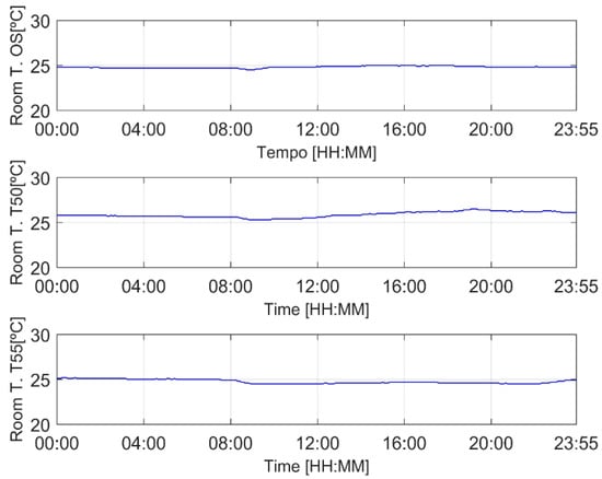
Figure 2.
Room temperature during the experiments associated to the illustrative operation.
3.1.1. Original Scenario
In the OS, the original operation of the heating element was obtained, so that it could be compared with other scenarios where the operation of the heating element is modified when using energy flexibility. The original operation is associated to a hot water temperature range at which the thermostat switches the heating element on and off according to the original values set by the manufacturer. Figure 3 shows the variation of all temperatures and the operation of the EWH on a day when consumption occurred at 08:00 for this scenario. The red background color is associated to half-peak periods, while the green one refers to off-peaks periods (this is applied throughout the remaining of the paper).
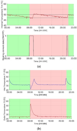
Figure 3.
Illustrative operation for the original scenario with hot water consumption at 08:00. (a) Internal temperature and heating element operation; (b) Inlet and outlet water temperature.
By analyzing the variation of the internal temperature, it was possible to determine the maximum and minimum temperature of the EWH as originally set by the manufacturer. The minimum temperature was obtained when the heating element switched from the off state (0 in Figure 3a) to the on state (1 in Figure 3a), without any external intervention, such as the consumption that occurred at 08:00. A value of 47 °C was found for this temperature, which was recorded at 21:25. Regarding the maximum temperature, a value of 50 °C was obtained at the end of heating event, which, according to Figure 2, occurred at 22:00.
In this scenario, it is possible to note that when there is consumption, the heating element is instantly turned on. This is a consequence of the location of the mechanical thermostat since it is placed near the entrance of cold water. Therefore, when consumption is registered, cold water enters the tank and the temperature at the bottom decreases significantly triggering the operation of the heating element. In Figure 3 it is also possible to observe a delay between the operation of the heating element and the consequent rise of the internal temperature due to thermal inertia.
3.1.2. T50 Scenario
In this scenario, the available energy flexibility was explored considering the same temperature range, when compared to the original operation of the EWH, in order to reduce electricity costs. The heating element was controlled according to the rules defined in the RCU, which was implemented using MATLAB (R2016a) [24] on a remote computer. For safety reasons, the mechanical thermostat was kept active to ensure that the temperature did not exceed the upper limit if an unexpected error occurred in EFsyst, which was not verified. Consequently, the control cannot be performed solely with the internal temperature due to the location of the thermostat. If only this variable was considered, when the temperature reached its maximum limit, the thermostat would mechanically open the circuit that supplies power to the heating element. Doing so would make it impossible to control the heating element while it was in the cooling period and until it reached the lower limit again. To enable full control of the heating element, both internal and inlet temperatures were used as control variables. Whenever the internal temperature is lower than the desired temperature at specific instant (47 °C and 50 °C for half-peak and off-peak periods, respectively) and the inlet temperature is lower than the limit (40 °C), the heating element is switched on. In all other cases the heating element is switched off.
The RCU reads the latest internal temperature and inlet temperature values stored in the DS module at a five minute time resolution and performs the control. Due to variations in internal temperature readings, the RCU checks if the heating element is on and reads the last temperature value. If it is off it reads the last three updated values and calculates the average, thus giving more stability to the RCU operation. Figure 4, shows the variation of all temperatures and the operation of the EWH on a day when consumption occurred at 08:00.
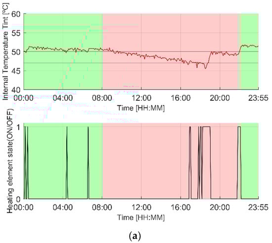
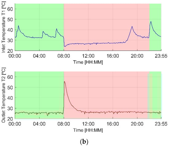
Figure 4.
Illustrative operation for scenario T50 with hot water consumption at 08:00. (a) Internal temperature and heating element operation; (b) Inlet and outlet water temperature.
When the heating element is controlled by the RCU, it is not triggered when there is water consumption at 08:00 as in the OS, and it can also be observed that the outlet temperature is higher at the instant of water consumption due to the higher internal temperature. As in the previous scenario, the electricity consumption was 2.9 kWh during the analyzed day but the associated cost was reduced by 9.4% as the consumption during half-peak period was 0.8 kWh lower.
3.1.3. T55 Scenario
The results from scenario T50 reveal that the heating element still consumes energy in the most expensive period of the TOU tariff. Therefore, in scenario T55 the energy flexibility of the EWH was increased by modifying the operating temperature range, changing the maximum temperature from 50 °C to 55 °C. The same rule-based control was used and the only difference between this scenario and scenario T50 was the higher internal temperature in the off-peak period. The inlet temperature limit was equal to that of scenario T50 in order to maintain the previous conditions and to analyze only the influence of the maximum temperature increase. This control was intended to shift the operation of the heating element only to the off-peak period. Figure 5 shows the results of this scenario with consumption at 08:00. Due to the lack of energy consumption during the half-peak period, electricity costs were reduced by 37.7% when compared to the OS.
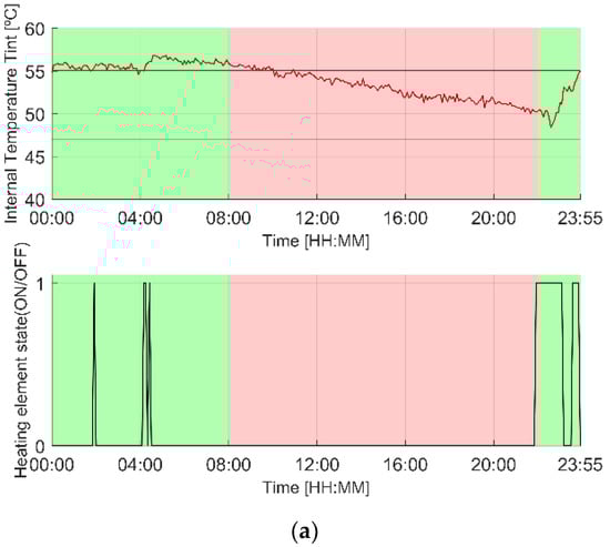
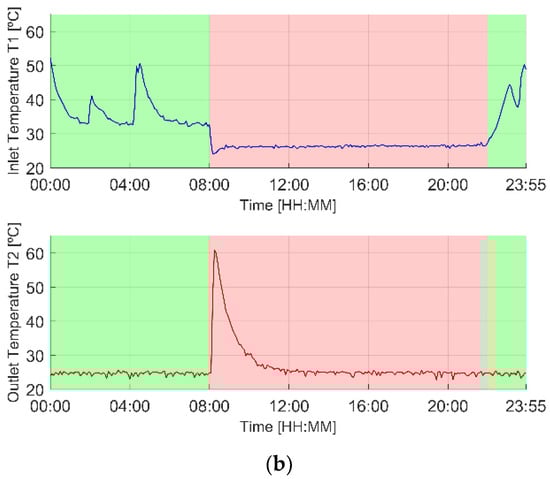
Figure 5.
Illustrative operation for scenario T55 with hot water consumption at 08:00. (a) Internal temperature and heating element operation; (b) Inlet and outlet water temperature.
3.2. Assessing the Benefits of Using Energy Flexibility
In order to better understand the benefits of using the available energy flexibility, additional experiments were conducted where the starting instant of the hot water consumption event varied throughout the day and both TOU-2 and TOU-3 were applied. Therefore, for each scenario, an experiment with a duration of six days was conducted with a single 40 L hot water consumption event per day at 00:00, 04:00, 08:00, 12:00, 16:00, and 20:00. Figure 6 and Figure 7 summarize the collected results, where the daily electricity costs for all scenarios are presented considering TOU-2 and TOU-3, respectively, together with the relative reductions achieved in scenarios T50 and T55 when compared to the original scenario.
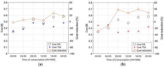
Figure 6.
Results associated to six different hot water consumption events for TOU-2. (a) Comparison between the results associated with Scenario T50 and Scenario OS; (b) Comparison between the results associated with Scenario T55 and Scenario OS.
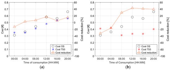
Figure 7.
Results associated to six different hot water consumption events for TOU-3. (a) Comparison between the results associated with Scenario T50 and Scenario OS; (b) Comparison between the results associated with Scenario T55 and Scenario OS.
As presented in Table 2, on average scenario T50 reduced electricity costs by 9.9% (TOU-2) and 5.7% (TOU-3) when compared to the original scenario, while scenario T55 achieved average reductions of 14.9% (TOU-2) and 17.4% (TOU-3). These reductions were achieved due to the transfer of energy consumption to the cheapest time-periods as a result of RCU control rules. The higher energy flexibility available in scenario T55 conducted to an average cost reduction of 9.3% (TOU-2) and 17.8% (TOU-3) when compared to scenario T50.
Table 2.
Summary of results.
There are, however, consumption events where the original scenario registered lower electricity costs. These events occurred at 00:00 and 04:00 and resulted from two distinct factors. The first one refers to a shift of electricity consumption to the cheapest period in the original scenario. Since in this scenario the heating element is activated as soon as there is hot water consumption, the heating events at 00:00 and 04:00 reduced electricity consumption during the most expensive periods. The second factor is related with the higher hot water temperature at 00:00 and 04:00 in scenarios T50 and T55 since in these cases the RCU aims to maintain the hot water temperature as close as possible to the upper limit. As a result, higher energy consumption is registered at these instants and higher costs are incurred despite the RCU use of energy flexibility to transfer energy consumption to the cheapest period. It is important to note that a total of 40 L was consumed, disregarding the hot water temperature. Therefore, on a real case where a mixing water tap is used, the hot water consumption flows would be lower in scenarios T50 and T55, which would result in lower energy consumption.
4. Conclusions
Existing literature shows that the development and assessment of methodologies to use energy flexibility provided by hot water heaters are mostly carried on simulation environments. These methodologies aim to achieve different objectives through the use of energy flexibility, being the most common examples related to photovoltaic and wind generation self-consumption improvement or electricity cost reduction. Due to the importance of this topic, the present paper describes a system, entitled EFsyst, aiming to support the development and assessment of the referred methodologies in real environments, where different conditioning factors should be considered. Additionally, this system allows the remote control of the electrical water heater under analysis and resource sharing.
The operation of the EFsyst is presented in this paper using a case study where the energy flexibility provided by a 100 L electric water heater (1.5 kW) is used to reduce electricity costs. Considering three different scenarios under the Portuguese electricity tariff context (one of them was design according to the original operation of the electric water heater), real data were collected during several days. The collected results show that energy flexibility can conduct to electricity cost reduction even with a simple rule based control. These savings varied from 5.7% to 17.4%, depending on the amount of energy flexibility available and the applied time-of-use tariff. Experiments considered for these results were carried during six days with a single consumption event of 40 L per day.
In order to illustrate the operation of the remote control unit, an application where the user could vary operating parameters in real time could be developed in the future. Additionally, it would be important to extend EFsyst functionalities to other heating and storage devices, or even to other type of devices, that could be controlled in order to provide energy flexibility. In terms of assessment of methodologies and systems used to explore the energy flexibility provided by EWH, the respective future experiments should consider longer periods of time (e.g., one year) in order to subject the EWH to several conditions associated to room and inlet water temperatures that can vary throughout the year. Different hot water demand profiles should also be considered in these assessment experiments.
Author Contributions
Conceptualization, R.A.L. and J.M.; literature review, T.C.P.; software, T.C.P. and R.A.L.; results validation T.C.P., R.A.L. and J.M.; writing—original draft preparation, T.C.P. and R.A.L.; writing—review and editing, T.C.P., R.A.L. and J.M. All authors have read and agreed to the published version of the manuscript.
Funding
The authors acknowledge the contribution of the Portuguese FCT-Strategic program UID/EEA/00066/2019 for providing partial financial support for this work.
Acknowledgments
The authors would like to thank the Faculty of Sciences and Technology—NOVA University of Lisbon for the institutional support and acknowledge the contribution of Fábio Januário, Fernando Coito and Luis Brito Palma during the experimental tests. The authors also acknowledge the colleagues from IEA EBC Annex67 for the valuable discussions.
Conflicts of Interest
The authors declare no conflicts of interest.
References
- European Comission. Energy Performance of Building Directive (EPBD). 2014. Available online: https://ec.europa.eu/energy/en/topics/energy-efficiency/energy-performance-of buildings/overview#content-heading-0 (accessed on 17 October 2019).
- Jensen, S.Ø.; Madsen, H.; Lopes, R. Energy Flexibility as a Key Asset in a Smart Building Future—Contribution of Annex 67 to the European Smart Building Initiatives. Position Paper of the IEA-EBC Annex 67 Energy Flexible Buildings. Available online: http://www.annex67.org/publications/position-paper/ (accessed on 10 September 2019).
- Pérez-Lombard, L.; Ortiz, J.; Pout, C. A review on buildings and energy consumption information. Energy Build. 2008, 40, 394–398. [Google Scholar] [CrossRef]
- Casaleiro, Â.; Figueiredo, R.; Neves, D.; Brito, M.C.; Silva, C.A. Optimization of Photovoltaic Self-consumption using Domestic Hot Water Systems. JSDEWES 2018, 6, 291–304. [Google Scholar] [CrossRef]
- Heleno, M.; Rua, D.; Gouveia, C.; Madureira, A.; Matos, M.A.; Lopes, J.P.; Silva, N.; Salustio, S. Optimizing PV self-consumption through electric water heater modeling and scheduling. In Proceedings of the 2015 IEEE Eindhoven PowerTech (PowerTech 2015), Eindhoven, The Netherlands, 29 June–2 July 2015. [Google Scholar] [CrossRef]
- Fitzgerald, N.; Foley, A.M.; McKeogh, E. Integrating wind power using intelligent electric water heating. Energy 2012, 48, 135–143. [Google Scholar] [CrossRef]
- Pourmousavi, S.A.; Patrick, S.N.; Nehrir, M.H. Real-Time Demand Response through Aggregate Electric Water Heaters for Load Shifting and Balancing Wind Generation. IEEE Trans. Smart Grid 2014, 5, 769–778. [Google Scholar] [CrossRef]
- Du, P.; Lu, N. Appliance Commitment for Household Load Scheduling. IEEE Trans. Smart Grid 2011, 2, 411–419. [Google Scholar] [CrossRef]
- Al-Jabery, K.; Xu, Z.; Yu, W.; Wunsch, D.C.; Xiong, J.; Shi, Y. Demand-Side Management of Domestic Electric Water Heaters Using Approximate Dynamic Programming. IEEE Trans. Comput. Des. Integr. Circuits Syst. 2017, 36, 775–788. [Google Scholar] [CrossRef]
- Kepplinger, P.; Huber, G.; Petrasch, J. Autonomous optimal control for demand side management with resistive domestic hot water heaters using linear optimization. Energy Build. 2015, 100, 50–55. [Google Scholar] [CrossRef]
- Kapsalis, V.; Safouri, G.; Hadellis, L. Cost/comfort-oriented optimization algorithm for operation scheduling of electric water heaters under dynamic pricing. J. Clean. Prod. 2018, 198, 1053–1065. [Google Scholar] [CrossRef]
- Lin, B.; Li, S.; Xiao, Y. Optimal and learning-based demand response mechanism for electric water heater system. Energies 2017, 10, 1722. [Google Scholar] [CrossRef]
- Wu, Q.; Wang, L.; Li, B. An optimized demand response strategy for electric water heaters and the associated impact on power system operational reliability. In Proceedings of the 2017 International Smart Cities Conference (ISC2), Wuxi, China, 14–17 September 2017. [Google Scholar] [CrossRef]
- Ruelens, F.; Claessens, B.J.; Quaiyum, S.; de Schutter, B.; Babuška, R.; Belmans, R. Reinforcement Learning Applied to an Electric Water Heater: From Theory to Practice. IEEE Trans. Smart Grid 2018, 9, 3792–3800. [Google Scholar] [CrossRef]
- Shah, J.J.; Nielsen, M.C.; Shaffer, T.S.; Fittro, R.L. Cost-Optimal Consumption-Aware Electric Water Heating Via Thermal Storage under Time-of-Use Pricing. IEEE Trans. Smart Grid 2016, 7, 592–599. [Google Scholar] [CrossRef]
- EFsyst Data. Available online: https://github.com/taapereira/EFsystdata (accessed on 6 November 2019).
- Kalogirou, S.A. Solar Water-Heating Systems. In Solar Energy Engineering Processes and Systems, 2nd ed.; Academic Press: Cambridge, MA, USA, 2014; pp. 257–321. ISBN 978-0-12-397270-5. [Google Scholar]
- ThingSpeak. Available online: https://thingspeak.com/ (accessed on 11 August 2019).
- Arduino Uno Rev 3. Available online: https://store.arduino.cc/arduino-uno-rev3 (accessed on 11 August 2019).
- ESP8266. Available online: https://www.espressif.com/en/products/hardware/esp8266ex/overview (accessed on 11 August 2019).
- Electric Water Heater Delta V 100L. Available online: https://www.leroymerlin.pt/Produtos/Canalizacao/Termoacumuladores/WPR_REF_14429254 (accessed on 14 March 2019).
- EDP Comercial. Available online: https://www.edp.pt/particulares/energia/tarifarios/ (accessed on 20 August 2019).
- Departamento de Engenharia Eletrotécnica e de Computadores da Faculdade de Ciências e Tecnologias. Universidade Nova de Lisboa. Available online: https://www.dee.fct.unl.pt/ (accessed on 11 September 2019).
- MATLAB. Available online: https://www.mathworks.com/products/matlab.html (accessed on 11 September 2019).


© 2019 by the authors. Licensee MDPI, Basel, Switzerland. This article is an open access article distributed under the terms and conditions of the Creative Commons Attribution (CC BY) license (http://creativecommons.org/licenses/by/4.0/).