Abstract
The ongoing upsurge of deep learning and artificial intelligence methodologies manifest incredible accomplishment in a broad scope of assessing issues in different industries, including the energy sector. In this article, we have presented a hybrid energy forecasting model based on machine learning techniques. It is based on the three machine learning algorithms: extreme gradient boosting, categorical boosting, and random forest method. Usually, machine learning algorithms focus on fine-tuning the hyperparameters, but our proposed hybrid algorithm focuses on the preprocessing using feature engineering to improve forecasting. We also focus on the way to impute a significant data gap and its effect on predicting. The forecasting exactness of the proposed model is evaluated using the regression score, and it depicts that the proposed model, with an R-squared of 0.9212, is more accurate than existing models. For the testing purpose of the proposed energy consumption forecasting model, we have used the actual dataset of South Korea’s hourly energy consumption. The proposed model can be used for any other dataset as well. This research result will provide a scientific premise for the strategy modification of energy supply and demand.
1. Introduction
The world is witnessing a rapid shift toward renewable energy sources. Amidst the expanding market for electricity with time, it is alluring to make policies accordingly. Subsequently, it is imperative to estimate power load demand precisely. Forecasting is an active area of research in both government and private sectors. Forecasting is the most reliable approach to design and plan future policies. Renewable energy farms such as wind farms, solar energy farms, and wave power farms need accurate forecasting. Such predictions are related to the operating preferences of power system management, for example, the opening and closing of traditional power generation equipment, excessive power generation provided through the energy market, etc. [1]. Load forecasting includes accurately predicting each size and geographic location within a specific interval of the planned area. The basic type of prediction used is usually the total system load per hour. However, load forecasting also involves forecasting hourly, daily, weekly, and monthly load and peak load values. From the administrative point of view, managing the power supply and electricity cost typically includes from a few days to three-month forecasts. In many cases, particularly in estimates of the price of electricity, the current valuation does not depend on the expectations of actual points but rather on the allocation of power demand at certain times in the future.
The efficient control and planning of electrical systems require power demand forecasting. In the early energy prediction, statistical strategies with general or decisive heuristic information were applied. Energy consumption is an essential basis for determining energy policy and programming, especially in developing countries. Accurate energy consumption forecasting can provide compelling reference records for leaders and regulators to achieve sustainable energy development. Increasing greenhouse gas levels is also a significant concern that urges world leaders to make policies for electricity generation [2]. Under the pressure of environmental pollution and the power crisis, various international sites are devoted to developing sustainable electrical sources, such as hydro, wind, solar, geothermal, and bioenergy. A viable electricity strategy plays a critical role in energy generation [3]. The consumption of energy includes many factors. It contains specific patterns, daily, weekly, weekly periodic cycles, and specific seasonal characteristics of other important dates. The changes in consumer demand can similarly affect seasonality and schedule effects.
Time series data is used to forecast the future demand and consumption of electricity. Different machine learning (ML) algorithms are used to predict time series data. Missing values cause depreciation in the forecast performance of energy consumption, and they must be imputed by filling in other values. In these circumstances, we can neglect when the missing data ratio in the total data is less than 1%. If the missing rate is between 1% and 5%, it is considered a manageable or flexible sample data. On the other hand, missing data rates >5% of the complete data demand proper resolutions. Moreover, missing data rates of >15% significantly unfavorably influence the forecast model [4].
XGBoost belongs to a family of boosting algorithms and it uses the gradient boosting framework at its core. It is a smooth, distributed gradient boosting library. The speed and execution have made XGBoost especially successful. It is comparatively faster than other group classifiers [5]. XGBoost can bridle the intensity of multicore computers, and it is attainable to execute on large datasets. It has indicated better execution on different machine learning benchmark datasets. XGBoost has parameters for crossvalidation, regularization, user-defined objective functions, missing values, tree parameters, and so on. Random forest is another ML model that is often used to predict large amounts of data. Random forest usually generates a very accurate classifier. Random forest is an integrated learning method that can involve the prediction of multiple decision trees [6]. The basic principle involved in the random forest is called bagging, where a sample is randomly selected from the training set and fitted to the regression tree. A bootstrap sample is drawn, and that sample can be picked with substitution. In such a scenario, one similar sample can appear multiple times. A CatBoost is an open-source machine learning algorithm. It is based on gradient boosting over decision trees. An organization called Yandex created CatBoost. It is the successor of the MatrixNet algorithm that was broadly utilized inside the organization for ranking assignments, anticipating, and making recommendations. It is widespread and can be applied across a wide variety of fields and situations [7]. The early stopping characteristic of the CatBoost library additionally forestalls overfitting by ending the training and contracting the model if no improvement for the loss function is made in the testing datasets. The hybrid approach has come up as a new technique for the energy consumption forecasting domain. Compared to the practice of a single system of forecasting, the combination of forecasting techniques can be implemented for more accurate outcomes. Within the literature, we found two sorts of hybrid methods: a combination between a traditional model and artificial intelligence (AI) method and a hybrid between two AI methods. Due to the ability of the AI strategies to achieve higher performance than the mixture of one conventional system and one AI technique, the blending of two AI approaches is exceptional [8].
The South Korean government has proceeded with the renewable energy advertising coverage to make Jeju island a carbon-less peninsula by the year 2030 [9]. The policy has been strictly executed, particularly regarding state and local government workplaces. Following this policy, the South Korean authorities started the renewable energy portfolio standard (RPS) and feed-in-tariff (FIT) programs, which require energy companies to present a base proportion of their power request employing suitable renewable energy assets. Furthermore, the legislature applied incredible exertion to introduce and promote an economical energy system by using geothermal heat, solar electricity, wind electricity, and tidal power. Besides, the South Korean government has designated that both public and private sectors ought to efficaciously participate in the flow of renewable energy technology facilities and highlight satisfying the residents’ electricity needs [10].
We proposed an energy forecasting system using the state-of-the-art machine learning algorithms. We have performed our simulations for prediction models on the actual dataset of energy consumption of South Korea. A hybrid supervised machine learning technique is proposed. We have used three states-of-the-art bagging and boosting algorithms. XGBoost, CatBoost, and random forest models learn and train based on the errors of the previous boosting algorithm. They give better performance as compared to these individual models. There are different techniques available to fill the null values, but these imputation techniques do not work when there is a large data gap. We have proposed a method to fill the large gap and then train our proposed model based on the new dataset. The significant contributions of this article are
- Presenting a hybrid ML algorithm for energy prediction.
- Data imputation technique for the large gap in the dataset.
- Comparing the forecasting results with data imputation and without data imputation.
- Comparing the forecasting results with existing ML models.
The rest of the paper is organized as follows: In Section 2, related publications, articles, and materials are examined and discussed. In Section 3, the energy management system of the Korea power exchange is discussed. In Section 4, the process flow of our energy forecasting scheme and data imputation is explained. We also analyze our dataset in this section. In Section 5, we describe the proposed hybrid ensmebled model, objective function, architecture, and its use for data imputation. Exploratory data analysis, trends of the data, and fine-tuning for forecasting are explained in Section 6. In Section 7, the performance results of the proposed model are provided with training data. An analysis of all data generation methods is also discussed. We also compare our results with bagging boosting, statistical, and neural network-based models. We conclude this work and provide instructions for future research in Section 8.
2. Related Works
Artificial intelligence-based frameworks such as neural networks (NN), machine learning, and big data are changing the dynamics of forecasting. The advancements in these fields are just remarkable and they are helping the policymakers to design policies based on trusted predictions. Table 1 demonstrates some other ML-based hybrid techniques used in forecasting. Lee, S. et al. [11] proposed an algorithm that was developed and prepared using training data created by Levenberg–Marquardt propagation to perform power prediction performance of commercial structures. The proposed scheme gives better results as compared to medium-impact value strategies through experiments. The results show that using energy consumption models in critical stages and using advanced and compelling examples for data generation can achieve acceptable implementation. Kim, M. et al. [12] proposed a model for energy consumption prediction in residential buildings. Looking at the consequences of the regression analysis, the input factors used to train the artificial neural network (ANN) model for each period are selected, and an energy consumption prediction model is applied based on actual consumption. First, the investigation depends on the actual energy consumption of the Korean housing structure. Besides, the components are identified by coordinating the physical and customer data of the building and reproducing the collective impact. Finally, the energy forecasting model is implemented by dividing the energy consumption rate into four seasons and identifying attractive components for each season.

Table 1.
ML-based hybrid models for forecasting.
In an article by Ahmed et al. [22], prediction of hourly solar radiation is presented for New Zealand. The potential to offer twenty-four hour forecasts was evaluated, making use of various strategies, mainly consolidating auto regressive recurrent neural networks. Hourly time series had been applied for training and testing the forecasting techniques. Root mean square error (RMSE) was adopted to compare nonlinear auto-regressive exogenous (NARX), multilayer perceptron (MLP), auto-regressive moving average (ARMA) , and persistence techniques. According to the results, the method exhibited an accuracy more distinguished than that of the ARMA, MLP, and persistence methods. NARX method had the lowest value of RMSE. In the research by Chahkoutahi et al. [23], a seasonal optimum hybrid version to forecast the energy load is introduced. The main motivation for the practice of this model was to utilize different models’ benefits for modeling complex methods. A direct optimum parallel hybrid model (DOPH) was presented using a multilayer perceptron neural network, seasonal autoregressive integrated moving average (SARIMA), and adaptive network-based fuzzy inference system (ANFIS) to forecast the energy load. The validation of the exhibited model suggests that it was much more reliable than its components. RMSE was used to compare the output of every technique with target values. The recommended DOPH method was compared against MLP, SARIMA, ANFIS, differential evolution (DE) based, and genetic algorithm (GA) based models. According to conclusions, the suggested approach could enhance the forecast tendency as compared with the MLP, SARIMA, ANFIS, GA, and DE based techniques.
Various electricity systems efficaciously utilize decision tree techniques. These approaches are used to approximate discrete-valued objective functions that a decision tree represents the learned function. These are amongst the various practical inductive reasoning algorithms. The forecasting of protein-ligand binding is an essential factor in the designing phase of drugs. Protein-ligand binding forecasting computational techniques are modest and quick test strategies. Zhao, Z. [24] proposes another computational model, which incorporates the XGBoost and synthetic minority over-sampling technique. Tropical cyclones are a significant reason for an enormous death toll and property. Although the capacity of numerical climate expectation models to estimate and track tropical cyclones has significantly improved but anticipated the power of a tropical storm is still exceptionally troublesome, in this manner, the increment of prediction accuracy of tropical cyclone forecast is essential. Jin, Q. et al. [25] utilizes the XGBoost model to estimate tropical cyclone in coastal urban areas of China. They built up a progression of indicators using the best track tropical cyclone dataset to foresee the 6, 12, 18, and 24 h forces of tropical cyclone for the period 1979–2017 under six situations utilizing the XGBoost model.
Illegal insider trading distinguishing proof presents a problematic assignment as trading activities within the trade have caused real damage to the confidence of financial experts and the economic improvement of the stock market [26] proposes another validation method, which can format XGBoost and a non-dominant sorting genetic algorithm (NSGA) to oversee domestic trade. Initially, identify the local trade cases that occur in the Chinese stock market, and identify and obtain their appropriate markers. By then, the proposed strategy had trained the XGBoost model and used NSGA to use various objective functions to improve XGBoost parameters. Finally, use the XGBoost advanced settings to mark test samples. Both distinguish the accuracy and efficiency of the evidence through evidence from different periods. Lahouar, A. et al. [27] recommend a short-range prediction system for random forest technology. The system is designed to provide forecasts one day in advance for the conditions pertaining to Tunisian electrical installations, such as small areas, warm weather, disorganized energy, and backups. The main contribution of this article is to explain the possibility of adapting to a random forest when it relates to feature selection to manage any electricity profile, especially to adapt to complex customer behavior. The proposed method is highly accurate and effective in all seasons and dates specified. Zhang et al. [28] practiced the CatBoost algorithm for feature selection in estimating electricity costs. They introduced a new two-layer feature selection strategy based on the CatBoost algorithm to overcome the trouble that traditional gradient enhancement methods cannot effectively solve specific attributes. Deng and colleagues [29] suggest a hybrid system to predict short-term pregnancy enhanced by a switching algorithm that improves delayed particle swarm optimization algorithms. In this study, a technique based on empirical mode decomposition (EMD), switching delayed particle swarm optimization (SDPSO), and extreme learning machine(ELM) were introduced. The first step is to analyze the history of the electricity consumption database and to calculate the intrinsic mode entropy (IME) value. The intrinsic mode functions are divided into three categories. ELM is then applied to predict these three categories. Finally, the final prediction value is obtained by aggregating the prediction results. Fu, G. et al. [30] presented an ensemble technique for prediction of the cooling load of the air-conditioning system. The proposed technology was used for deterministic prediction of the cooling capacity beside tremendous accuracy. This technique utilized a deep belief network (DBN) and ensemble empirical mode decomposition (EEMD) methods. They decompose the actual cooling load data series into many components. The influence of uncertainties is mitigated by using the ensemble method.
Some islands in South Korea have introduced a small independent grid system that can operate freely without grid connection and replace diesel generators with non-renewable energy. Several research articles analyze the productivity of these systems. For example, Yoo, K. et al. [31] tried the economic feasibility of an independent power generation framework on Ulleung Island, one of the far East Islands in South Korea. They designed an improved design to provide renewable power generation. Vehicles used in daily life transportation system is a significant source of global warming, CO2 emissions, and consumption of petroleum product. The presentation of new methods for transportation is a global issue. The improvement and appropriation of electric vehicles are an answer to this issue. Bai, K. et al. [32], taking into account Hongdao Island, South Korea as an example, has proposed a hybrid wind energy framework, which consists of two wind turbine models and an independent diesel generator. Their study shows that energy expenditures account for 84% of the renewable energy share. Jeju’s local government is especially active in implementing renewable energy transfer strategies and assisting it in supply. Japa Island is a small island in southern Jeju. In the first stage of implementing the local plan, because Jeju has just made Gapa a carbon-free island. The island’s diesel generators are complemented by new sustainable energy sources, especially wind and solar. Jeju keeps on executing its carbon-free arrangements. Jeju local government proposes to accomplish more than half the percentage of renewable sources with smart-grid systems, and wind turbines [33].
3. Energy Management System
For the testing purpose of the proposed energy consumption forecasting model, we have used the actual dataset of South Korea’s hourly energy consumption. We obtained the data from the Korea power exchange (KPE). This exchange is responsible for the power trading process in South Korea. It has an energy management system (EMS) which works based on energy demand forecasting. Figure 1 shows the power trading system configuration for the EMS of Korea power exchange.
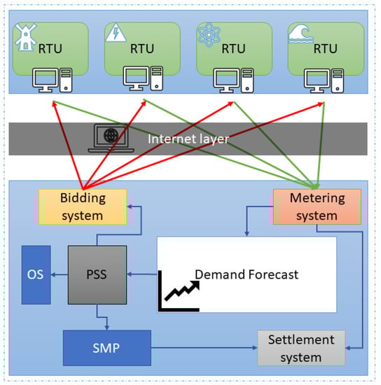
Figure 1.
Energy trading system configuration.
KPE have different remote terminal units (RTU) for energy generation, which send the data to the central metering system using internet protocols. They post the available capacity results over the internet for where RTUs can do biding. The effects of demand forecasting are essential for price-setting schedule (PSS) and operational schedule(OS). With the help of PSS, they also adjust the system marginal price, which ultimately helps in the settlement system and other payment systems.
4. ML based Energy Load Forecasting
ML is helping many fields of data science, including energy data. A typical machine learning pipeline is shown in Figure 2. It starts with data acquisition for prediction purposes. Preprocessing of data includes, fill missing values, removing outliers, and exploratory data analysis. The smooth data is provided to the ML model, and then at the end, that model is evaluated on the test data. For the testing purpose, we have used the real data of the energy consumption of South Korea. The Republic of Korea covers an area of 100,210 km2 and a populace of over 51 million individuals. South Korea is going to change over the entirety of its vehicles into electricity as a stage towards the carbon-free island. Jeju Island intends to become carbon-free and completely economical by utilizing sustainable power sources. Solar panels, geothermal vitality, and wind turbines are contributing their jobs in the generation of efficient green energy [33]. To make the policies in this regard energy forecasting is of great importance. We got the data in XML format, so we converted that into CSV format for further use. The data is split into two parts: training data and testing data. After preprocessing data is provided to the ML model where it trains, and then it is evaluated on the testing data.
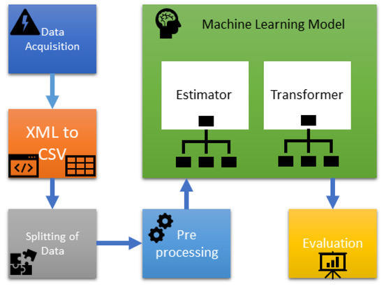
Figure 2.
Process flow of energy forecasting.
4.1. Data Imputation
Missing data may affect the performance of the prediction model. It affects the precision and also leads to bias estimation result of the analysis. Missing data can be present in the form of 0, −1, or NaN. The method of replacing missing data with substituted values is called imputation. While choosing the right approach for imputation first, we have to analyze the mechanism of missingness to see if it is missing at random or not. There are three common patterns of missing data.
- Missing completely at random (MCAR) means that the lacking information is unbiased on any variable found in the information set.
- Missing at random (MAR) approach that the missing statistics may rely upon variables located in the facts set, but no longer on the missing values themselves.
- Not missing at random (NMAR) approach that the lacking facts relies upon on the missing values themselves, and no longer on any other located variable. There are three conventional approaches to fill the missing records.
We examine the patterns of missing data according to our dataset.
4.1.1. Drop Missing Values
The fastest and easiest way to handle missing value is to drop it. However, it will reduce the quality of the forecasting model as it reduces the sample size. This technique can be applied to the MCAR pattern of missing data. It will delete all records where any variable is null or missing. In our real dataset. Table 2 presents the summary of year-wise data. According to that, we have 21.26% of missing data, so we can not drop such a large amount of dataset.
Table 2.
Year wise data summary.
4.1.2. Fill Missing Values with Test Statistic
One of the conventional methods for data imputation is the use of statistical purposes, such as mean, median, or mode of a specific feature. Statistical methods are the right approach for a small dataset, and they can prevent the loss of rows and columns. But it adds variance and bias. This technique can be applied to the MAR pattern of missing data. Figure 3 shows the Comparison of data before and after interpolation. Figure 3a is the representation of actual data set and Figure 3b shows the data set after interpolation. The X-axis depicts the date in years of recording the data, and Y-axis shows the energy load in MW. When we used the linear interpolation method to our dataset, it imputes the data, but the values are less than 60,000 and more significant than 5000, which is quite different from the general trend. That’s why we can’t use this method on the dataset with a large gap.
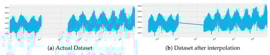
Figure 3.
Comparison of data before and after interpolation.
4.1.3. Fill with A Machine Learning Algorithm
The most effective and best way to handle missing values in a large amount is by using the predictive models. In this method, we separate the null values and train the model on the remaining values. Then use that model to predict the missing values. It results in the estimation of unbiased model parameters.
5. Proposed Hybrid Ensemble Model
Different ML models have pros and cons. We have proposed a hybrid model that uses different boosting and bagging based models to generate various base classifiers. A new classifier is derived using Equation (1). which performs better than any constituent classifier. The key objective of the proposed method is to reduce bias and variance. Figure 4 depicts the architecture of our proposed imputation and forecasting model. A dataset with a large data gap is imputed using the hybrid model. The proposed model is applied to the dataset before and after a large gap. Then take the mean of predictions from both models. The final dataset is again given to the model and validated from test data. In the results section, we have provided a comparison of forecasting results with imputation and without imputation. A complete training dataset is given to the hybrid model and trained. Every model within the box uses a different algorithm. The predictions made from these N models are used as predictors for the final model. The variables thus collectively formed are used to predict the final classification with more accuracy than each base model using Equation (2) where are base classifiers, are weights, n is the number of models, and is our final classifier with a weighted average.
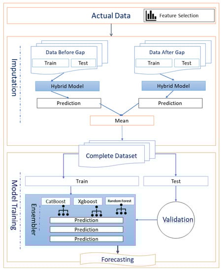
Figure 4.
Architecture of proposed imputation and forecasting model.
In this technique, the dataset is directly divided into training and validation instead of k-fold validation. Figure 5 shows the concept diagram of classifiers. The output of the Level 0 classifiers is used as training data for the final classifier at Level 1.
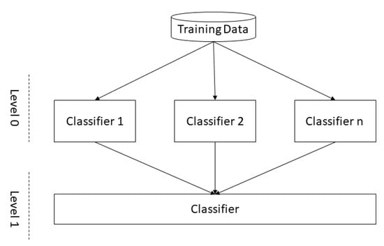
Figure 5.
Concept diagram of classifiers.
5.1. Hybrid Objective Function
The objective function of the hybrid model begins with the training of different algorithms. It requires continuous inputs and the power load output, and then the average output of these models trained with hybrid functions defined in the Equation (3).
In this objective function, j is the index for each algorithm, and denotes the weight of of each objective function. For our hybrid model, we choose three state of the art ML algorithms, which include XGBoost, CatBoost, and random forest. We train these three models separately as well for the comparison with the hybrid model.
5.1.1. Extreme Gradient Boosting (XGBoost)
Extreme gradient boosting (XGBoost) is a scalable ML method that was introduced by Chen and Guestrin [34]. It follows the boosting principal. Boosting is used to create an active learner from weak learners. It learns sequentially by fitting the current regression tree to the mistakes from the last tree. This newly generated tree is then introduced into the adapted version to update the error. It also constructs the new regression tree to maximize correlated to negative of the gradient loss function [35]. Gradient gradients can learn directly from residual errors or mistake instead of updating the recorded point weights. Gradient boosting starts training the selection tree and then follows the selection tree; only an improved tree can predict and calculate the rest of the decision tree. Save these residual errors as a new y. Repeat this process until it reached the number of trees that are set up for optimal solutions. Then it makes the final prediction.
5.1.2. CatBoost
CatBoost is a gradient boosting library that can manage categorical data. This model configures the connected values, then calculates the pseudo residual and measures the appropriate base learner for the pseudo residual. Then, it calculates the multiplier and replaces the pattern [36]. CatBoost does not use binary classification. Alternatively, it can perform any substitution on the data set. A category value similar to the previous value in the replacement is used to calculate a typical loss. This method is used to search for expression features. The Equation (4) is used to convert these categorical features into numerical features. Where is the averages target and to calculate this we used in class counter , starting values for numerator (P) and total counter (Ct).
5.1.3. Random Forest
Random decision forests is an ensemble learning approach for classification, regression, and other obligations that perform by constructing several decision trees [37]. Unlike the metadata estimator, random forest randomly identifies a fixed set of functions that can be used to determine the exact split on each node in the selection tree. The command starts with the boot mode, which is a random subset of M in the x training set, and this process is called bootstrapping. Then the tree grows from the bootstrap sample and randomly selects the variables from x. At each node in the decision tree, only a set of random features is considered to determine the best split. Optimal separation is used to divide nodes and tree growth without pruning. It predicts the records to be created in each tree’s test set, and eventually performs regression using Equation (5). Calculate the final forecast by comparing the estimated values of all decision trees.
5.2. Proposed Imputation Method
In our dataset, we observed the NMAR pattern of missing data. The gap between data is huge, so we made a hybrid model on the bases of boosting algorithms. First of all, we divide our non-missing dataset into two subsets. one is before gap, represented in Figure 6a, and other is after gap represented in Figure 6b. Then we apply a hybrid model on each dataset and take their predictions on gap values. In the end, we take the mean of both models. Then we fill our gap using the output of the hybrid imputation model.
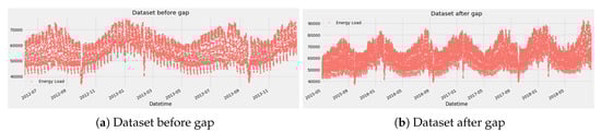
Figure 6.
Division of data into two parts.
In Algorithm 1 we have presented the pseudocode for data imputation. We divide the dataset into three subsets, where is missing data, is data before the gap, and is data after the difference. We apply the hybrid model on both and separately. Then take the mean of both predictions using Equation (6).
where is the output of imputation function. n is the number of observations and is prediction for . Then we concatenate our three subsets , and into one. Figure 7 shows the complete data set after applying the imputation method.
| Algorithm 1 Pseudocode for data imputation. |
|
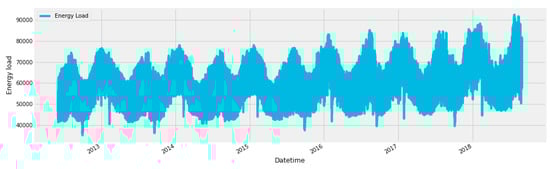
Figure 7.
Full dataset after imputation.
6. Forecasting
We have used the complete dataset for the forecasting of energy load. We also compare the results of our proposed model with the imputed and missing data sets. For the prediction, we first divide data into test and train data sets. Then tune the parameters for the training of our model, and in the end, we analyze our model based on test data.
6.1. Exploratory Data Analysis
We collected the recent real energy consumption data of South Korea from year mid of 2012 to the middle of 2018. This data is recorded on an hourly bases. So we got 24 entries per day of energy load. To better understand the patterns of our data, we perform Exploratory data analysis (EDA). It serves as the foundation stone of our machine learning algorithm. It also helps to analyze the missing value and there impact on forecasting. We analyze the data set by dividing it into different sections. Figure 8a shows the energy load per hour. Figure 8b depicts the power usage per day of the week, and Figure 8c explains the power usage per week of the year.
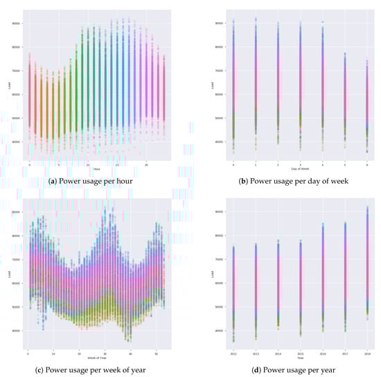
Figure 8.
Trends of power usage.
We took the median of hourly demand per day, represent it in graphical form in Figure 9. There are four quarters in a year and to analyze the distribution over Seasonality we plot boxplot shown in Figure 10.
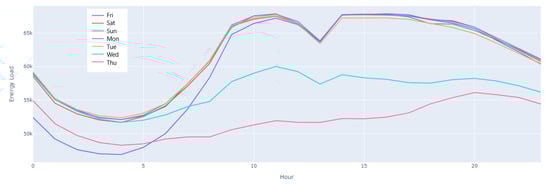
Figure 9.
Median hourly power demand per weekday.
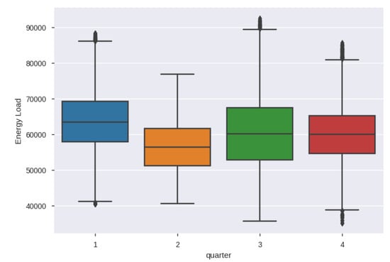
Figure 10.
Seasonality analysis: Distribution over quaters.
6.2. Training
In general, the large number of estimators and small learning rates produce correct models. However, it takes the model delayed time to train because it does more significant repetitions by the round. We provide learning rate as 0.1 and estimators as 1000. We give early stopping rounds as 50, so it keeps on training until it hasn’t improved in 50 rounds. We get the 0.81% Mean Absolute Percentage Error. We got the absolute error from the range 6.40% to 0.23%.
6.3. Train-and-Test Split
We divided our final data into two parts, test and train. As shown in Figure 11, the data after 2017 is used as our validation set. In the training data starting from 2 June 2012 to 1 January 2017, every day consists of 24 h. Energy load reading was saved on hourly bases, so we get the 24 entries for each day. While training a model for energy forecasting, the complete data set can be used as training data. But here we want data for testing and evaluation of our proposed model as well. For this purpose, we have split a large amount of data for testing purposes.
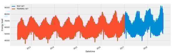
Figure 11.
Data split into test and train data.
Pearson is most appropriate correlation for measurements taken from an interval scale. Linear relationship among two continuous variables ca be evaluated by pearson correlation [38]. We made the Pearson correlation graph of Train data shows in Figure 12. It shows that feature is highly correlated with (). Whereas day of year is highly correlated with () and week of year is highly correlated with day of year ().
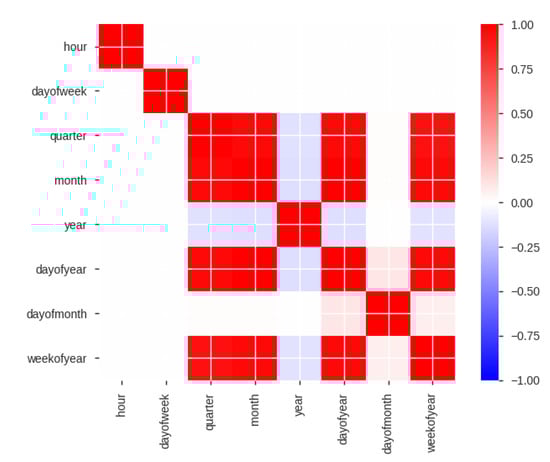
Figure 12.
correlation graph of train data.
7. Experimental Results and Discussion
This section presents the results of our simulation and already existed algorithms. We performed simulation and experiments on python tensor flow version 1.15.0 on the core i-7 processor with 16 GB RAM. GPU used for operations has NVIDIA GeForce RTX 270 with the memory of 16 GB. we also import different libraries and packages of python Table 3 include some relevant Packages and their versions used for simulations. NumPy(1.17.5, NumPy Developers) is used for high-level math calculations, and to make graphs, we used the plotly package. The dataset contains 54,730 unique rows. Every record depicts the energy load of one hour of South Korea. The experimental results were compared with those of XGBoost, CatBoost, and random forest individually.
Table 3.
Packages used for simulation.
7.1. Feature Importance Analysis
Feature scaling is essential for regressions models. A straightforward way of doing this entails counting the wide variety of times each function is split on throughout all boosting trees. After which visualizing the result as a bar graph, with the tasks ordered in line with how commonly they appear. We have used three base models, and every model generates different feature importance score. The three dimensions of features importance are frequency, gain, and cover. Figure 13 shows the graphs of the feature importance cover and gain.
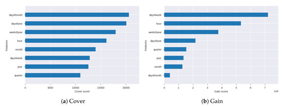
Figure 13.
Feature importance score of gain and cover.
Coverage is the number of times an item is used to split data across all trees, and this number outweighs the number of training data points passed by these sections. The scale indicates the relative number of observations associated with this function. Figure 13a depicts the bar graph for cover score of all the features. Gain is the average reduction in training loss when using the specific feature. The gain gives the relative contribution of the corresponding feature in the model, which is calculated by the contribution of each feature of each tree in the model. Compared to other attributes, a higher value for this measurement indicates that it is important to generate predictions. Figure 13b shows the bar graph for gain score of all the features. Frequency or weight is the percentage, and sometimes represents the percentage of a specific function in the model tree. The weight percentage of one feature accounts for the weight of all functions to calculate the frequency.
Figure 14 shows the graphs of the feature importance frequency of each model. CatBoost calculates the importance of features according to the impact of feature value change on average prediction changes. If the value is high, it’s mean it will have more impact on the change of prediction value. In CatBoost feature is the most important feature as shown in Figure 14a. Random forest calculates feature importance as the decrement in node impurity weighted by the probability of reaching that node. Feature has the highest value as shown in Figure 14b in random forest. In XGBoost, it is relatively straightforward to retrieve the importance score for every feature. Significance is determined for a single choice tree by the sum that each trait split point improves the exhibition measure, weighted by the number of observations of every node. In our dataset, the feature has the very best importance score, according to XGBoost, as shown in Figure 14c.
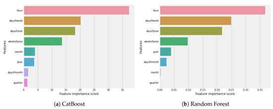
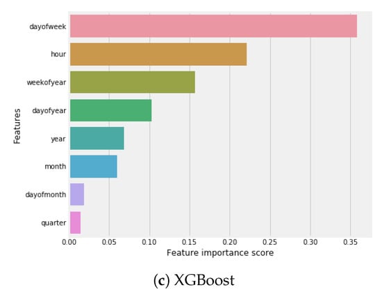
Figure 14.
Feature importance with ML models.
7.2. Forecasting Results
We applied the trained model on test data and visualized different predictions of the proposed model. Figure 15 shows the visual representation of actual and predicted values of overall test data.
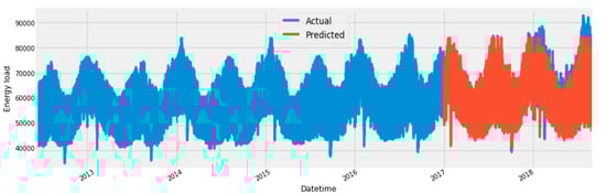
Figure 15.
Overall prediction using hybrid Model.
To make the visualization more clear we plot graphs of a single day and a single month from the test data as well. Figure 16 represents the one day prediction of best predicted day. we observed the absolute error as 0.23% at this point.
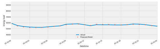
Figure 16.
Best predicted day.
We selected a random month to plot the actual and predicted value from test data. Figure 17 represents the prediction of June 2018.
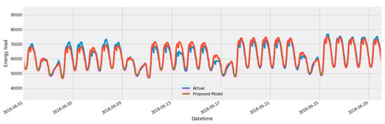
Figure 17.
Forecast for the month of June.
The predicted vs. observed scattered points are distributed around the y = x reference line, and the density of points is closer to the reference line. Figure 18 exhibits a reasonable linear regression through proposed model. a blue line on top of the scatter plot represents the resulting inputs and predicted y-values for the dataset. This graph shows that the model has learned the underlying relationship in the dataset.
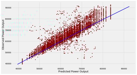
Figure 18.
Scatter plot of predication v.s. test data.
7.3. Boosting Trees
Boosting trees plots provide insight into how the model arrived at its final decisions and what splits it made to arrive at those decisions. Figure 19 shows one such tree obtained from XGBoost model.
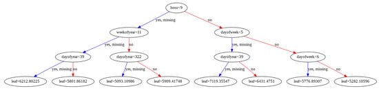
Figure 19.
Boosting Tree.
7.4. Model Goodness Inspection
In this part, the forecast outcomes acquired by the hybrid model is assessed by two statistical signs, to higher take a look at the goodness of fit. These indicators are mean absolute error (MAE) and regression score . Equation (7) is used to calculate MAE [39].
7.4.1. Mean Absolute Error
Figure 20 the mean absolute error graph of whole data set. In the worst scenario we got the 6.40% absolute error and in the best scenario we got 0.23% absolute error.
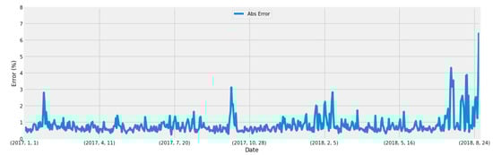
Figure 20.
Ensembled method error graph.
7.4.2. Regression Score
To further compare the performance of different models, the regression score is used [40]. This score is calculated by using Equation (8). The R-squared is a relative measure of the appropriate fitting of the regression model. R-squared has the advantage of its intuitive scale: it varies from zero to one. Zero indicates that the proposed model does not improve on the average model, while the one shows an ideal prediction. The improvement of the regression model leads to a relative increase in R-squared.
Table 4 shows regression score of our proposed models and comparison with ensemble models, extreme gradient boost, CatBoost, and random forest models. We have also compared our proposed model with a statistical model ARIMA (0.10.2, statsmodels) and neural network-based models GRU (2.3.1, Keras) and LSTM (2.3.1, Keras). The comparison shows that our proposed model performs well as compared to existing statistical and ensemble models. Table 4 shows regression score of our proposed models and comparison with ensemble models, extreme gradient boost, CatBoost, and random forest models. We have also compared our proposed model with a statistical model ARIMA, and neural network-based models GRU and LSTM. The comparison shows that our proposed model performs well as compared to existing statistical and ensemble models.
Table 4.
Comparison of overall regression score with existing models.
7.4.3. Comparison with Existing Models
In the comparison section, we choose the state of the art models for the comparison with the proposed model. We also compared our proposed model with and without imputation.
In Figure 21, we have compared our proposed model with two different data sets. One is the original data set, which has a large data gap, and the other is an imputed dataset. Figure 22, shows comparison of our proposed model with ensemble models, extreme gradient boost, CatBoost, and random forest models. In Figure 23, we have compared our proposed model with a statistical analysis model called as ARIMA, and neural network-based models GRU and LSTM.
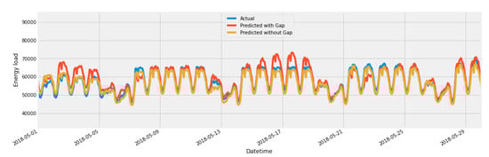
Figure 21.
Comparison of hybrid model with and without imputation.
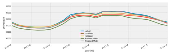
Figure 22.
Comparison of purposed model with ensemble models.
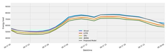
Figure 23.
Comparison of purposed model with ARIMA, GRU, and LSTM.
8. Conclusions
The main contributions of this article are presenting a Hybrid ML algorithm for energy prediction and data imputation technique for the large gap in the dataset. The approach for data imputation heavily depends upon the nature of data. We can not select the imputation method randomly. We analyze and perform EDA on our dataset before applying the proposed hybrid model. We found that in comparison to the model with missing data, our proposed hybrid model with imputed data is much better. The prediction results of the proposed model are better than individual algorithms. We also performed pre-processing of data and feature selection and made the correlation graph. After applying the proposed algorithms, we make graphs to visualize the results and report the test score of the best model. We compared our proposed model against the existing benchmark models. The proposed model can be used for forecasting for any other dataset as well. In future recurrent neural network algorithms can also be added to make the performance more robust. We have used time-series features but in further studies, other features including temperature, humidity, wind speed, holidays can also be added and a genetic algorithm can also be used for feature selection.
Author Contributions
Conceptualization, P.W.K.; Formal analysis, P.W.K.; Funding acquisition, Y.-C.B.; Methodology, S.-J.L.; Writing–review and editing, S.-J.L.; Investigation, N.P.; Resources, N.P.; Methodology, P.W.K.; Project administration, Y.-C.B.; Supervision, Y.-C.B. All authors have read and agreed to the published version of the manuscript.
Funding
This work was supported by Institute for Information & communications Technology Promotion(IITP) grant funded by the Korea government(MSIT) [2019-0-00203, The Development of Predictive Visual Security Technology for Preemptive Threat Response]. And, This work was supported by the Ministry of Education of the Republic of Korea and the National Research Foundation of Korea (NRF-2019S1A5C2A04083374).
Conflicts of Interest
The authors declare no conflict of interest regarding the design of this study, analyses and writing of this manuscript.
Abbreviations
The following abbreviations are used in this manuscript:
| ML | Machine Learning |
| RPS | Renewable Energy Portfolio Standard |
| FIT | Feed-in-Tariff |
| ANN | Artificial Neural Network |
| RMSE | Root Mean Square Error |
| NARX | Nonlinear Auto-regressive Exogenous |
| MLP | Multi-Layer Perceptron |
| DOPH | Direct Optimum Parallel Hybrid |
| SARIMA | Seasonal Autoregressive Integrated Moving Average |
| ARMA | Auto-Regressive Moving Average |
| ANFIS | Adaptive Network-based Fuzzy Inference System |
| DE | Differential Evolution |
| GA | Genetic Algorithm |
| NSGA | Nondominated Sorting Genetic Algorithm |
| EMD | Empirical Mode Decomposition |
| ELM | Extreme Learning Machine |
| IMFs | Intrinsic Mode Entropy |
| DBN | Deep Belief Network |
| MCAR | Missing Completely at Random |
| MAR | Missing at Random |
| NMAR | Not Missing at Random |
| MAE | Mean Absolute Error |
| EEMD | Ensemble Empirical Mode Decomposition |
References
- Aler, R.; Huertas-Tato, J.; Valls, J.M.; Galván, I.M. Improving Prediction Intervals Using Measured Solar Power with a Multi-Objective Approach. Energies 2019, 12, 4713. [Google Scholar] [CrossRef]
- Connolly, R.; Connolly, M.; Carter, R.M.; Soon, W. How Much Human-Caused Global Warming Should We Expect with Business-As-Usual (BAU) Climate Policies? A Semi-Empirical Assessment. Energies 2020, 13, 1365. [Google Scholar] [CrossRef]
- Zhang, P.; Ma, X.; She, K. Forecasting Japan’s Solar Energy Consumption Using a Novel Incomplete Gamma Grey Model. Sustainability 2019, 11, 5921. [Google Scholar] [CrossRef]
- Kim, T.; Ko, W.; Kim, J. Analysis and Impact Evaluation of Missing Data Imputation in Day-ahead PV Generation Forecasting. Appl. Sci. 2019, 9, 204. [Google Scholar]
- Chen, T.; Guestrin, C. Xgboost: A scalable tree boosting system. In Proceedings of the 22nd ACM Sigkdd International Conference on Knowledge Discovery and Data Mining, New York, NY, USA, 13–17 August 2016; pp. 785–794. [Google Scholar]
- Breiman, L. Random forests. Mach. Learn. 2001, 45, 5–32. [Google Scholar]
- Dorogush, A.V.; Ershov, V.; Gulin, A. CatBoost: Gradient boosting with categorical features support. arXiv 2018, arXiv:1810.11363. [Google Scholar]
- Daut, M.A.M.; Hassan, M.Y.; Abdullah, H.; Rahman, H.A.; Abdullah, M.P.; Hussin, F. Building electrical energy consumption forecasting analysis using conventional and artificial intelligence methods: A review. Renew. Sustain. Energy Rev. 2017, 70, 1108–1118. [Google Scholar] [CrossRef]
- Jeju Special Self-Governing Province. Carbon Free Island Jeju by 2030. Available online: http://www.investkorea.org/jeju_en/about/cfi2030.do (accessed on 3 April 2020).
- Huh, S.Y.; Lee, J.; Shin, J. The economic value of South Korea renewable energy policies (RPS, RFS, and RHO): A contingent valuation study. Renew. Sustain. Energy Rev. 2015, 50, 64–72. [Google Scholar] [CrossRef]
- Lee, S.; Cha, J.; Kim, M.K.; Kim, K.S.; Pham, V.H.; Leach, M. Neural-Network-Based Building Energy Consumption Prediction with Training Data Generation. Processes 2019, 7, 731. [Google Scholar] [CrossRef]
- Kim, M.; Jung, S.; Kang, J.w. Artificial Neural Network-Based Residential Energy Consumption Prediction Models Considering Residential Building Information and User Features in South Korea. Sustainability 2020, 12, 109. [Google Scholar] [CrossRef]
- Niu, M.; Sun, S.; Wu, J.; Yu, L.; Wang, J. An innovative integrated model using the singular spectrum analysis and nonlinear multi-layer perceptron network optimized by hybrid intelligent algorithm for short-term load forecasting. Appl. Math. Model. 2016, 40, 4079–4093. [Google Scholar] [CrossRef]
- Yang, Y.; Chen, Y.; Wang, Y.; Li, C.; Li, L. Modelling a combined method based on ANFIS and neural network improved by DE algorithm: A case study for short-term electricity demand forecasting. Appl. Soft Comput. 2016, 49, 663–675. [Google Scholar] [CrossRef]
- Raza, M.; Nadarajah, M.; Quoc Hung, D.; Baharudin, Z. An intelligent hybrid short term load forecast model for seasonal prediction of smart power grid. Sustain. Cities Soc. 2016, 10, 264–275. [Google Scholar]
- Monjoly, S.; André, M.; Calif, R.; Soubdhan, T. Hourly forecasting of global solar radiation based on multiscale decomposition methods: A hybrid approach. Energy 2017, 119, 288–298. [Google Scholar] [CrossRef]
- Zhang, X.; Wang, J.; Zhang, K. Short-term electric load forecasting based on singular spectrum analysis and support vector machine optimized by Cuckoo search algorithm. Electr. Power Syst. Res. 2017, 146, 270–285. [Google Scholar] [CrossRef]
- Sharifian, A.; Ghadi, M.J.; Ghavidel, S.; Li, L.; Zhang, J. A new method based on Type-2 fuzzy neural network for accurate wind power forecasting under uncertain data. Renew. Energy 2018, 120, 220–230. [Google Scholar] [CrossRef]
- Dehghani, M.; Riahi-Madvar, H.; Hooshyaripor, F.; Mosavi, A.; Shamshirband, S.; Zavadskas, E.K.; Chau, K.W. Prediction of hydropower generation using grey wolf optimization adaptive neuro-fuzzy inference system. Energies 2019, 12, 289. [Google Scholar] [CrossRef]
- Bissing, D.; Klein, M.T.; Chinnathambi, R.A.; Selvaraj, D.F.; Ranganathan, P. A hybrid regression model for day-ahead energy price forecasting. IEEE Access 2019, 7, 36833–36842. [Google Scholar] [CrossRef]
- Ma, M.; Wang, Z. Prediction of the Energy Consumption Variation Trend in South Africa based on ARIMA, NGM and NGM-ARIMA Models. Energies 2020, 13, 10. [Google Scholar] [CrossRef]
- Ahmad, A.; Anderson, T.; Lie, T. Hourly global solar irradiation forecasting for New Zealand. Sol. Energy 2015, 122, 1398–1408. [Google Scholar] [CrossRef]
- Chahkoutahi, F.; Khashei, M. A seasonal direct optimal hybrid model of computational intelligence and soft computing techniques for electricity load forecasting. Energy 2017, 140, 988–1004. [Google Scholar] [CrossRef]
- Zhao, Z.; Xu, Y.; Zhao, Y. SXGBsite: Prediction of Protein–Ligand Binding Sites Using Sequence Information and Extreme Gradient Boosting. Genes 2019, 10, 965. [Google Scholar] [CrossRef] [PubMed]
- Jin, Q.; Fan, X.; Liu, J.; Xue, Z.; Jian, H. Using eXtreme Gradient BOOSTing to Predict Changes in Tropical Cyclone Intensity over the Western North Pacific. Atmosphere 2019, 10, 341. [Google Scholar] [CrossRef]
- Deng, S.; Wang, C.; Li, J.; Yu, H.; Tian, H.; Zhang, Y.; Cui, Y.; Ma, F.; Yang, T. Identification of Insider Trading Using Extreme Gradient Boosting and Multi-Objective Optimization. Information 2019, 10, 367. [Google Scholar] [CrossRef]
- Lahouar, A.; Slama, J.B.H. Day-ahead load forecast using random forest and expert input selection. Energy Convers. Manag. 2015, 103, 1040–1051. [Google Scholar] [CrossRef]
- Zhang, F.; Fleyeh, H. Short Term Electricity Spot Price Forecasting Using CatBoost and Bidirectional Long Short Term Memory Neural Network. In Proceedings of the 2019 16th International Conference on the European Energy Market (EEM), Ljubljana, Slovenia, 18–20 September 2019; pp. 1–6. [Google Scholar]
- Deng, B.; Peng, D.; Zhang, H.; Qian, Y. An intelligent hybrid short-term load forecasting model optimized by switching delayed PSO of micro-grids. J. Renew. Sustain. Energy 2018, 10, 024901. [Google Scholar] [CrossRef]
- Fu, G. Deep belief network based ensemble approach for cooling load forecasting of air-conditioning system. Energy 2018, 148, 269–282. [Google Scholar] [CrossRef]
- Yoo, K.; Park, E.; Kim, H.; Ohm, J.; Yang, T.; Kim, K.; Chang, H.; del Pobil, A. Optimized renewable and sustainable electricity generation systems for Ulleungdo Island in South Korea. Sustainability 2014, 6, 7883–7893. [Google Scholar] [CrossRef]
- Bae, K.; Shim, J.H. Economic and environmental analysis of a wind-hybrid power system with desalination in Hong-do, South Korea. Int. J. Precis. Eng. Manuf. 2012, 13, 623–630. [Google Scholar] [CrossRef]
- Park, E.; Kim, K.; Kwon, S.; Han, T.; Na, W.; del Pobil, A. Economic feasibility of renewable electricity generation systems for local government office: Evaluation of the Jeju special self-governing Province in South Korea. Sustainability 2017, 9, 82. [Google Scholar] [CrossRef]
- Chen, T.; He, T.; Benesty, M.; Khotilovich, V.; Tang, Y. Xgboost: Extreme Gradient Boosting; R Package Version 0.4-2; 2015. Available online: http://cran.fhcrc.org/web/packages/xgboost/vignettes/xgboost.pdf (accessed on 13 December 2019).
- Chen, J.; Yin, J.; Zang, L.; Zhang, T.; Zhao, M. Stacking machine learning model for estimating hourly PM2.5 in China based on Himawari 8 aerosol optical depth data. Sci. Total Environ. 2019, 697, 134021. [Google Scholar] [CrossRef] [PubMed]
- Ghori, K.M.; Abbasi, R.A.; Awais, M.; Imran, M.; Ullah, A.; Szathmary, L. Performance Analysis of Different Types of Machine Learning Classifiers for Non-Technical Loss Detection. IEEE Access 2019, 8, 16033–16048. [Google Scholar] [CrossRef]
- De Clercq, D.; Wen, Z.; Fei, F.; Caicedo, L.; Yuan, K.; Shang, R. Interpretable machine learning for predicting biomethane production in industrial-scale anaerobic co-digestion. Sci. Total Environ. 2020, 712. [Google Scholar] [CrossRef]
- Liu, J.; Wang, X.; Lu, Y. A novel hybrid methodology for short-term wind power forecasting based on adaptive neuro-fuzzy inference system. Renew. Energy 2017, 103, 620–629. [Google Scholar] [CrossRef]
- De, G.; Gao, W. Forecasting China’s Natural Gas Consumption Based on AdaBoost-Particle Swarm Optimization-Extreme Learning Machine Integrated Learning Method. Energies 2018, 11, 2938. [Google Scholar]
- Lin, J.; Shi, W. Statistical Correlation between Monthly Electric Power Consumption and VIIRS Nighttime Light. ISPRS Int. J. Geo-Inf. 2020, 9, 32. [Google Scholar] [CrossRef]
© 2020 by the authors. Licensee MDPI, Basel, Switzerland. This article is an open access article distributed under the terms and conditions of the Creative Commons Attribution (CC BY) license (http://creativecommons.org/licenses/by/4.0/).