Aerodynamic Performance Analysis of a Building-Integrated Savonius Turbine

Abstract
1. Introduction
- The average power of the turbine decreases with increasing turbine gap.
- The average Cp of the turbine under 360-degree wind angles is 0.4256.
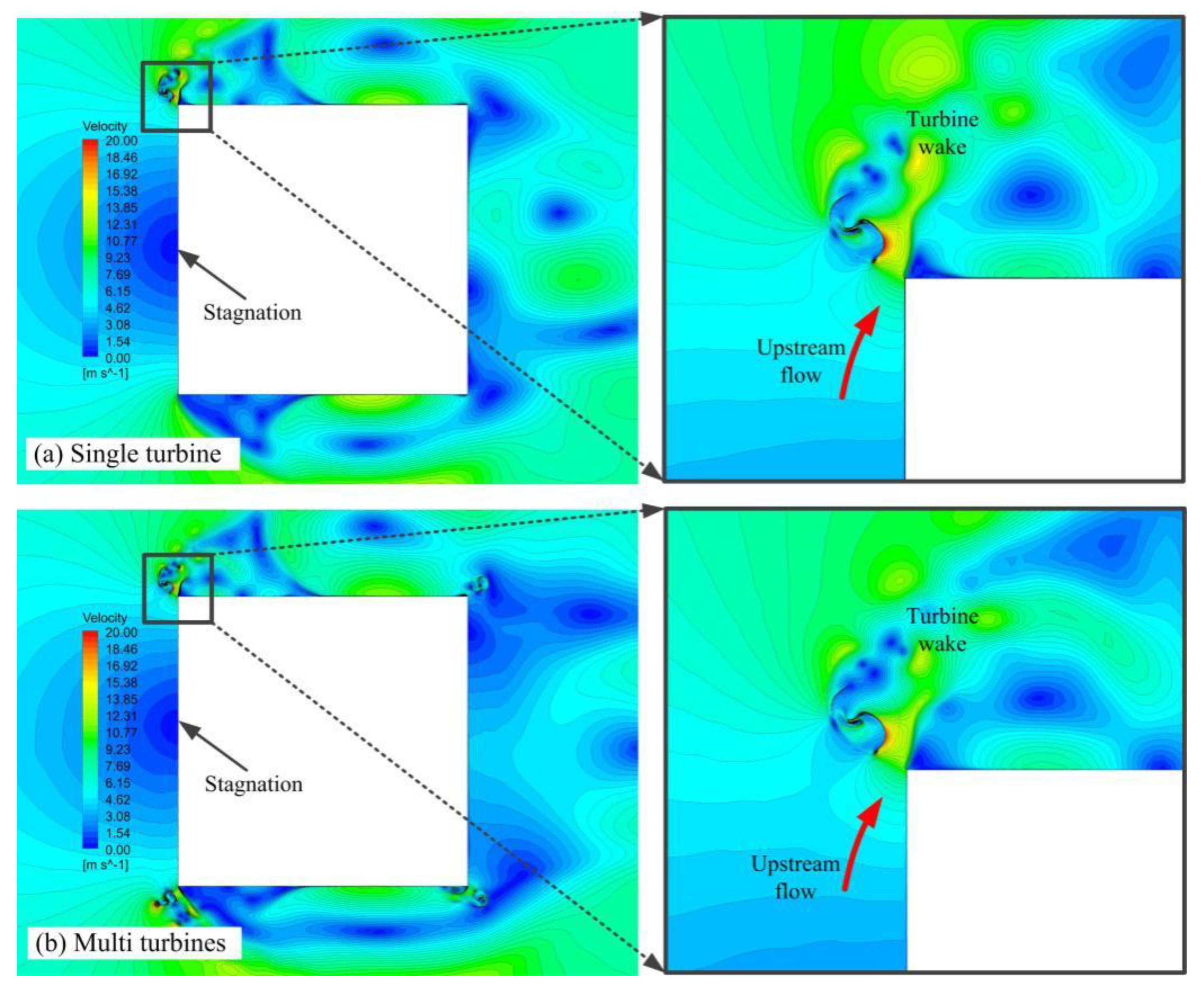
- Adjacent turbines directly leads to a decrease in the velocity of flow upstream of the turbine.
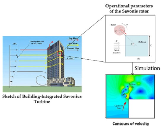
2. Problem Description
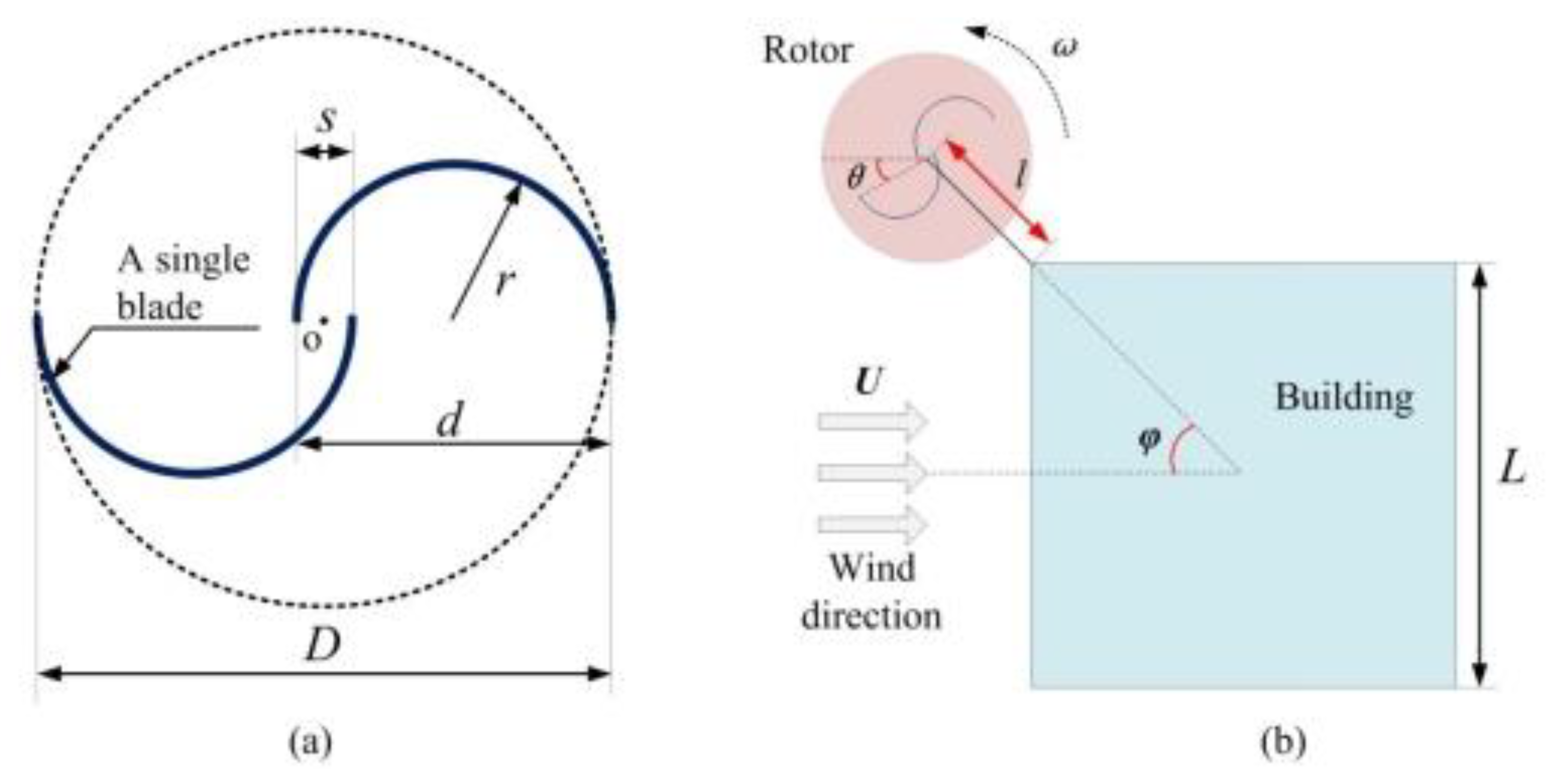
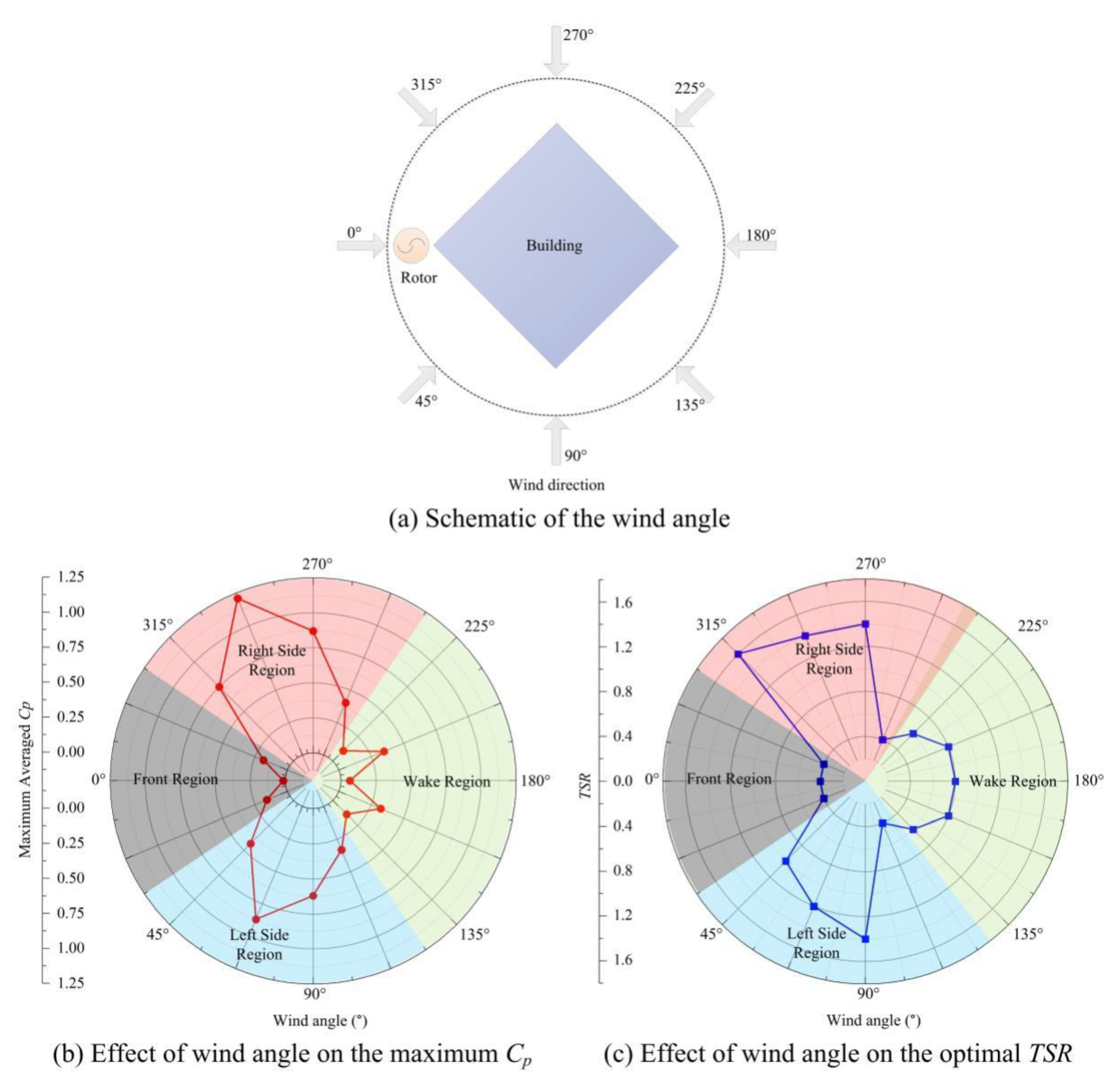
2.1. Parameter Definition
- (1)
- The building is tall enough so that the vertical velocity components of the side flow is zero.
- (2)
- The height of the wind turbine is negligibly small compared with that of the building, hence the velocity of the flow upstream of the turbine can be treated as uniform.
2.2. Coefficients for Performance
2.3. Simulation Cases
3. Numerical Method
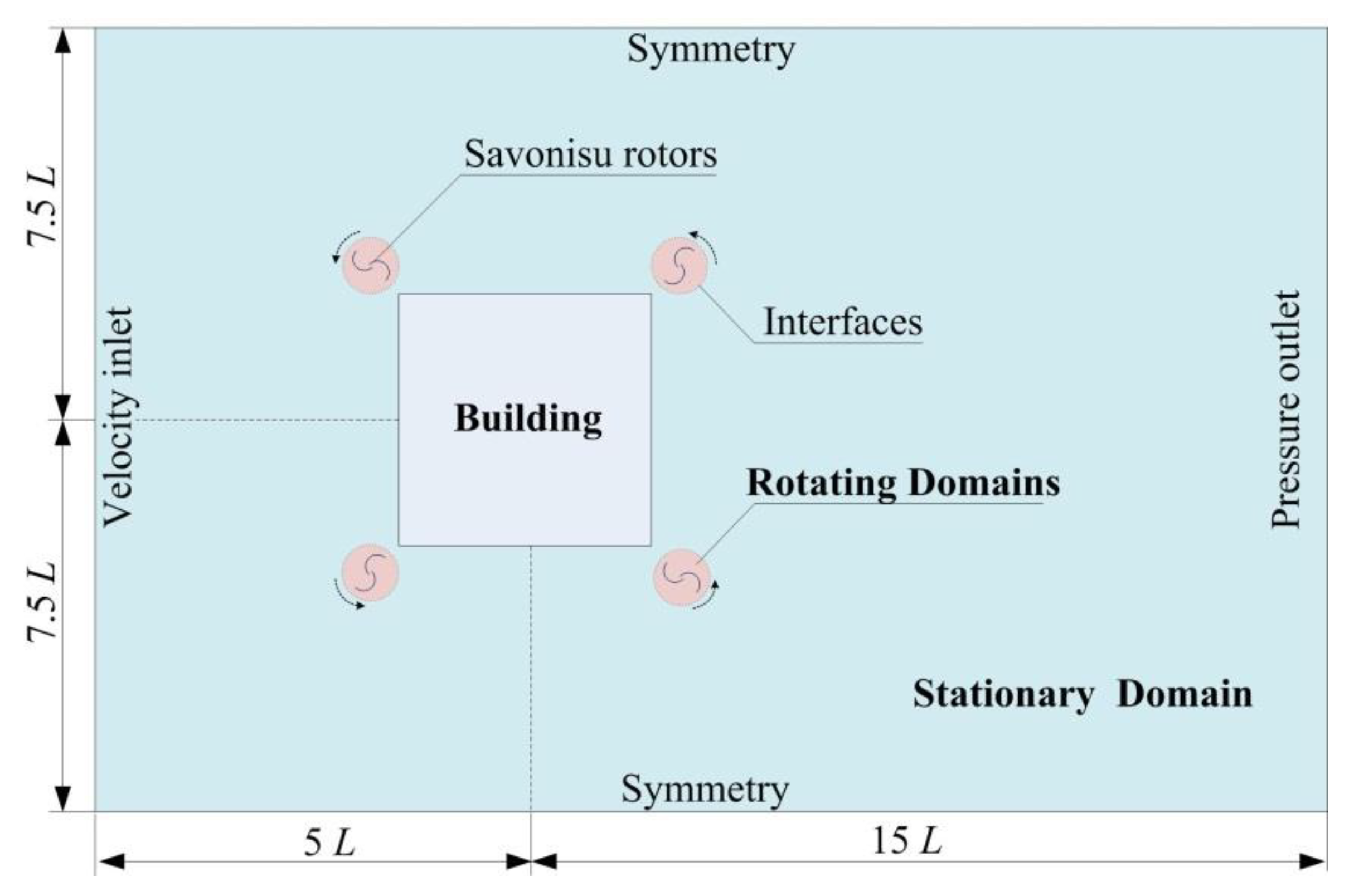
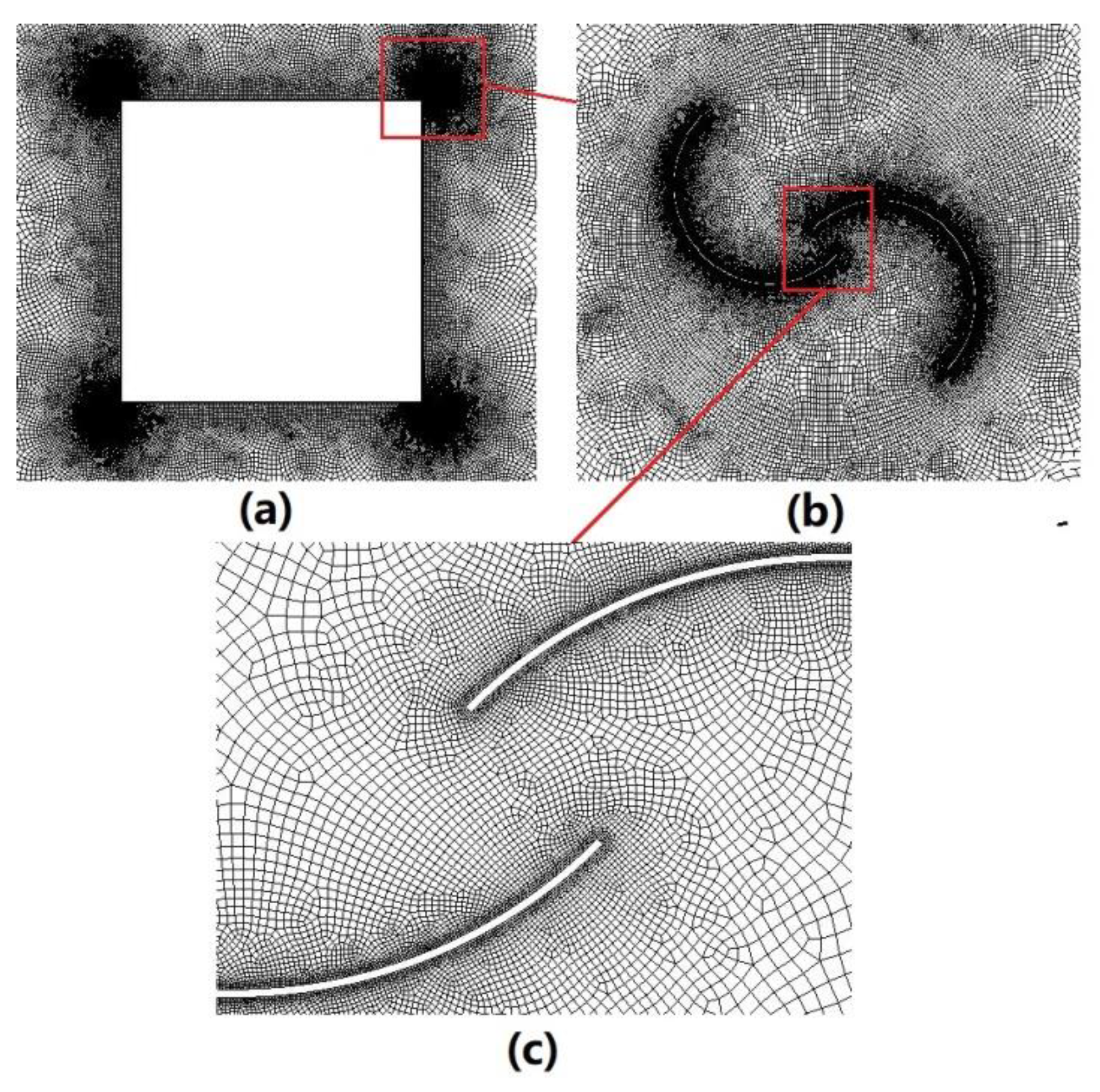
3.1. Computational Domains and Grid Generation
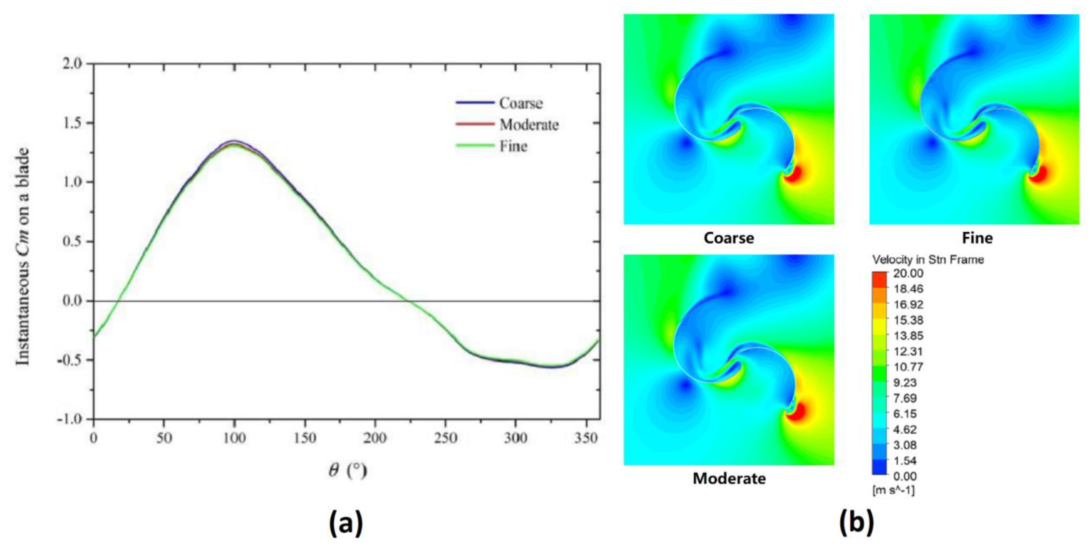
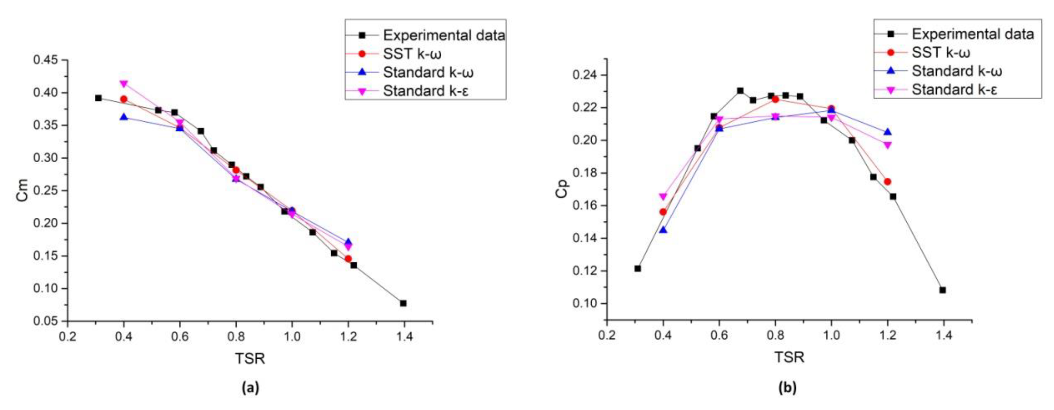
3.2. Numerical Method Validation
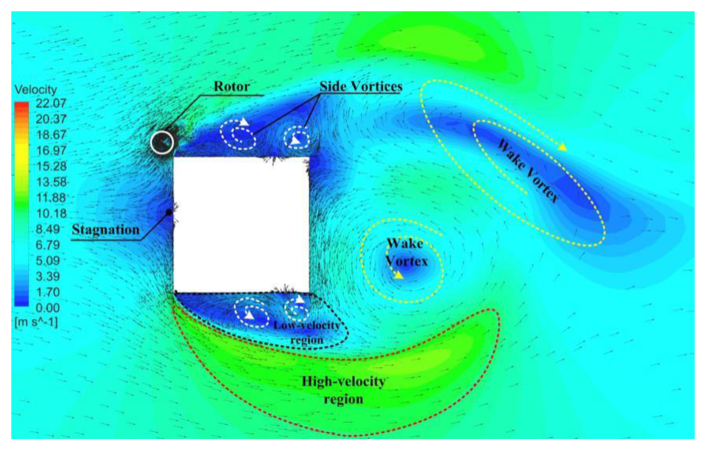
- (1)
- Stagnation: the stagnation point on the surface of the building with zero velocity.
- (2)
- High-Velocity Region: regions around the two sides of the building where the flow is deflected and accelerated.
- (3)
- Low-Velocity Region: regions between the High-Velocity Region and the sides of the building where small side vortices exist and the velocity is decreased.
- (4)
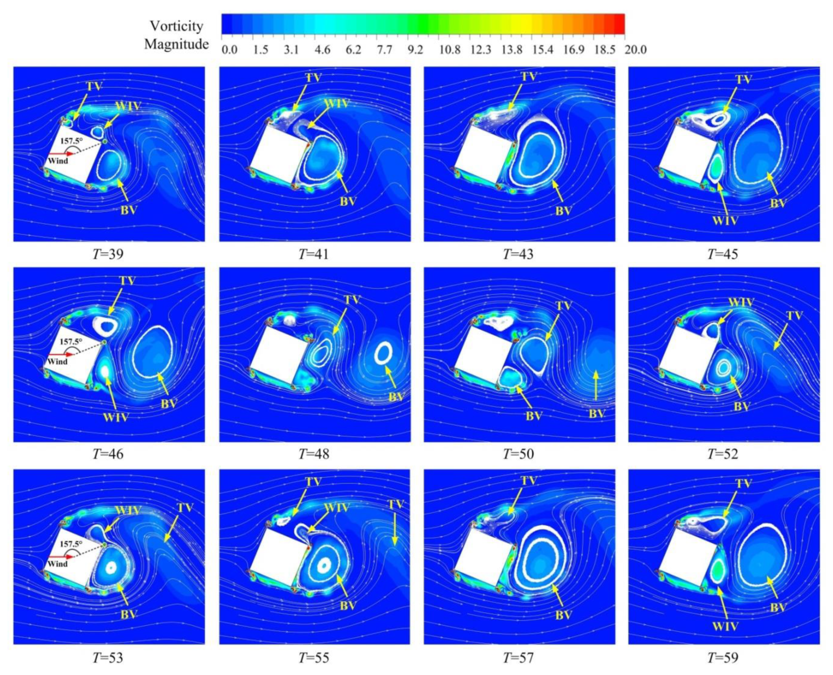
- Wake Vortices: vortices periodically shed from the corners of the building which have significant effects on the flow near the rear surface of the building.
4. Results and Discussion
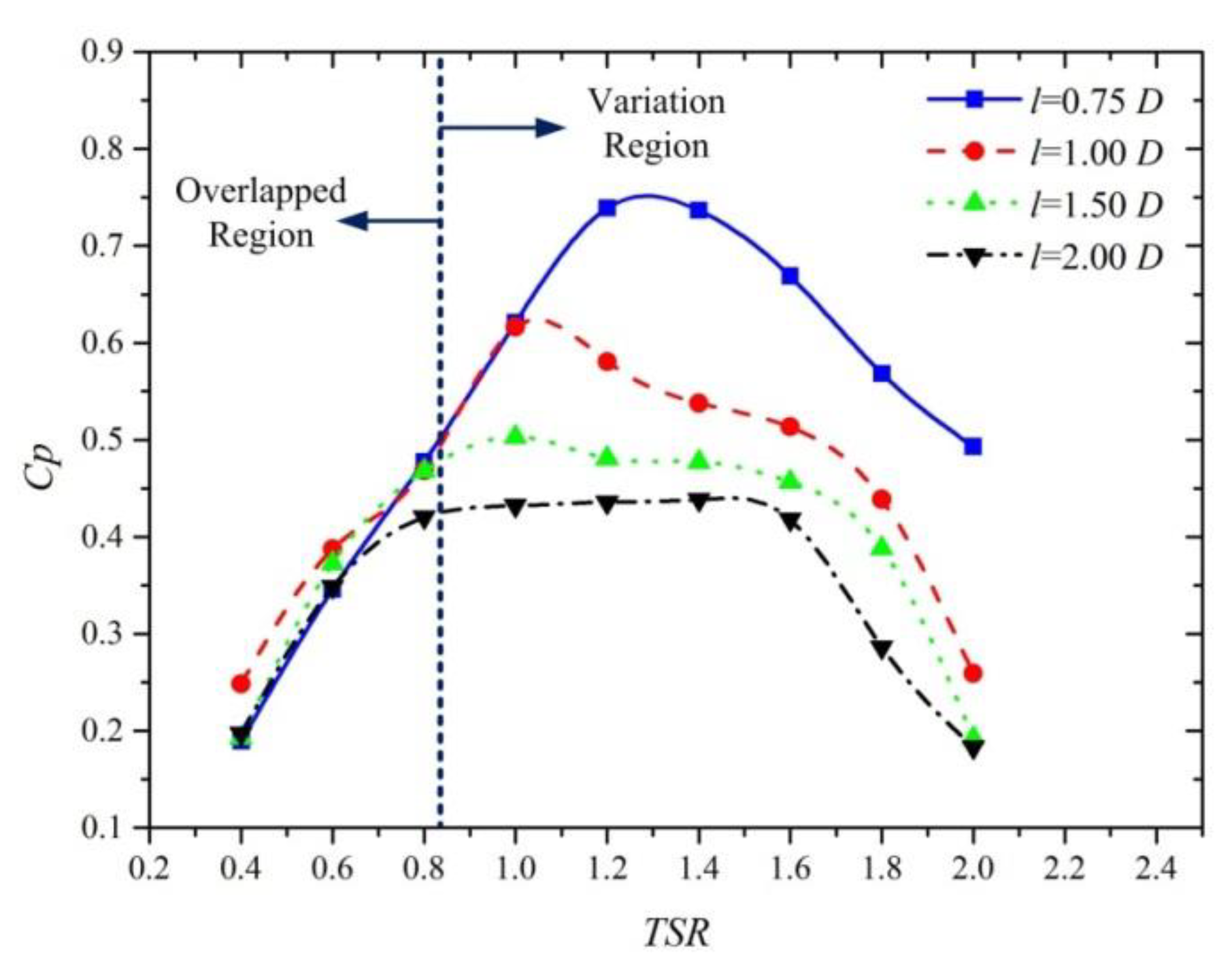
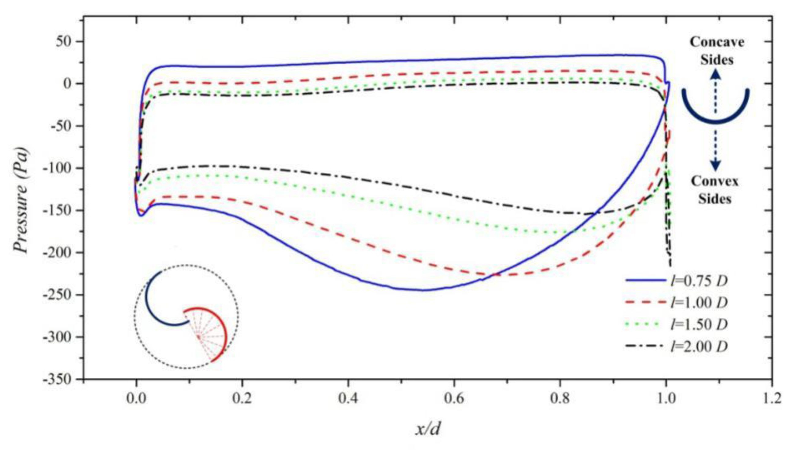
4.1. Effects of Gap on the Performance of the Turbine
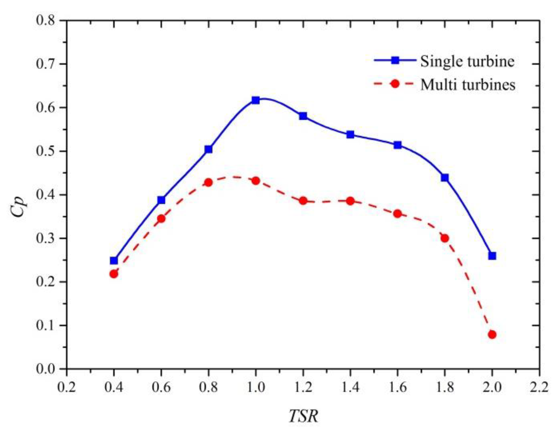
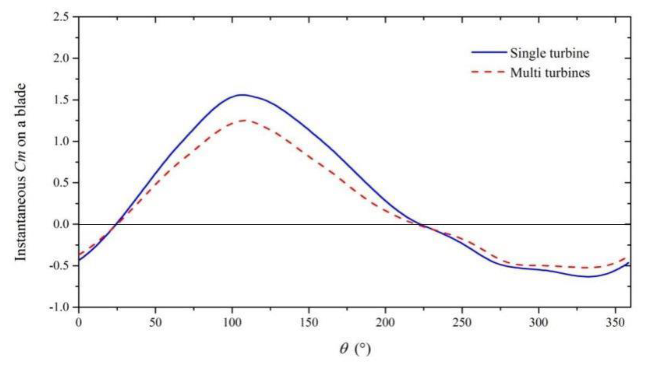
4.2. Effect of Adjacent Turbines on the Performance of the Turbine
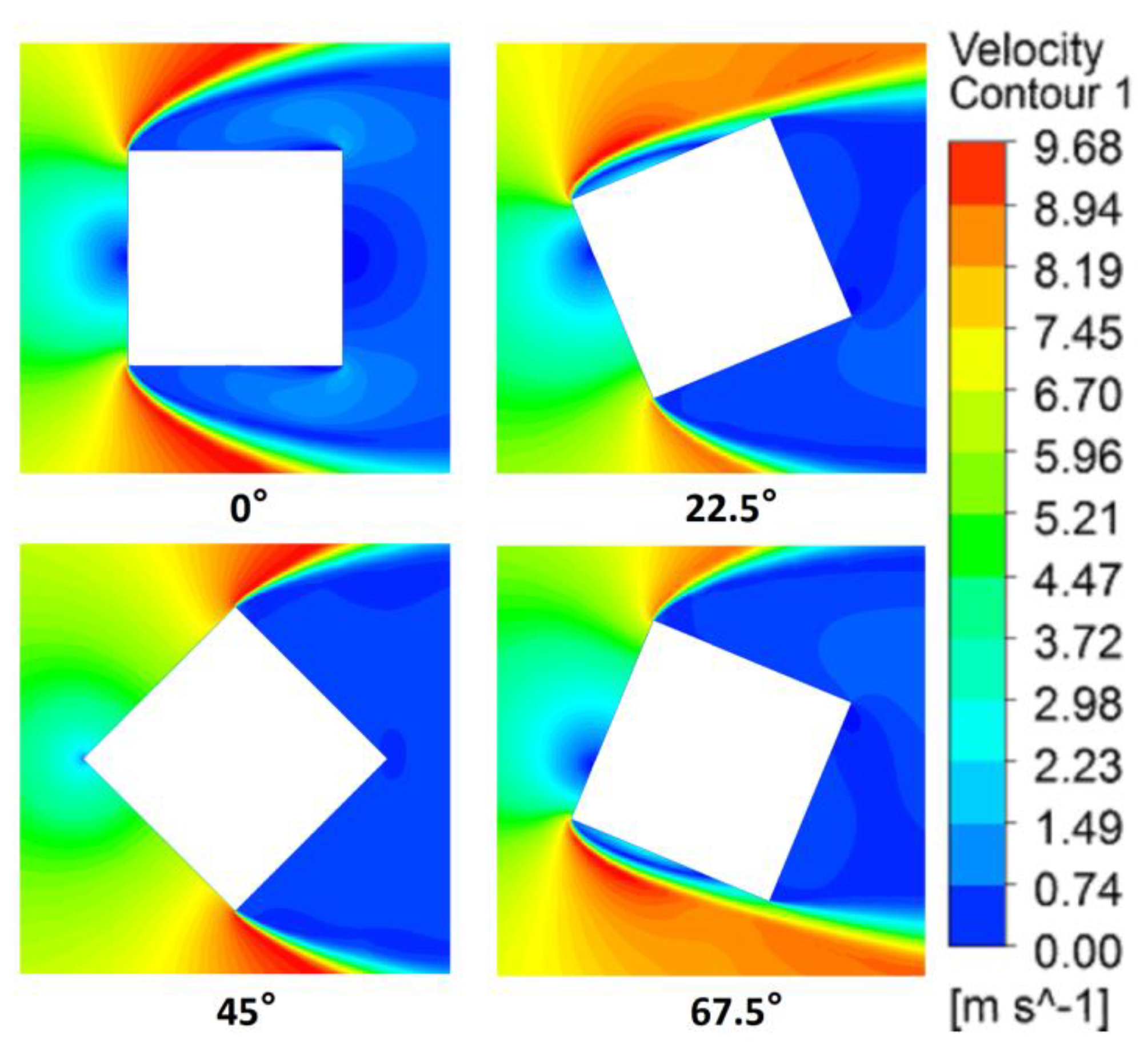
4.3. Effect of Wind Angle on the Performance of the Turbine
4.3.1. Front Region
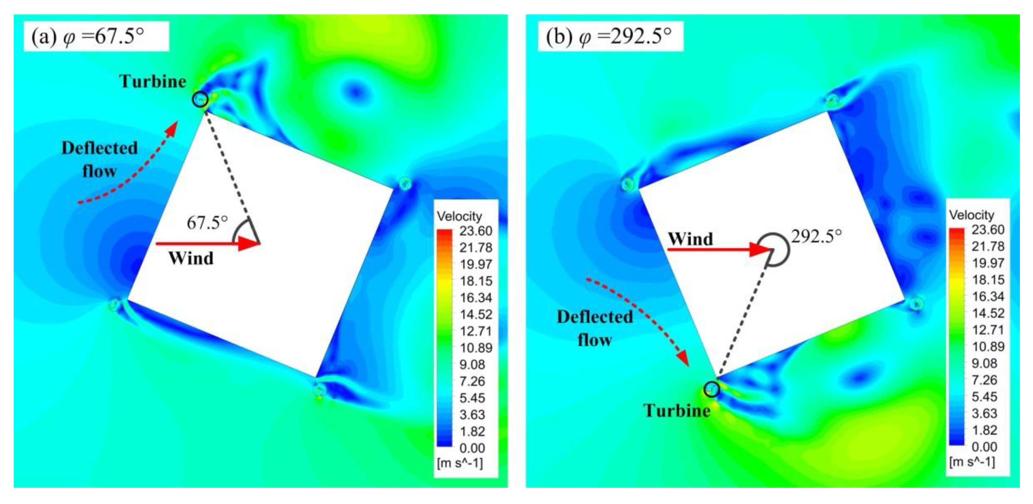
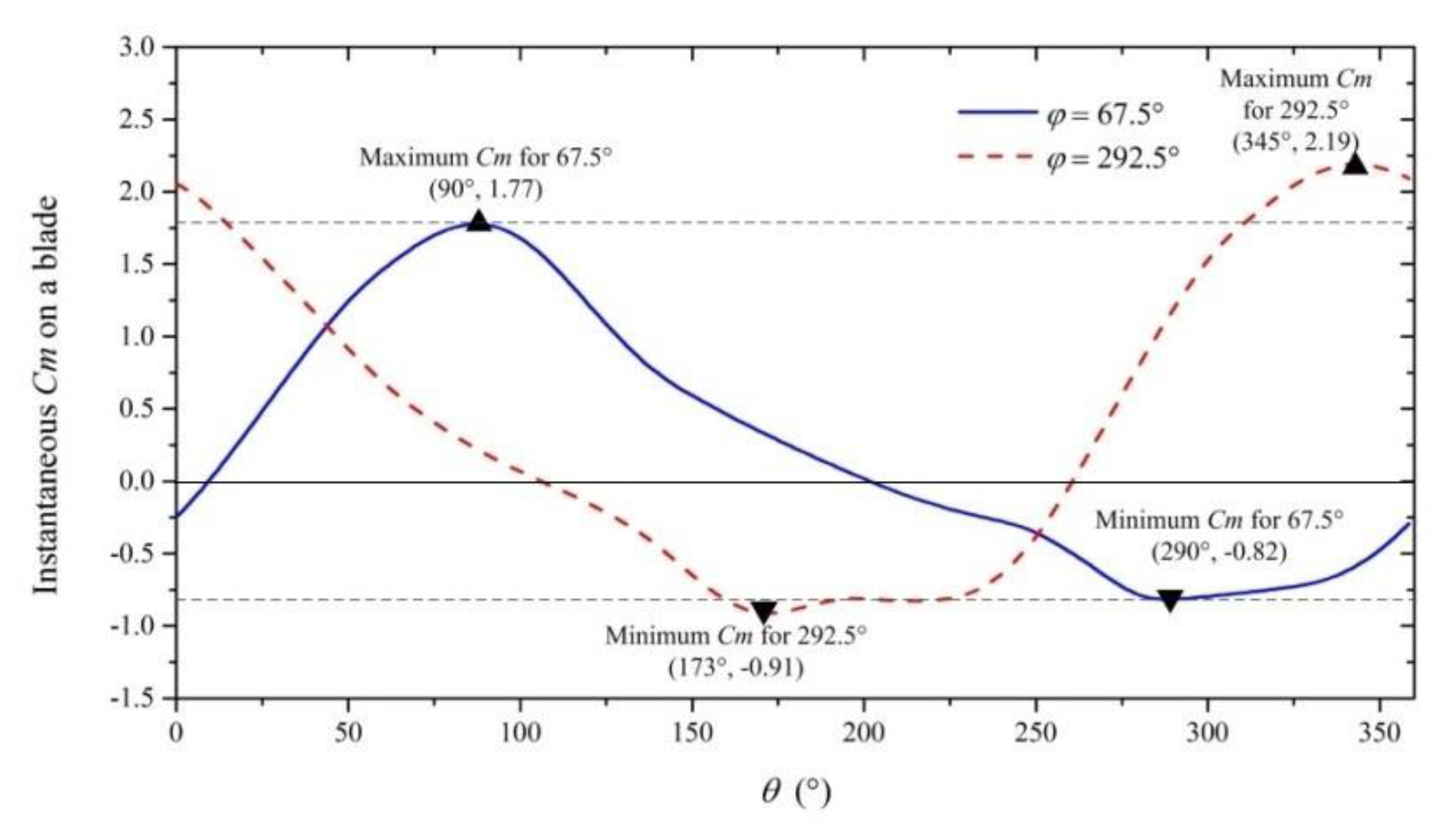
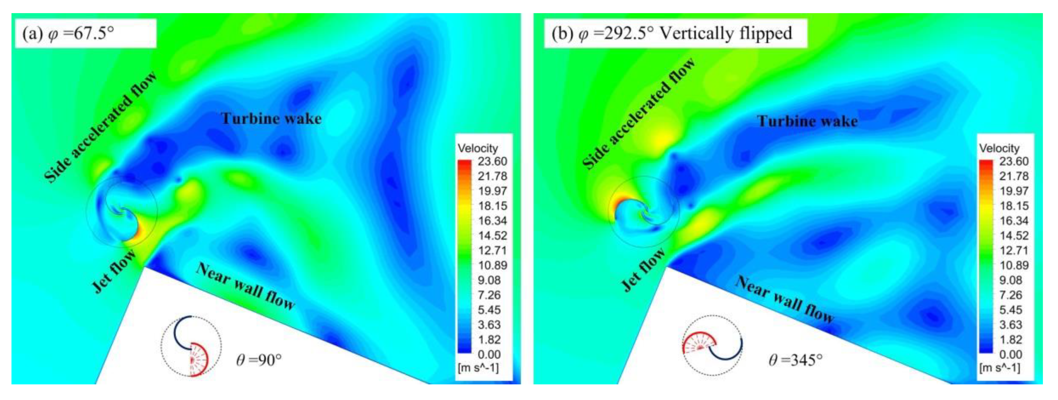
4.3.2. Left Side Region and Right Side Region
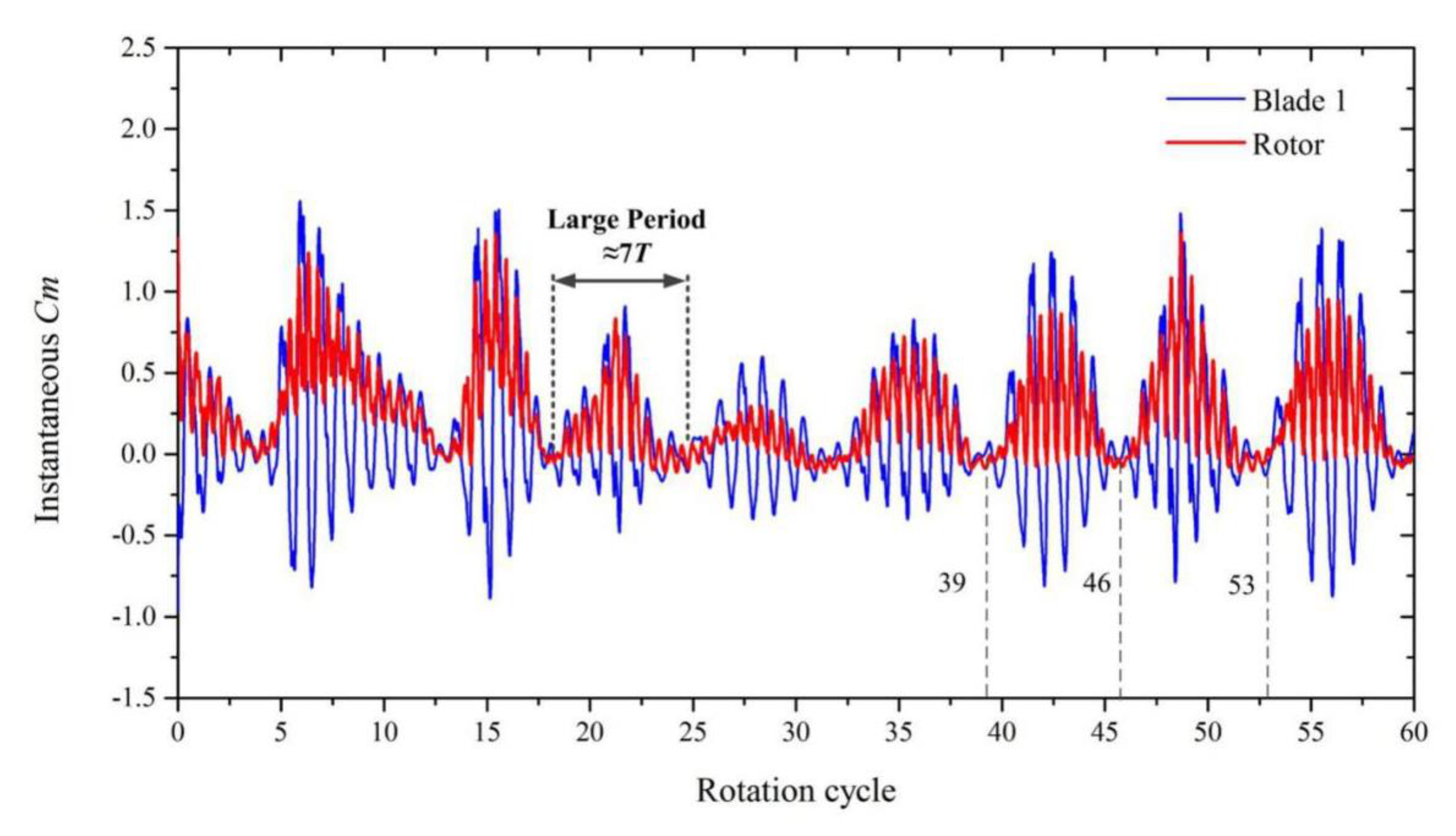
4.3.3. Wake Region
5. Conclusions
- (1)
- The average power of the turbine decreases with the increasing turbine gap, mainly because the gap changes the Jet Flow and Recovery flow. The maximum Cp of the building-integrated turbine, 0.7390 at l = 0.75 D and TSR = 1.2, is 234.4% higher than the Savonius turbine operating in uniform flows.
- (2)
- The maximum Cp for multi-turbines is 0.4319, and is 29.2% lower than that of a single turbine at l = 1.00 D and φ = 45°. Even so, it is still much higher than that of the turbine rotating in uniform wind flows.
- (3)
- Wind angle has a significant influence on the power output of the turbine. The average Cp of the turbine under 360-degree wind angles is 0.4256, which is 92.5% higher than the turbine operating in uniform flows. This means that Savonius turbine has better performance if installed on a building.
- (4)
- The turbine in the Front Region has the lowest coefficients of power. That is because the turbine locates just in the stagnation region, where the flow velocity is very low.
- (5)
- The turbine has higher coefficients of power in the Left Side Region and the Right Side Region, with a maximum Cp of 1.2093 obtained in the Right Side Region.
- (6)
- The turbine in the Wake Region is affected by the periodic vortices shed from the building corners and the transient torque shows a periodic fluctuation.
- (7)
- The influences of wind angle on the performance of the turbine are the most significant. When the turbine gap is smaller, it also improves the performance of the turbine. Compared to a single turbine, the effect of adjacent turbines on turbine performance is negative.
Author Contributions
Funding
Conflicts of Interest
References
- Stankovic, S.; Campbell, N.; Harries, A. Urban Wind Energy; Earthscan: London, UK, 2009. [Google Scholar]
- Peacock, A.D.; Jenkins, D.; Ahadzi, M.; Berry, A.; Turan, S. Micro wind turbines in the UK domestic sector. Energy Build. 2008, 40, 1324–1333. [Google Scholar] [CrossRef]
- Ledo, L.; Kosasih, P.B.; Cooper, P. Roof mounting site analysis for micro-wind turbines. Renew. Energy 2011, 36, 1379–1391. [Google Scholar] [CrossRef]
- Blackmore, P. Building-mounted Micro-wind Turbines on High-rise and Commercial Buildings: (FB 22). Appl. Biochem. Biotechnol. 2010, 89, 1–13. [Google Scholar]
- Toja-Silva, F.; Colmenar-Santos, A.; Castro-Gil, M. Urban wind energy exploitation systems: Behaviour under multidirectional flow conditions—Opportunities and challenges. Renew. Sustain. Energy Rev. 2013, 24, 364–378. [Google Scholar] [CrossRef]
- Rafailidis, S. Influence of Building Areal Density and Roof Shape on the Wind Characteristics Above a Town. Bound. Layer Meteorol. 1997, 85, 255–271. [Google Scholar] [CrossRef]
- Abohela, I.; Hamza, N.; Dudek, S. Effect of roof shape, wind direction, building height and urban configuration on the energy yield and positioning of roof mounted wind turbines. Renew. Energy 2013, 50, 1106–1118. [Google Scholar] [CrossRef]
- Bobrova, D. Building-Integrated Wind Turbines in the Aspect of Architectural Shaping. Procedia Eng. 2015, 117, 404–410. [Google Scholar] [CrossRef]
- Larin, P.; Paraschivoiu, M.; Aygun, C. CFD based synergistic analysis of wind turbines for roof mounted integration. J. Wind Eng. Ind. Aerodyn. 2016, 156, 1–13. [Google Scholar] [CrossRef]
- Tian, W.; Mao, Z.; Zhang, B.; Li, Y. Shape Optimization of a Savonius Wind Rotor with Different Convex and Concave Sides. Renew. Energy 2018, 117, 287–299. [Google Scholar] [CrossRef]
- Pope, K.; Dincer, I.; Naterer, G.F. Energy and exergy efficiency comparison of horizontal and vertical axis wind turbines. Renew. Energy 2010, 35, 2102–2113. [Google Scholar] [CrossRef]
- Shigetomi, A.; Murai, Y.; Tasaka, Y.; Takeda, Y. Interactive flow field around two Savonius turbines. Renew. Energy 2011, 36, 536–545. [Google Scholar] [CrossRef]
- Sivasegaram, S. Design parameters affecting the performance of resistance-type, vertical-axis windrotors—An experimental investigation. Wind Eng. 1977, 1, 8. [Google Scholar]
- Akwa, J.V.; Vielmo, H.A.; Petry, A.P. A review on the performance of Savonius wind turbines. Renew. Sustain. Energy Rev. 2012, 16, 3054–3064. [Google Scholar] [CrossRef]
- Altan, B.D.; Atılgana, M.; Özdamarb, A. An experimental study on improvement of a Savonius rotor performance with curtaining. Exp. Therm. Fluid Sci. 2008, 32, 1673–1678. [Google Scholar] [CrossRef]
- Zhao, Z.; Zheng, Y.; Xu, X.; Liu, W. Research on the improvement of the performance of savonius rotor based on numerical study. In Proceedings of the International Conference on Sustainable Power Generation and Supply, Nanjing, China, 6–7 April 2009; pp. 1–6. [Google Scholar]
- Kerikous, E.; Thevenin, D. Optimal shape of thick blades for a hydraulic Savonius turbine. Renew. Energy 2019, 134, 629–638. [Google Scholar] [CrossRef]
- Chan, C.M.; Bai, H.L.; He, D.Q. Blade shape optimization of the Savonius wind turbine using a genetic algorithm. Appl. Energy 2018, 213, 148–157. [Google Scholar] [CrossRef]
- Kumar, A.; Saini, R.P. Performance analysis of a single stage modified Savonius hydrokinetic turbine having twisted blades. Renewable Energy. 2017, 113, 461–478. [Google Scholar] [CrossRef]
- Sharma, S.; Sharma, R.K. Performance improvement of Savonius rotor using multiple quarter blades—A CFD investigation. Energy Convers. Manag. 2016, 127, 43–54. [Google Scholar] [CrossRef]
- Yang, Y.; Gu, M.; Chen, S.; Jin, X. New inflow boundary conditions for modelling the neutral equilibrium atmospheric boundary layer in computational wind engineering. J. Wind Eng. Ind. Aerodyn. 2009, 97, 88–95. [Google Scholar] [CrossRef]
- Shamsoddin, S.; Portéagel, F. A Large-eddy Simulation Study of Vertical Axis Wind Turbine Wakes in the Atmospheric Boundary Layer. Energies 2016, 9, 366. [Google Scholar] [CrossRef]
- Sheldahl, R.E.; Feltz, L.V.; Blackwell, B.F. Wind tunnel performance data for two- and three-bucket Savonius rotors. J. Energy 1978, 2, 160–164. [Google Scholar] [CrossRef]
- Kacprzak, K.; Liskiewicz, G.; Sobczak, K. Numerical investigation of conventional and modified Savonius wind turbines. Renew. Energy 2013, 60, 578–585. [Google Scholar] [CrossRef]
- Mohamed, M.H.; Janiga, G.; Pap, E.; Thévenin, D. Optimal blade shape of a modified Savonius turbine using an obstacle shielding the returning blade. Energy Convers. Manag. 2011, 52, 236–242. [Google Scholar] [CrossRef]


| Parameter | Value | Parameter | Value |
|---|---|---|---|
| D | 0.91 m | U | 7 m/s |
| d | 0.50 m | l | variable |
| r | 0.25 m | φ | variable |
| S | 0.09 m | ω | variable |
| L | 15.00 m | θ | variable |
| Group | Key Factors | l | φ | Number of Turbines | TSR |
|---|---|---|---|---|---|
| 1 | Turbine gap | 0.75 D–2.00 D | 45° | 1 | 0.4–2.0 |
| 2 | Adjacent turbines | 1.00 D | 45° | 4 | 0.4–2.0 |
| 3 | Wind direction | 1.00 D | 0°–360° | 4 | 0.4–2.0 |
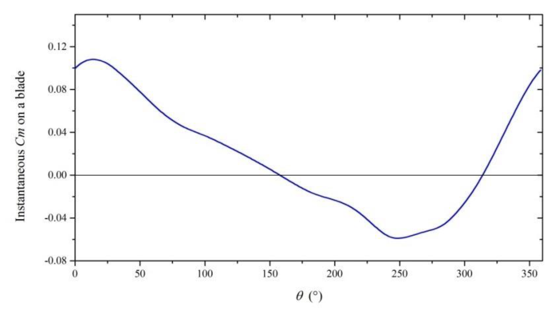
| Turbine Gap | Position at Cm = 0 |
|---|---|
| 0.75 D | 30.4° and 218.6° |
| 1.00 D | 25.8° and 218.3° |
| 1.50 D | 16.2° and 210.7° |
| 2.00 D | 7.40° and 201.5° |
| Wind Angle (°) | Maximum Cp | Optimal TSR | Wind Angle (°) | Maximum Cp | Optimal TSR |
|---|---|---|---|---|---|
| 0 | 0.0131 | 0.4 | 180 | 0.0625 | 0.8 |
| 22.5 | 0.1577 | 0.4 | 202.5 | 0.3469 | 0.8 |
| 45 | 0.4319 | 1 | 225 | 0.1025 | 0.6 |
| 67.5 | 0.8689 | 1.2 | 247.5 | 0.4042 | 0.4 |
| 90 | 0.6187 | 1.4 | 270 | 0.8692 | 1.4 |
| 112.5 | 0.3306 | 0.4 | 292.5 | 1.2093 | 1.4 |
| 135 | 0.1388 | 0.6 | 315 | 0.7489 | 1.6 |
| 157.5 | 0.3229 | 0.8 | 337.5 | 0.1844 | 0.4 |
© 2020 by the authors. Licensee MDPI, Basel, Switzerland. This article is an open access article distributed under the terms and conditions of the Creative Commons Attribution (CC BY) license (http://creativecommons.org/licenses/by/4.0/).
Share and Cite
Mao, Z.; Yang, G.; Zhang, T.; Tian, W. Aerodynamic Performance Analysis of a Building-Integrated Savonius Turbine. Energies 2020, 13, 2636. https://doi.org/10.3390/en13102636
Mao Z, Yang G, Zhang T, Tian W. Aerodynamic Performance Analysis of a Building-Integrated Savonius Turbine. Energies. 2020; 13(10):2636. https://doi.org/10.3390/en13102636
Chicago/Turabian StyleMao, Zhaoyong, Guangyong Yang, Tianqi Zhang, and Wenlong Tian. 2020. "Aerodynamic Performance Analysis of a Building-Integrated Savonius Turbine" Energies 13, no. 10: 2636. https://doi.org/10.3390/en13102636
APA StyleMao, Z., Yang, G., Zhang, T., & Tian, W. (2020). Aerodynamic Performance Analysis of a Building-Integrated Savonius Turbine. Energies, 13(10), 2636. https://doi.org/10.3390/en13102636