Wave Power Assessment in the Middle Part of the Southern Coast of Java Island

Abstract

An assessment of the wave power at the southern coast of the middle part of Java Island (Indonesia) was conducted based on a 15-year hindcast spectral wave model using the MIKE 21 Spectral Wave software. The model was forced with wind data with a 0.125° spatial interval and hourly time resolution. The obtained model was validated with field data collected from a buoy station that provided a set of significant wave height data with an hourly data interval for the whole month of June 2014. The validation showed that the obtained model matched the observed data with a minor average error. A spatial analysis was conducted in order to find the most suitable location for installing wave energy converters while taking into consideration the potential area demand, the wave power intensity, and the distance from the shore. Moreover, spatial analysis is conducted in order to find a suitable location to install wave energy converters, with consideration to potential area demand, wave power intensity, and distance from the shore. The best prospective location reached 30 kW/m of mean wave power intensity, 2.04 m of mean significant wave height, 8.9 s of mean wave period, 150 m of distance from the shoreline.

1. Introduction

Ocean wave energy has interested many researchers due to its high energy density [1,2] and contribution potential to the production of green electricity. It is estimated that 0.5 TW of power may be accessible from ocean waves [3]. The ocean wave energy conversion technique was first demonstrated and patented in 1799 by Girard and France [2]. Since then, various other techniques of converting ocean wave power into electricity have been developed [4,5].

The assessment of wave power potential is a necessary step in the process of installing wave energy converters (WECs), as it provides insights into the amount of energy that can be harnessed and also helps in selecting the optimal installation locations of the WECs. Accordingly, several spots have been analyzed, such as the east coast of peninsular Malaysia [6], the Korean Peninsula [7], the coast of Peru [8], the Mediterranean Sea [9,10,11], the Aegean Sea [2,10,12], Sicily (Italy) [13], the Australian coast [14,15], the coast of Spain [16], the coast of Portugal [17,18], the North Sea of Denmark [19], Santa Catarina (Brazil) [20], the Red Sea [21,22], the Black Sea [23], the Indian Ocean [24], and the Indonesian Sea [25,26]. These studies have used various wave models, such as the WAVEWATCH III [25], Simulating Wave Nearshore (SWAN) [16,17,23,27], WAve Model (WAM) [11,15,28], and MIKE 21 Spectral Wave (SW) [2,12,26] models.

In particular, Indonesia is fitted out with various large energy resources such as oil, gas, coal, geothermal resources, solar power, wind, and hydropower. According to [29], Indonesia was able to produce a total power of 44,000 MW in 2013, where most of the produced energy was from coal (44%). However, surprisingly, less than 5% of the produced energy was from renewable resources [30]. Unfortunately, this power is not enough to cover all the energy demands. Generally, the largest demand only comes from three islands: Java, Madura, and Bali, which consume about 80% of the total produced energy and only have 60% of the total population. According to the policies of the Indonesian government regarding the national energy sector, the primary energy consumption from renewable resources should be more than 23% by 2025 and 31% by 2050 [30,31].

According to [25,32,33,34,35], there is a lot of potential wave power around the Indonesian Sea, especially in the Indian Ocean at the west coast of Sumatra and the south coast of Bali, Nusa Tenggara Timur, Nusa Tenggara Barat, and Java. Unfortunately, until now, the spatial resolution of the provided areas that were assessed by these studies is not accurate enough. For example, the spatial resolution of the assessed area in [25] is 1°, as the data were retrieved from satellite observations (ENVISAT); therefore, it is very difficult to identify the optimal installation location for a WEC farm. Moreover, [25] only provided a two-year assessment of the wave power.

This study mainly focuses on the south coast of the middle section of Java Island (Central Java and Yogyakarta Provinces), which is in the Indian Ocean. In previous studies, the entire area of Indonesia was assessed without any particular focus on Java. In this study [25], our interest lies on the island of Java due to its high population of more than 100 million people, which amounts to one-third of Indonesia’s total population. In addition, our assessment was carried out with a better data resolution, which is eight times more accurate in comparison with the resolutions of the previous studies in [25]. Until now, no studies have been conducted using a high resolution to assess wave energy in Indonesia. Still, a high-resolution assessment is vital, as it makes it possible to obtain the specific coordinates of the optimum locations for the installation of WECs, where a high mean wave power intensity can be attained [36]. Moreover, other factors were considered in the selection of the prospective locations, such as the distance from the coast and the nearby population and industries. In this study, the spectral wave model was developed using the hindcast technique. In addition, the model was validated using the provided measurement data by the Agency for the Assessment and Application of Technology (BPPT).

The rest of the paper is organized as follows. The spectral wave model is presented in Section 2, the results are discussed in Section 3, and the conclusions are explained in Section 4.

2. Modeling

In this work, the MIKE 21 SW software was used for the wave hindcast and the subsequent evaluation of the wave climate at the studied coastal and offshore areas [37].

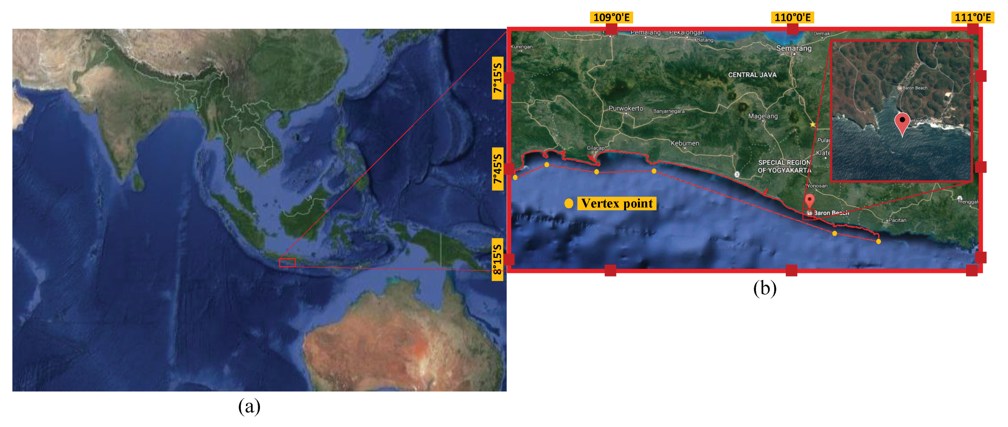
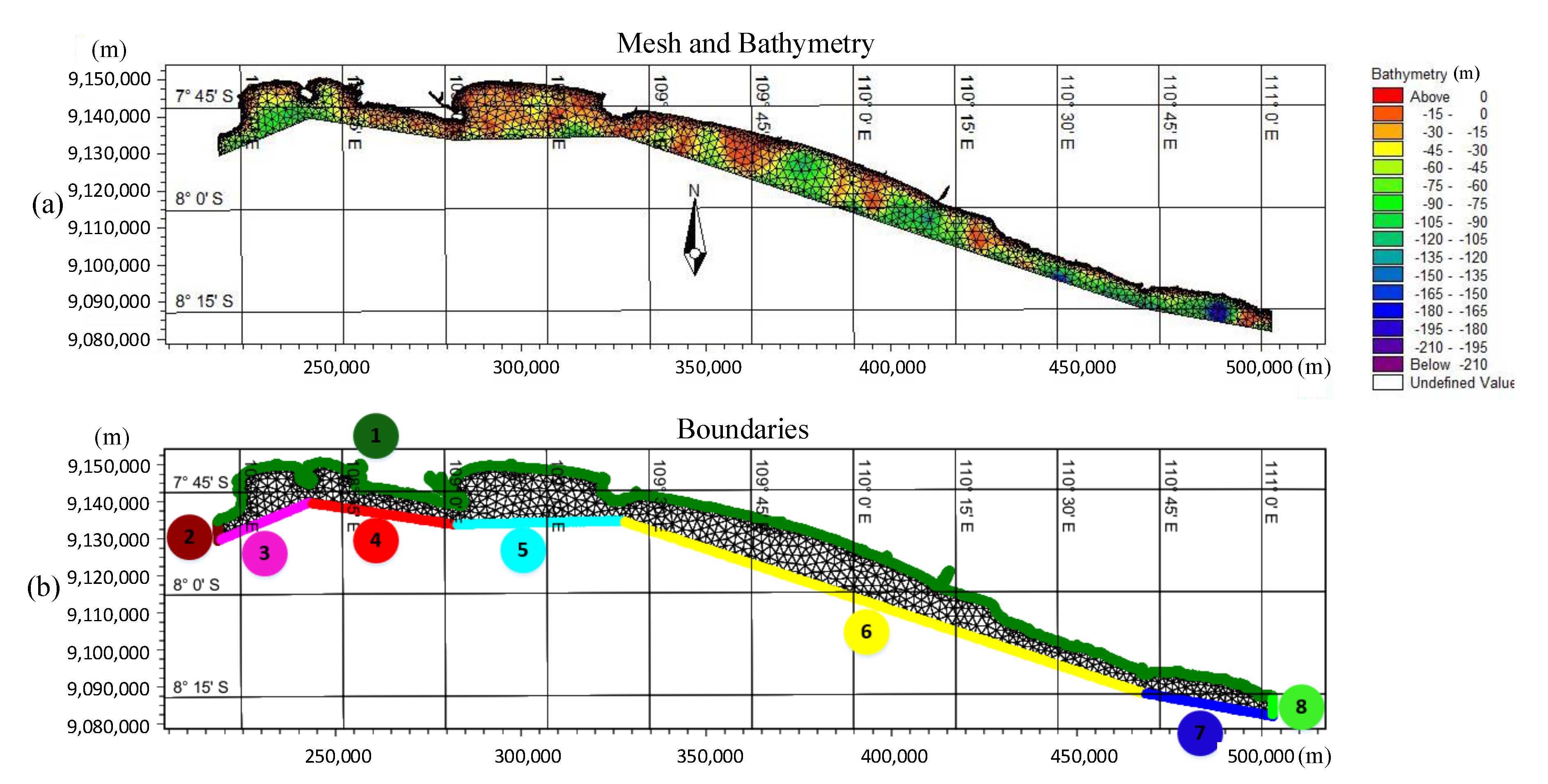
2.1. Simulation Domain

As mentioned above, the main areas of interest in this study are along the southern coastline of the central island of Java as shown in Figure 1a. The study area covers 108° E–112° E and 7° S–8° S and is approximately 3200 km². The coastline data were collected from a database of Global Self consistent, Hierarchical, High resolution Geography (GSHHG), which was maintained by the National Oceanic and Atmospheric Administration (NOAA) The coastline data were edited using the Geophysical Data System-Next Generation (GEODAS-NG), the Geographic Information System, and the MIKE Zero software. The simulation domain is shown in Figure 1b. The boundary of the study area was segmented into five straight lines, where the distance between each vertex point and the coastline is 5 km.

2.2. Data Collection and Model Setup

There are various types of raw data that can be used to build the model:

• Wind velocity, u and v components ($v_u$ and $v_v$),
• Significant wave height ($H_s$),
• Mean wave direction ($\theta$),
• Wave period (T),
• Bathymetry (h).

Items (1) to (4) were obtained from the European Centre for Medium-Range Weather Forecasts (ECMWF) [38]. The data have a spatial resolution of 0.125°. Thus, a further interpolation was necessary to feed the model with high-resolution data.

The simulation domain was discretized using the MIKE Zero Mesh Generator with the cell-centered finite element method, and the mesh was generated with unstructured triangular elements and 30 mesh smoothing iterations. The generated mesh is demonstrated by Figure 2, where it has 7537 elements and 4982 nodes with the mesh area between 1180 m² and 3,895,000 m². Furthermore, the bathymetry data were collected from the General Bathymetry Chart of the Ocean (GEBCO) with a spatial interval of 30-arc seconds, which is approximately equal to 1 km [39]. Subsequently, the bathymetry data were interpolated to each mesh node and element. Overall, this process provided a smoother bathymetry profile but obviously did not replicate any smaller-scale bottom features. Figure 2a shows the contour of the interpolated bathymetry data.

The boundary conditions are shown in Figure 2b. Mainly, in order to perform the computation, the boundary conditions have to be appropriately determined and correctly imposed. As shown in the figure, there are three types of boundary conditions used in this study: closed boundary (boundary 1), lateral boundary (boundaries 2 and 8), and wave parameter type 2 boundary (boundaries 3−7). The close or land boundary was applied for the coastline, which means that the water cannot flow across the boundary (no slips). The lateral boundary condition was set to the side lines where water can flow along the line (free slips). The wave parameter type 2 boundary was selected from the software with a format that varies in time along the line, and it requires four data types that are obtained from the ECMWF, which are the significant wave height, the wave period, the mean wave direction, and the directional standard deviation.

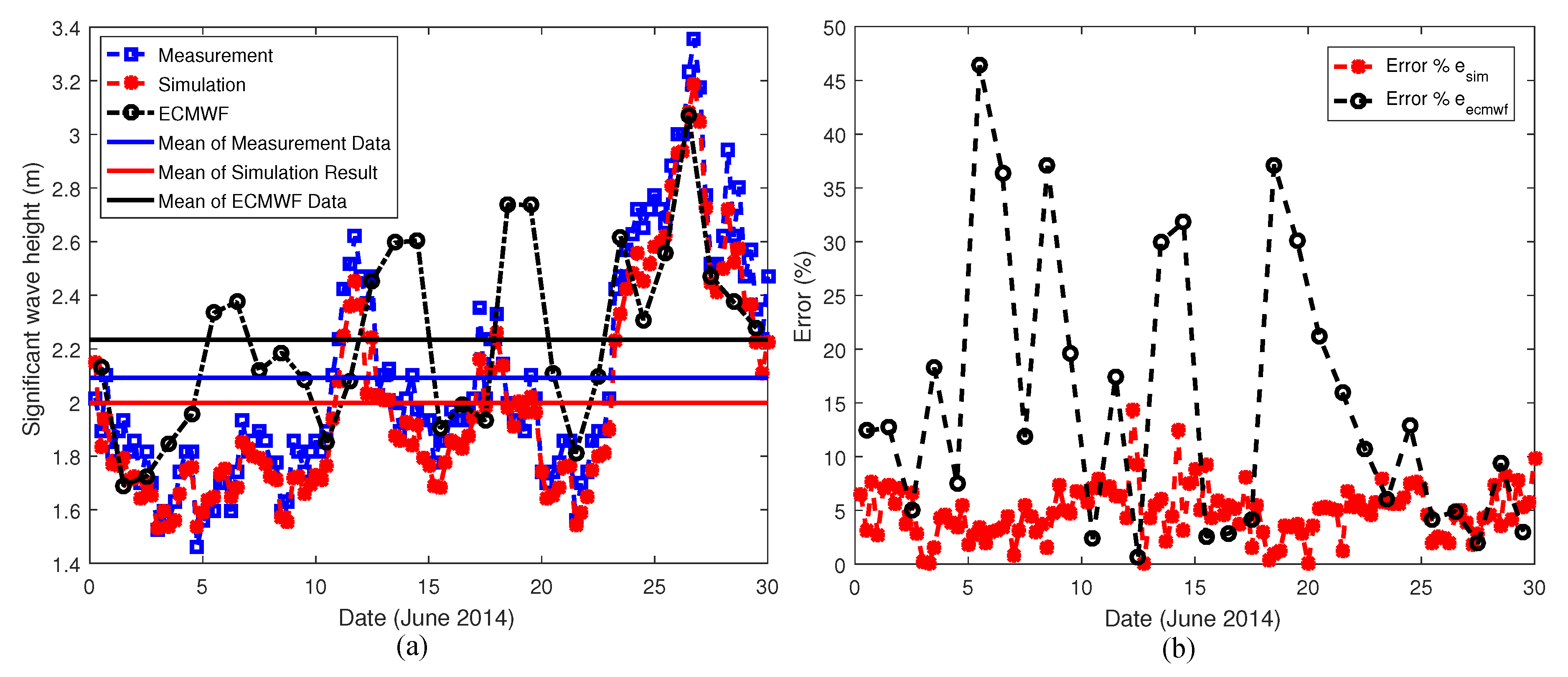
2.3. Model Validation

The validation of the spectral wave model is necessary in order to determine the accuracy of the proposed model. The objective of the validation process is to minimize the error between the simulated and the observed data by adjusting the parameters in the MIKE 21 SW software. The observed data were obtained from the buoy station, which is located at Baron Beach in the Central Java Province of Indonesia, 8.1364° S and 110.547° E. The station is operated by BPPT [40].

The spectral wave model in the MIKE 21 SW software was set using the listed parameters in

Table 1. Setting parameters of the spectral wave model in MIKE 21 SW.

Setting Parameter of the Spectral Wave Model in MIKE 21 SW			Setting Value
Spectral Discret.	Frequency discretization	Type	Logarithmic
		Number of frequency	25
		Minimum frequency	0.05
		Frequency factor	1.1
	Directional discretization	Type	360° rose
		Number or direction	16
Solution Technique	Instationary formulation	Geographical discretization	Higher order
		Maximum number of	32
		levels in transport calculation
		Number of step of source calc.	1
		Minimum time step	0.01 s
		Maximum time step	30 s
Wind forcing	Type	u and v components	DFS2 format
Energy forcing	Type	Quadruplet wave interaction	-
Wave Breaking	Breaking Coffesient ($\gamma$)	Constant	0.8
	Calibration constant ($\alpha$)	Constant	1
Bottom Friction	Nikuradse roughness ($k_N$)	Constant	0.04
White Capping	Dissipation coefficients	Constant	2 and 0.8
	($C_{dis}$ and $\delta$)

. The MIKE 21 SW software incorporates five different energy sources based on physical conditions. The energy sources phenomena were a wind input, a wave-wave interaction, a bottom friction, a a dept-induced breaking, and white capping. The dept-induced breaking source (or known as surf breaking source) was counted to accommodate waves propagation in shallow areas. According to [41,42], the dept-induced breaking source is formulated as

$$S_{surf}(f,\theta )=-\frac{2\alpha {\gamma }^{2}Q\overline{f}{d}^2}{H_{rms}^2}E(f,\theta )$$

(1)

where $S_{surf}$ is the shallow dept-induced breaking source, f is the frequency, $\theta$ is the wave approach direction, $\alpha$ is the calibration constant, $\gamma$ is breaking coefficient, Q is the fraction of breaking waves, $\overline{f}$ is the mean frequency, d is the water dept (shallow), $H_{rms}$ is the rms value of wave height, and E is the transported energy.

Furthermore, the white capping was also taken into account to accommodate the wave breaking that occurred in deeper water. Based on [41,43,44], the white captain energy source is formulated as

$$S_{wc}(f,\theta )=-C_{ds}{\left(\frac{\widehat{\alpha }}{\widehat{{\alpha }_{PM}}}\right)}^m\left[(1-\delta )\frac{k}{\overline{k}}+\delta {\left(\frac{k}{\overline{k}}\right)}^2\right]\overline{\sigma }E(f,\theta )$$

(2)

where $S_{wc}$ is the white capping energy source, $\widehat{\alpha }$ is wave field for the overall spectrum, $\widehat{{\alpha }_{PM}}$ are the wave field for the Pierson–Moskowitz spectrum, m is the fitting parameters, $\overline{\sigma }$ is the mean relative angular frequency. The constants k and $\overline{k}$ are the wave number and its mean value, respectively. The parameters of $C_{ds}$ and $\delta$ are the dissipation coefficients.

The validation process was deployed to decide whether the setting parameters are acceptable or not. Figure 3a shows a comparison between the measured, simulated, and ECMWF data of the significant wave height in June 2014. As seen in the figure, there is only a small absolute error between the measured and the simulated data ($e_{sim}$). The maximum value of $e_{sim}$ is 0.34 m, with an average error of about 5 %, which indicates that the model is acceptable and ready for use in the hindcasting simulation. Meanwhile, the absolute error between the measured and the ECMWF data ($e_{ecmwf}$) is bigger in comparison with that of $e_{sim}$, as it has an average value of 15 %. This indicates that the ECMWF data cannot be used alone to assess the wave characteristics. Furthermore, the spatial resolution from the ECMWF is not small enough to determine a prospective location for a WEC farm.

In this study, the wave power was calculated using the following equation [12,16,36,45]:

$$P=\rho g{\int }_0^{2\pi }{\int }_0^{\infty }{C}_g(f,\theta )E(f,\theta )dfd\theta$$

(3)

where P is the wave power per unit width, $\rho$ is the water density, g is the acceleration due to gravity, $C_g$ is the wave group velocity, E is the transported energy, f is the frequency, and $\theta$ is the wave approach direction. According to Figure 2, the water depth in the study area is in the range of shallow to intermediate. Therefore, it is important to apply appropriate wave group velocities [36], which are in this case formulated as

$$C_g=\sqrt{gh}$$

(4)

for shallow water, and

$$C_g=\frac{\omega }{2k}\left(1+\frac{2kh}{sinh\left(2kh\right)}\right)$$

(5)

for intermediate-depth water, where $\omega =\sqrt{gktanh\left(kh\right)}$ is the wave dispersion relation, h is the water depth, k is the wave number equal to $2\pi /\lambda$, and $\lambda$ is the wave length.

3. Results and Discussion

Several variables were analyzed in this study, such as the mean wave power intensity ($\overline{P}$), the mean wave period ($\overline{T}$), and the mean significant wave height (${\overline{H}}_s$). To make the data analysis easier, the simulations were separated into 15 running steps. The simulation results and analyses are discussed below.

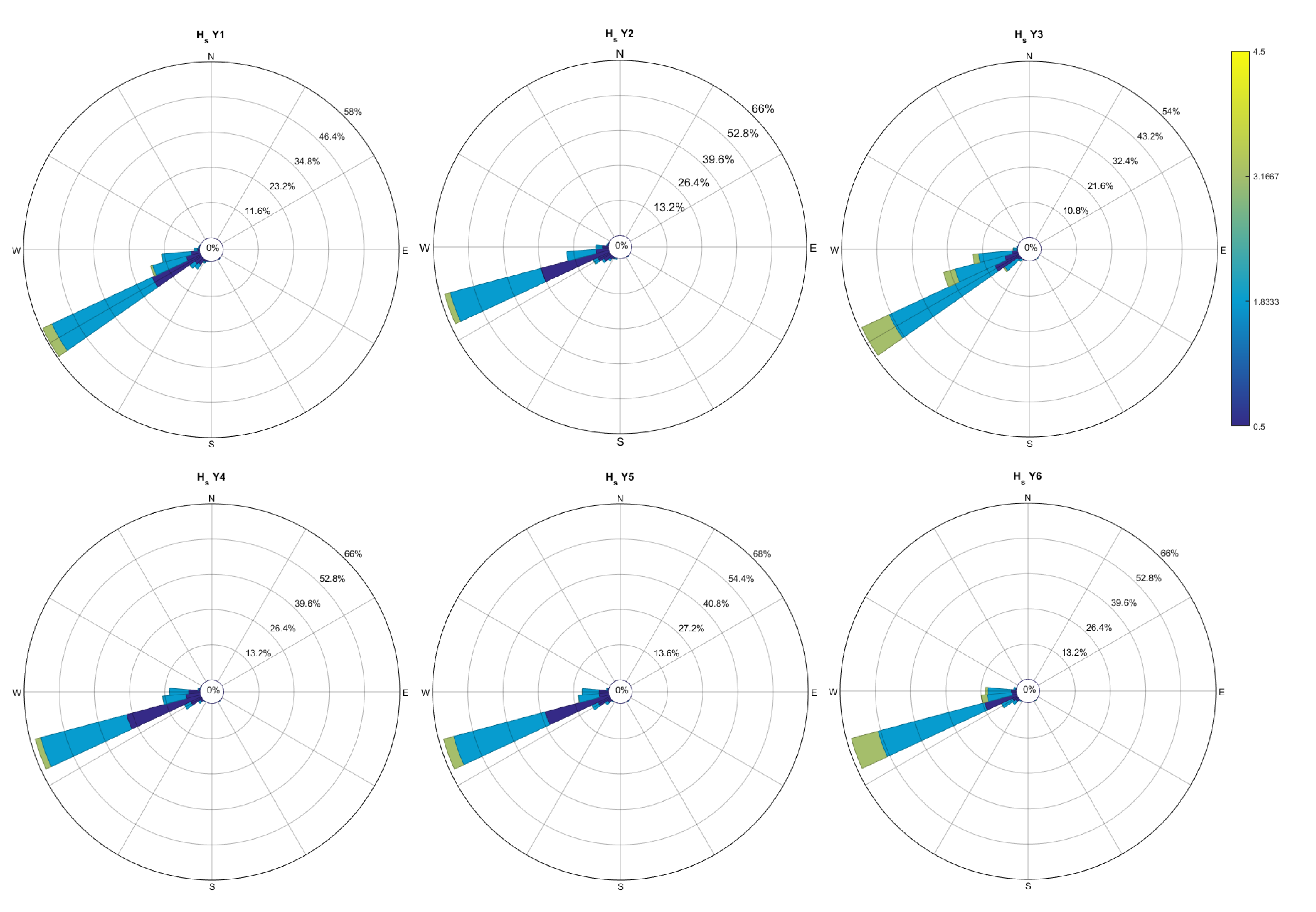
3.1. Time-Domain Analysis

A time-domain analysis is necessary because it provides the evolution of the wave parameters over time and enables the determination of the wave power level for a specific duration. The results are discussed in the following subsections.

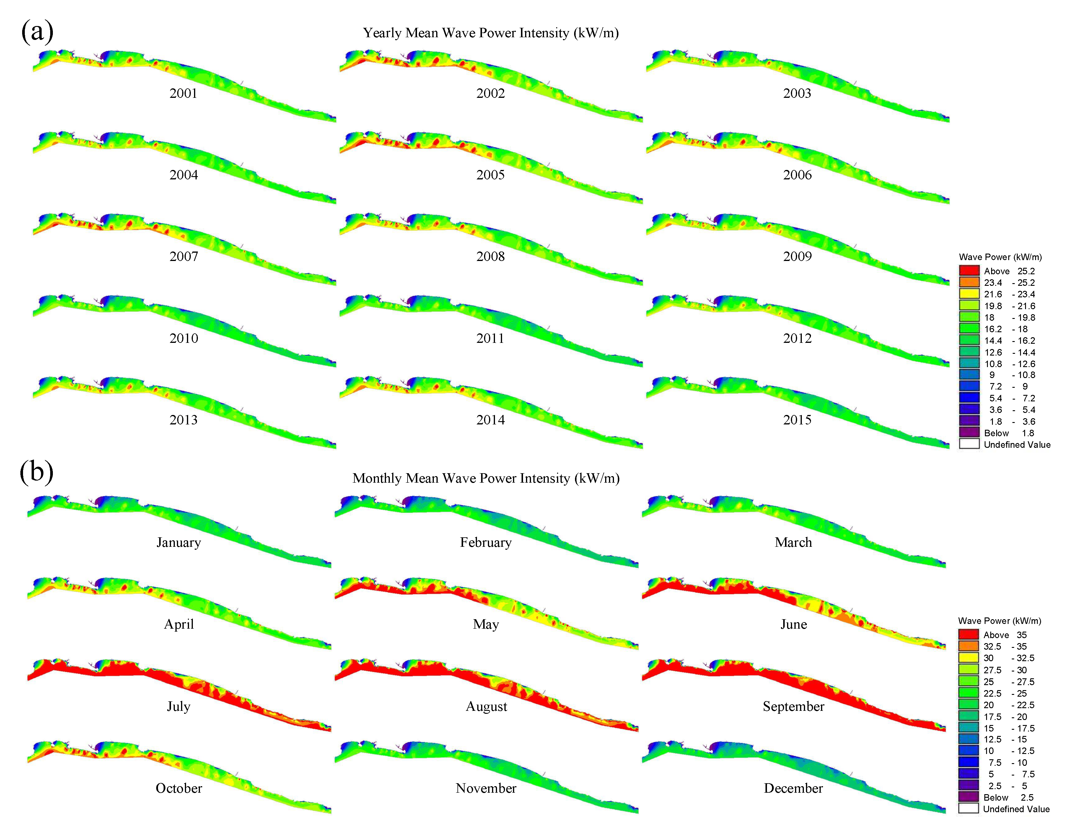
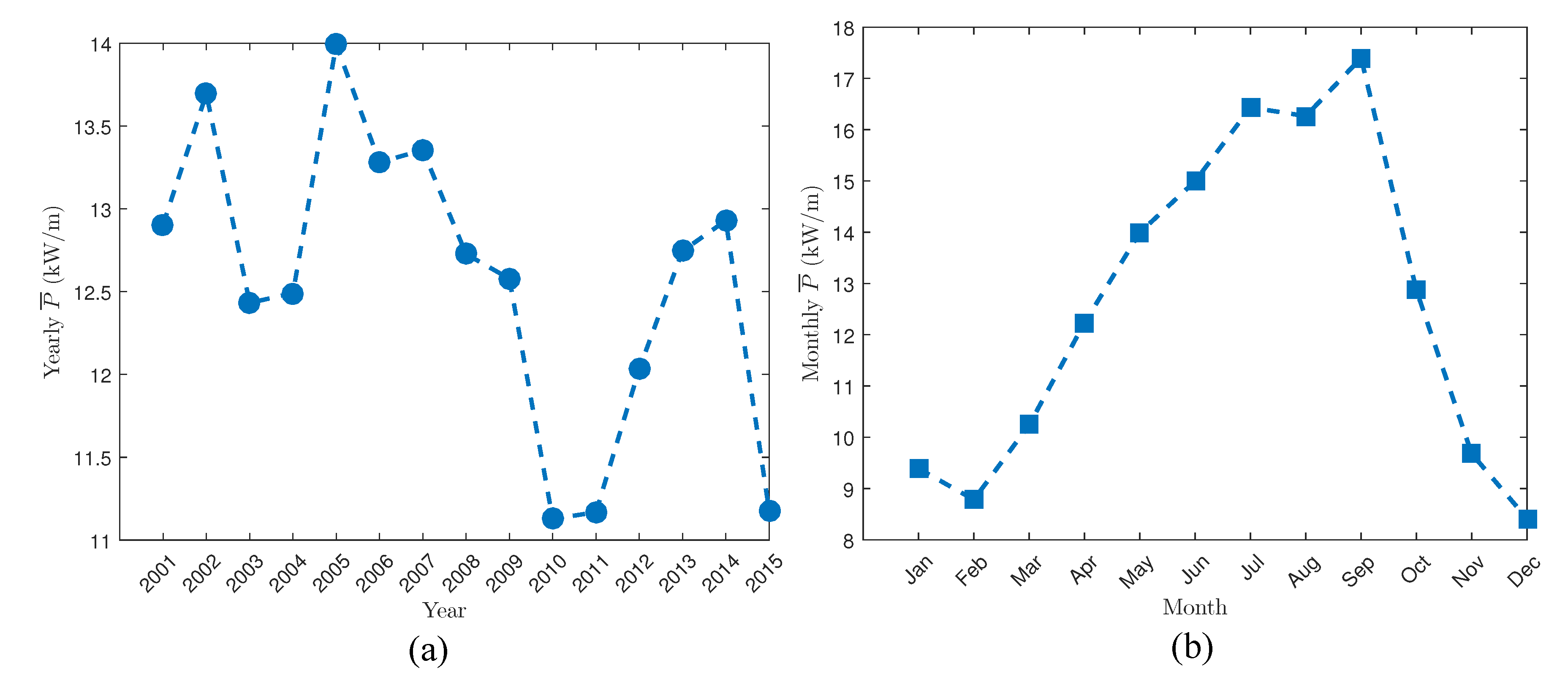
3.1.1. Yearly Analysis

An annual analysis was conducted using the time-average value for each year, and Figure 4a shows the distribution of the yearly mean wave power from January to December. There are minor fluctuations in the mean wave power intensity from year to year. Figure 5a shows the time evolution of the average power from all the elements. It can be seen that the fluctuation is in between 10 and 13 kW/m, where the highest value occurred in 2005 with a value of 14 kW/m, and the lowest value occurred in 2010 and did not exceed 11.1 kW/m. This indicates that the mean wave power intensity is quite stable over the years.

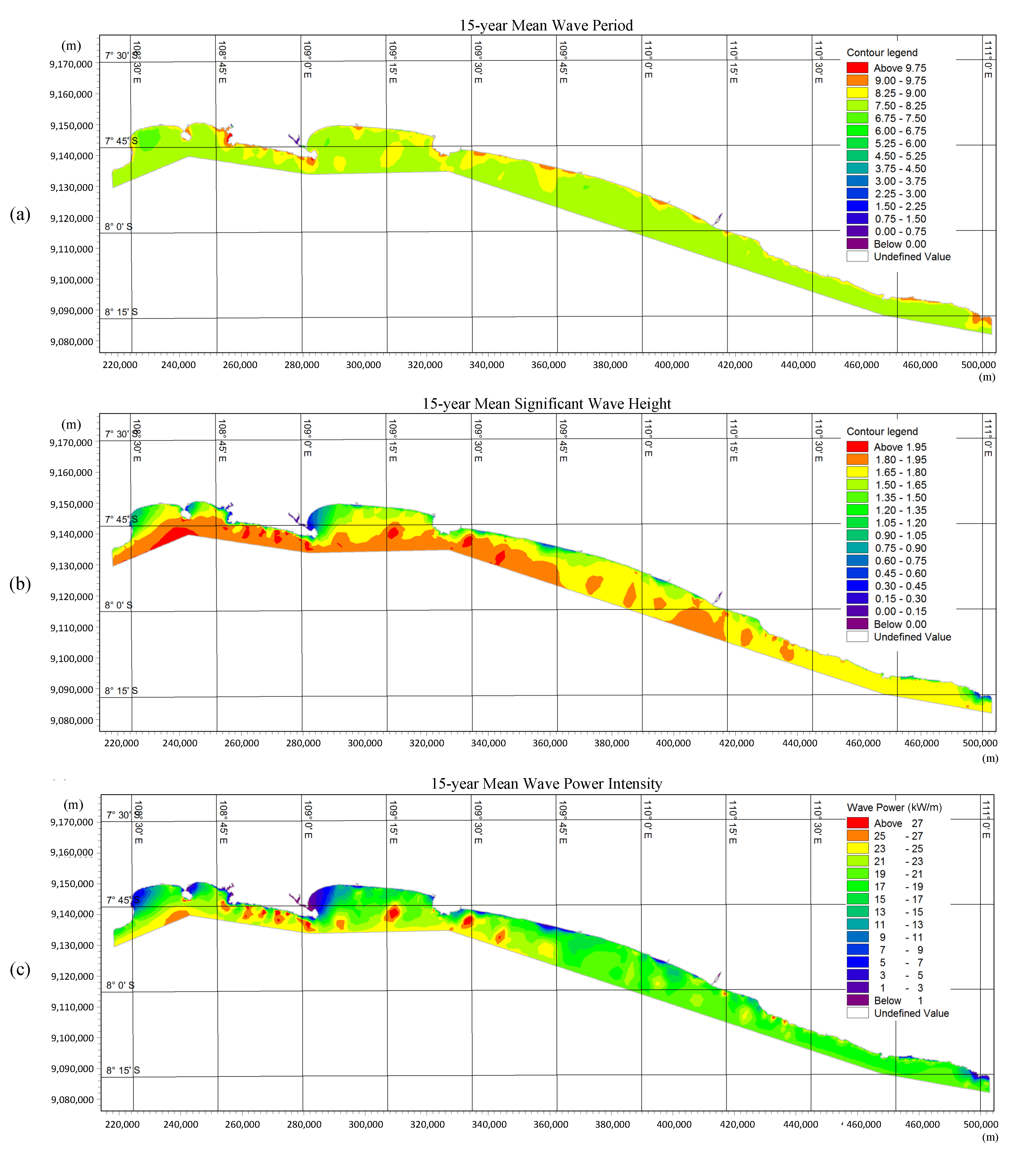
3.1.2. 15-Year Mean Analysis

This analysis was conducted by time-averaging from the entire 15-year assessment duration for each mesh element. Figure 6a shows the distribution of the 15-year mean wave period ($\overline{T}$), where the maximum and average values are 10.1 s and of 7.9 s, respectively, and Figure 6b shows the contour of the 15-year mean significant wave height, where the maximum and average values are 2.2 m and 1.2 m, respectively. Furthermore, the mean wave power intensity parameter is shown in Figure 6c, and its average and maximum values are 12.6 kW/m and 36.9 kW/m, respectively.

3.1.3. Monthly Analysis

A monthly analysis was conducted to show the wave power intensity for each month and identify the periods when the intensity was high and low. The analysis was made by taking the time-average value from the 15-year hindcast for each month. Figure 4b shows the contour of the mean wave power intensity for each month. From July to September, most of the locations had a high mean wave power intensity as shown in red. Figure 5b shows the average of the monthly mean wave power intensity for each month. The three highest values are 17.4 kW/m, 16.4 kW/m, and 16.3 kW/m, and they were recorded in the months of September, July, and August, respectively. During these months, this region usually experiences strong monsoon wind from the direction of Indian Ocean. It certainly brings up the sea level during this season. Meanwhile, the lowest mean wave power intensity values took place in the months of December, January, and February during the rainy season, with values of 8.4 kW/m, 9.4 kW/m, and 8.8 kW/m, respectively.

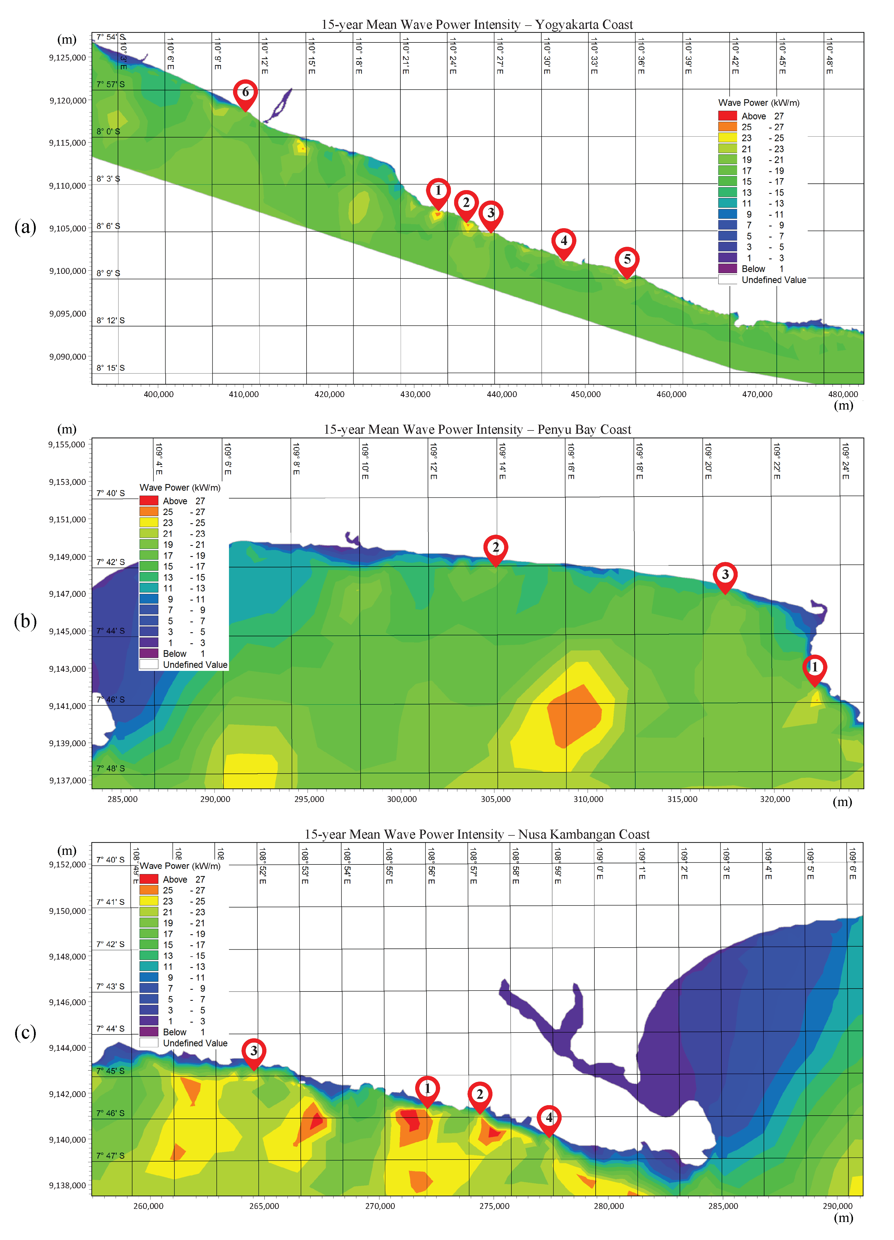
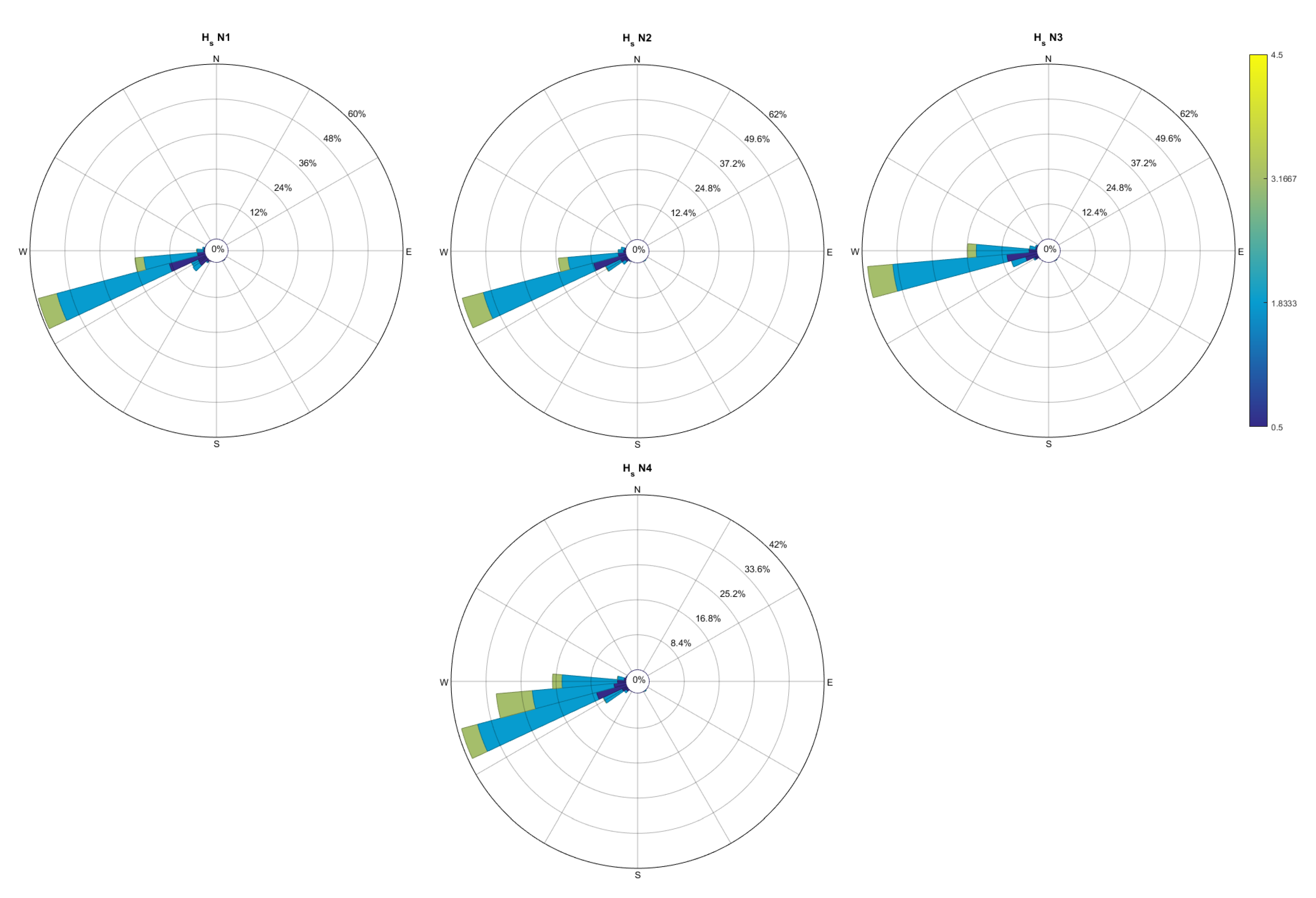
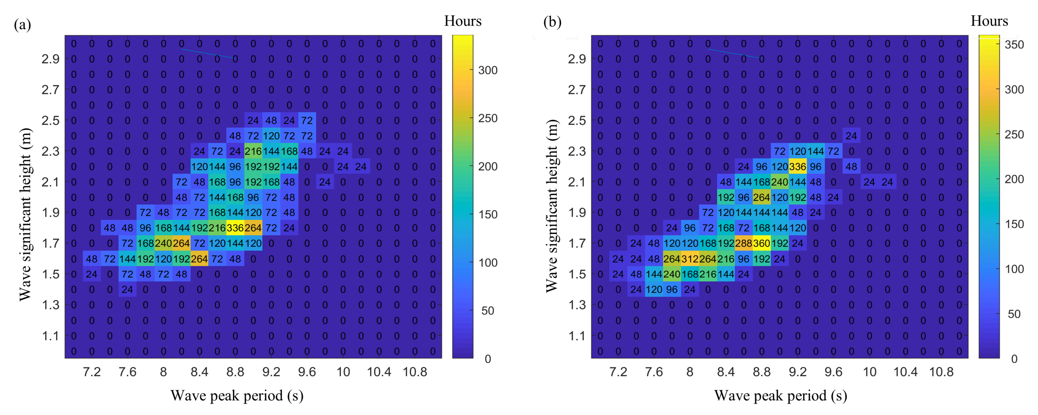
3.2. Spatial Analysis

An analysis in the space domain was conducted in order to determine the prospective locations for the installation of WECs. There are several parameters entailed in determining the suitable prospective locations, such as $\overline{T}$, $\overline{H_s}$, $\overline{P}$, distance to the land/coast (d), water depth (h), and potential demand. The d parameter is important due to its direct relation to the production, operation, and distribution costs. The potential demand is observed by considering nearby situations, such as the population and the industrial conditions and activities. In this study, three discrete regions were analyzed: Yogyakarta, Penyu Bay, and Nusa Kambangan coasts.

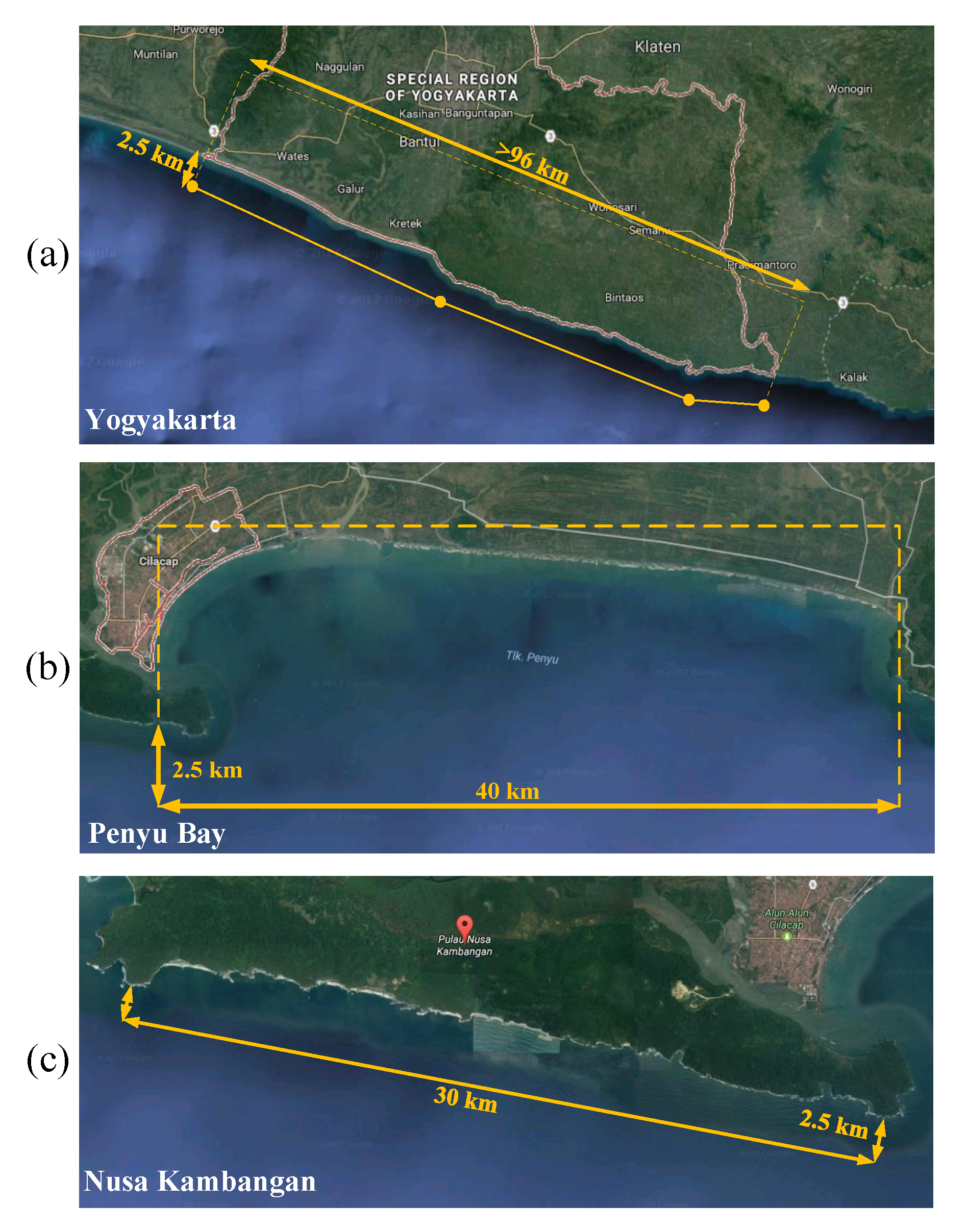
3.2.1. Yogyakarta Coast

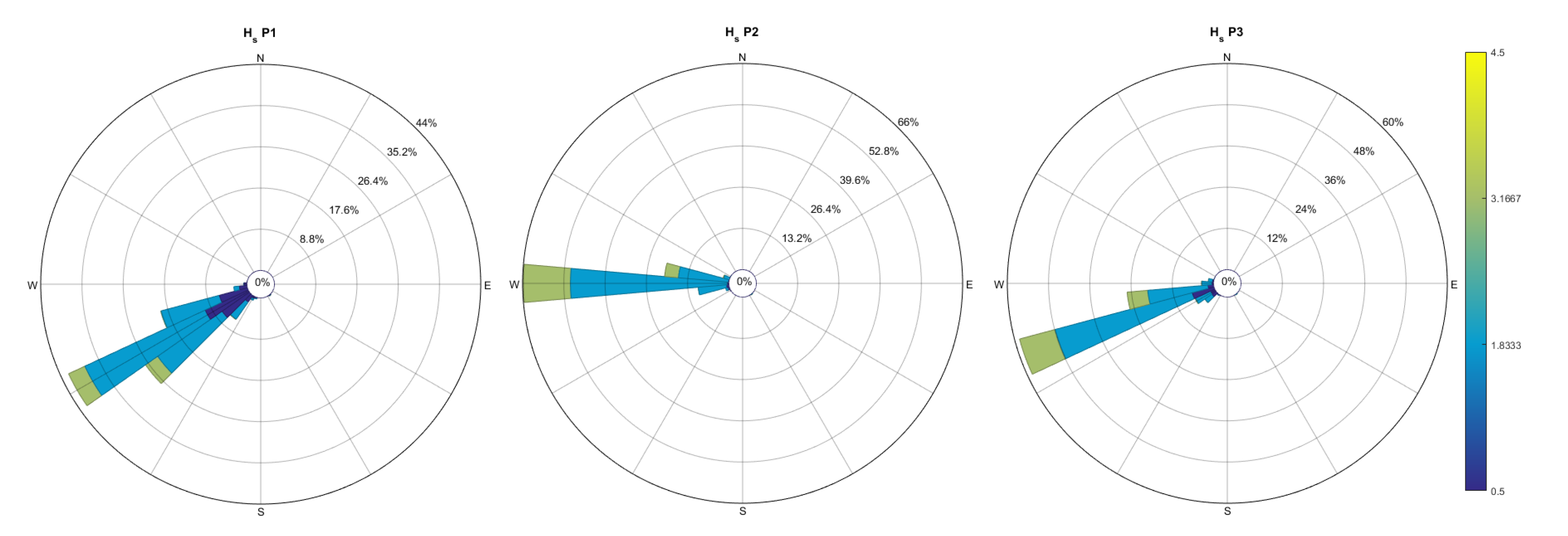
The special Region of Yogyakarta is an Indonesian province with a high population density. In 2015, the total population in Yogyakarta was around 3.7 million, with a density of more than 1000 people/km², and it keeps growing every year. In 2012, it was reported that Yogyakarta had 391 industries in various sectors, such as the manufacturing of computers and electronics, foods and beverages, textiles, leather products, wood products, chemicals, pharmaceuticals, refined oil products, and other industries. Yogyakarta is known as one of the more developed regions, and it also has a high economic growth rate. In 2015, the economy of Yogyakarta grew by approximately 5%, which indicates that the demand for energy and electricity in this region is relatively high in comparison with other regions.

Furthermore, Figure 7a shows a map of the beaches along more than 96 km of the coastline of Yogyakarta. The analysis is limited to a range of 2.5 km wide. The distribution of the mean wave power intensity for the 15-year assessment is shown in Figure 8a.

As shown in Figure 8a, six locations were selected as prospective and suitable locations for the installation of WEC farms, and their detailed coordinates are listed in

Table 2. Prospective WEC locations with the estimated mean wave power based on the 15-year assessment along the Yogyakarta, Penyu Bay, and Nusa Kambangan coasts.

Location	Latitude (°S)	Longitude (°E)	$\overline{\mathit{P}}$ (kW/m)	${\overline{\mathit{H}}}_{\mathit{s}}$ (m)	$\overline{\mathit{T}}$ (s)	d (m)	h (m)
Yogyakarta Coast
1	8.079190	110.390709	30	2.0	8.9	150	35
2	8.090876	110.424812	30	2.0	9.1	250	55
3	8.101757	110.439587	27	2.0	8.9	150	30
4	8.131859	110.522797	24.8	1.9	8.6	125	30
5	8.146277	110.582598	24.8	1.9	8.9	175	22
6	7.972976	110.184429	22.5	1.8	8.8	200	22
Penyu Bay Coast
1	7.758631	109.386500	25.5	1.9	8.8	200	72
2	7.699657	109.230078	22.5	1.8	8.8	400	10
3	7.715494	109.344885	21	1.6	8.8	550	18
Nusa Kambangan Coast
1	7.762734	108.933951	27.5	2.0	9.2	250	26
2	7.765251	108.953376	27	2.0	8.9	200	36
3	7.747749	108.865256	27	2.0	9.0	250	23

. It can be seen that the most suitable location has a mean wave power intensity of more than 30 kW/m, a mean significant wave height of 2.1 m, and a mean wave period of 8.9 s. Additionally, this location is very close to the coast, as it is only less than 150 m away from the coastline. The second prospective location has the same mean wave power intensity as the first one, but it is located at a farther distance from the coast (250 m). The sixth prospective location has a mean wave power intensity of 22.5 kW/m and a mean significant wave height of 1.8 m, and it is less than 200 m away from the coast. The polar diagrams of the yearly significant wave height for the prospective locations in Yogyakarta coast are shown in Figure 9.

3.2.2. Penyu Bay

Penyu Bay is located next to the Cilacap Regency in the Central Java Province. Based on the population density report from the Statistics Centre Department, as of 2014, Cilacap is the largest area and the most populated regency in the Central Java Province. The total population was more than 1.6 million people with a population density of approximately 788 people/km². Additionally, Cilacap is home to various industries, including fish processing, oil refining, and cement production.

The map of the study area in Penyu Bay is shown in Figure 7b. The area has a span of 44 km and a width of 2.5 km (measured from the farthest coastal point). Figure 8b shows the contour of the mean wave power intensity distribution at the Penyu Bay area and its three prospective locations. Table 2 shows the details of the three-point prospective locations. The mean wave power intensity reached 25.5 kW/m, 22.5 kW/m, and 21 kW/m for the first, second, and third prospective locations, respectively. The distance of the third prospective location is quite large (550 m). The polar diagrams of the yearly significant wave height for the prospective locations in Penyu Bay coast are shown in Figure 10.

3.2.3. Nusa Kambangan Coast

Nusa Kambangan is an island separated from the island of Java by a narrow strait. Administratively, however, it belongs to the Central Java Province. The island is mostly used as a location for Indonesia’s national prisons, and it is close to the Cilacap Regency as shown in Figure 7c. The considered area in the analysis is limited to a range of a width of 2.5 km and an approximate span of 28 km. Surprisingly, there are three locations where the mean wave power intensity reached 27 and 27.5 kW/m, as shown in Table 2. The mean wave power intensity distribution is presented in Figure 8c. The polar diagrams of the yearly significant wave height for the prospective locations in Nusa Kambangan coast are shown in Figure 11.

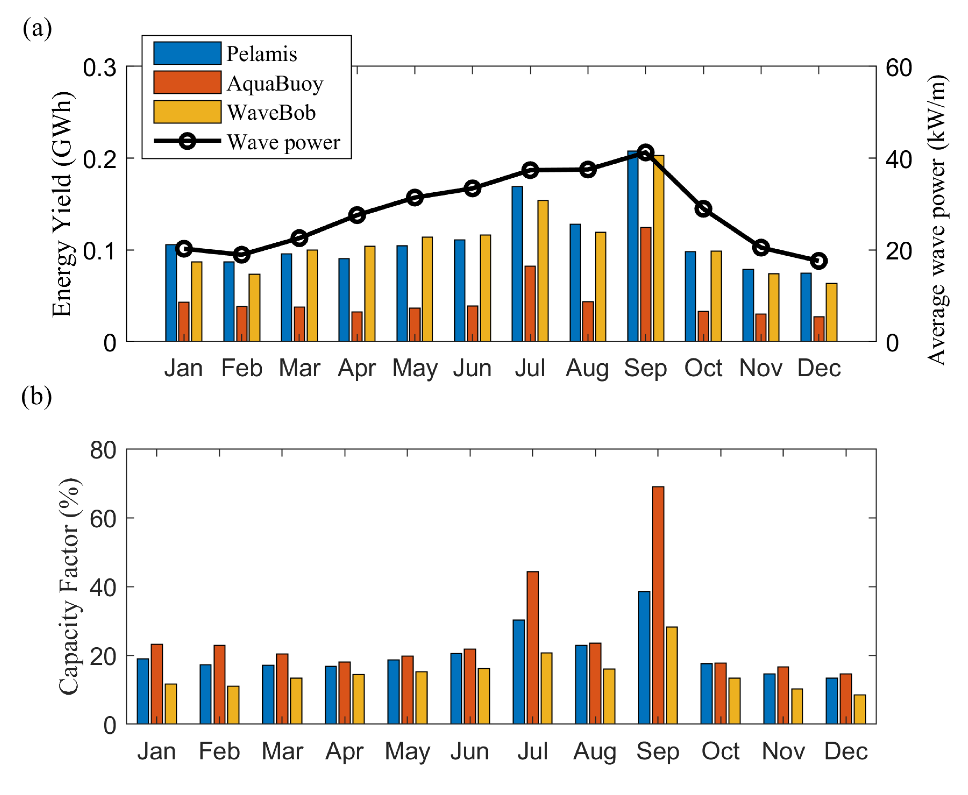
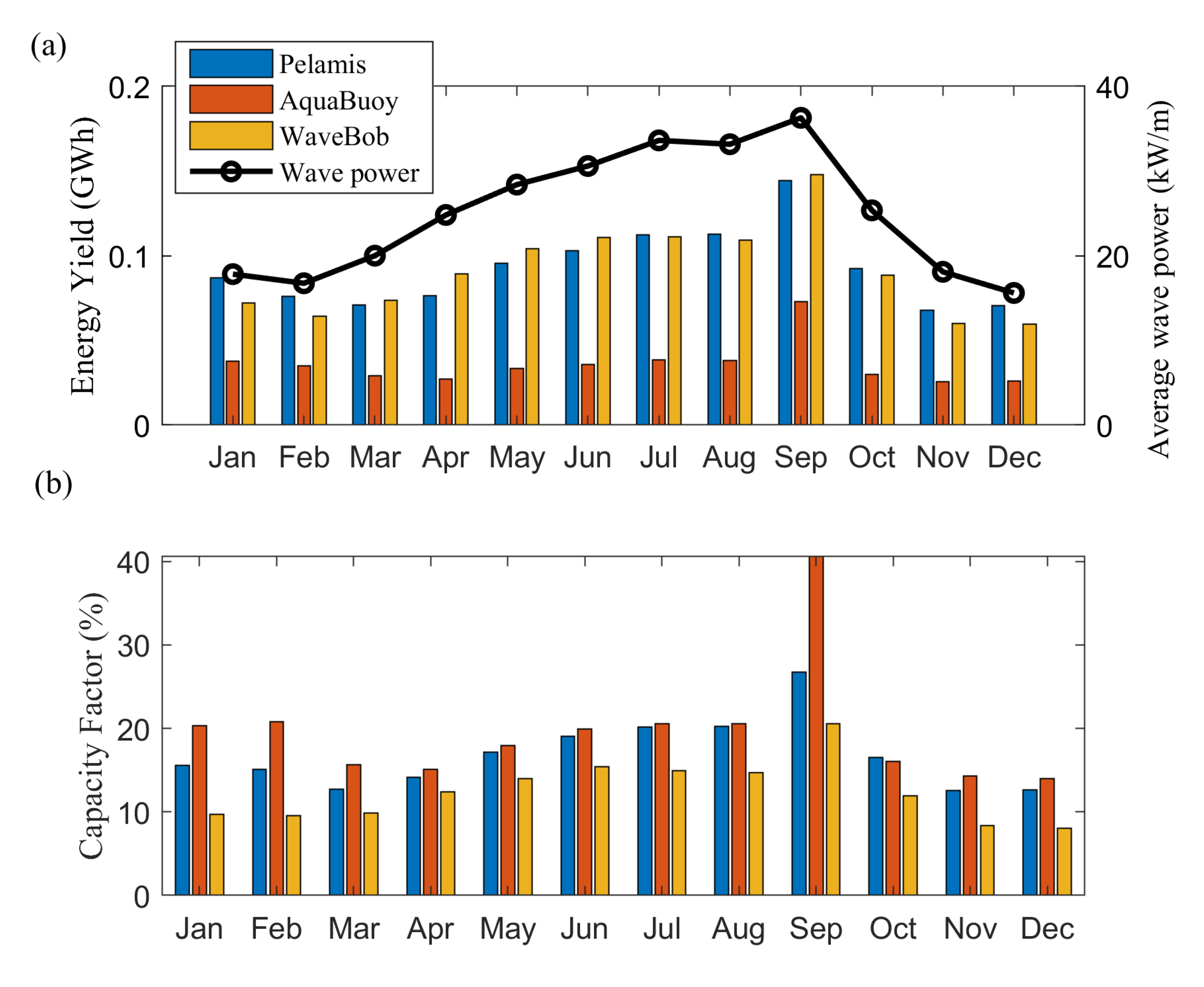
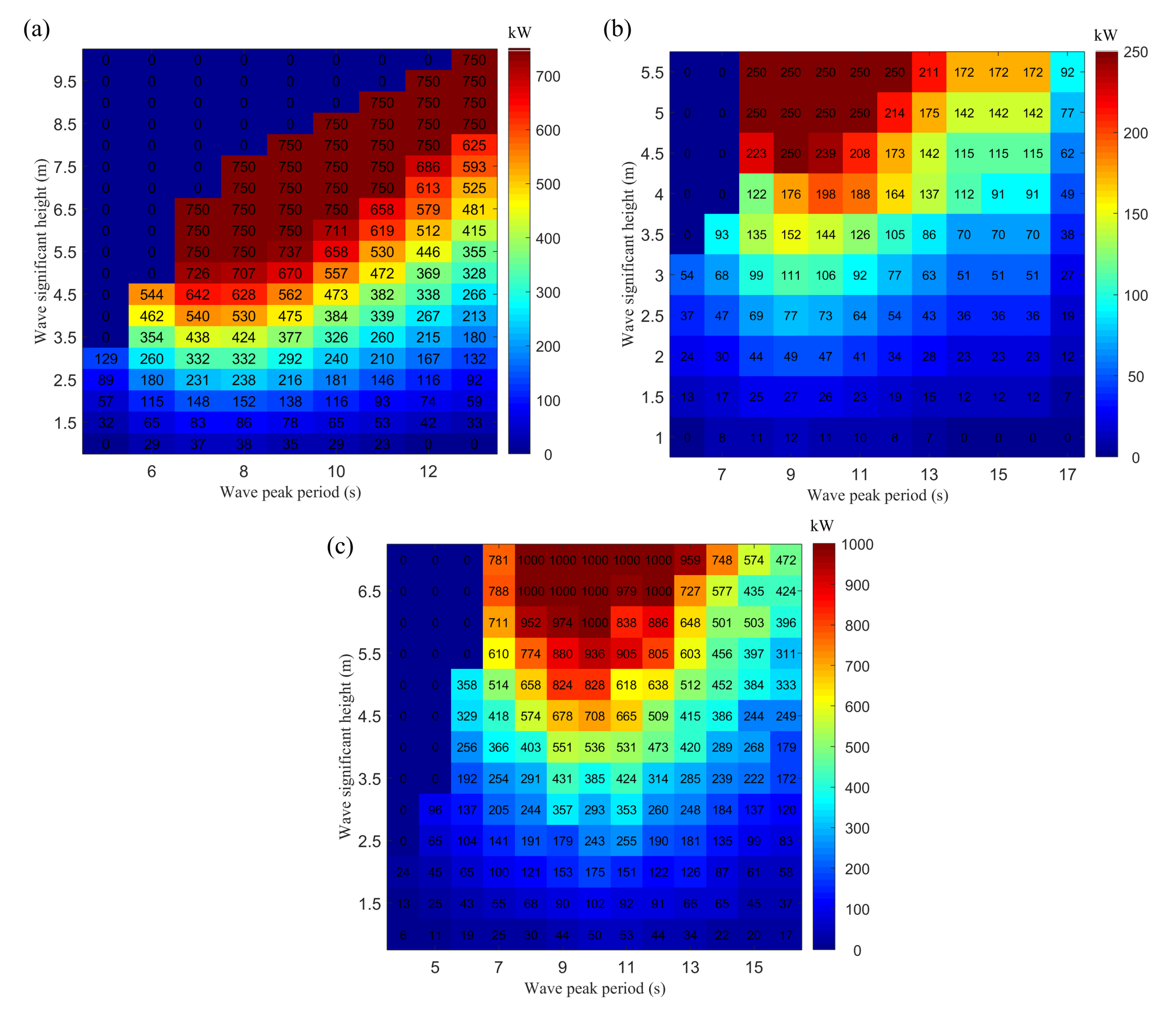
3.3. Wave Energy Generation

To further investigate the spots selected as potential locations for wave energy harvesting, the performance of known wave energy conversion devices subject to the wave conditions in two sites off the coast of Yogyakarta and Penyu Bay, was examined. The wave energy conversion technologies used in this work are:

• The Pelamis is an offshore semi-submerged slack-moored wave energy converter. The device is made of floating cylinders interconnected through hinged sections. The relative wave-induced motion of the cylinders against each other is converted to useful electricity via the hydraulic power take-off (PTO) system placed in the hinged sections [46]. The full scale version of the Pelamis, with rated power of 750 kW, is used in this study. The power matrix of the device is shown in Figure 12a.
• The AquaBuoy is an offshore semi-submerged heaving wave energy converter. The vertical wave-induced motion of the buoy is utilized to pump the sea water into a Pelton turbine, which in turn drives an electric generator [47]. the nameplate power rating of the device is 250 kW and the corresponding power matrix is shown in Figure 12b.
• The Wavebob is an offshore two-body heaving wave energy converter. The relative motion between the floating body and the submerged body is utilized to generate electricity through hydraulic direct-drive PTO system [48]. The full scale version of the Wavebob WEC used in this study is 1000 kW as indicated in the device power matrix depicted in Figure 12c.

Due to the fact that the selected WEC technologies are designed to operate at sea depths greater than 50 m, only two sites out of twelve potential sites have the needed sea depths as shown in Table 2 [49]. The first site is location 2 off the coast of Yogyakarta, while the other is location 1 off the coast of Penyu Bay. Both sites have an annual average wave power intensity of 30 kW/m and 25.5 kW/m, respectively. The selected sites are located at a distance not more than 250 m from the coastlines. The wave resource potential can be represented using wave scatter diagram, in which the wave occurrences in hours are counted based on the wave significant height and peak period data obtained from the 15-year wave hindcast simulation conducted in Section 2. The wave scatter diagrams of the two selected sites are depicted in Figure 13. It is obvious that the first site (location 2 in Yogyakarta) has more wave resource than site 2 (location 1 in Penyu Bay), where the occurrences of the waves with significant heights greater than 2 m in the first site is 30% more than that of the second site (location 1 in Penyu Bay).

The average annual energy yield (AEY) of the three adopted WEC technologies is computed through multiplying the devices power matrices by the wave scatter diagrams, then the generated energy at all wave bins are summed. Similarly, the average monthly energy yield (MEY) is calculated through overlaying the devices power matrices and the monthly wave scatter diagrams of the selected sites. Another metric that assesses the WEC technology profitability is the device capacity factor (CF), which is the ratio of the device generated energy and the rated generated energy (using the device rated power). The higher the average CF, the more often the WEC operates closer to its nameplate capacity, which makes the system economically viable.

For the first site (location 2 Yogyakarta), the Pelamis produced the highest average AEY, 1.35 GWh, which is approximately 5% greater than the average AEY of the Wavebob and almost 60% greater than the average AEY of the AquaBuoy. These results agrees with the fact that both the Pelamis and Wavebob are significantly greater in power rating compared to the AquaBuoy. The Pelamis slightly outperformed the Wavebob, even though its power rating is 25% lower than that of the Wavebob. This is due to the fact that the Pelamis has better wave-to-wire efficiency at low wave power intensities as shown in Figure 12. As for the average capacity factor (CF), the Aquabuoy has the highest average CF, 25%, compared to 20% and 14% recorded for the Pelamis and Wavebob, respectively. The recorded average AEY values are noticeably lower at the second site (location 1 Penyu Bay), and thats due to the lower wave resource compared to the first site. Again the Pelamis outperformed the other two WEC devices producing an average AEY of 1.11 GWh, whereas the AquaBuoy and Wavebob WECs managed to produce 0.43 GWh and 1.10 GWh, respectively. The corresponding average CF values at the second site ranges from 12% for the Wavebob to 20% for the AquaBuoy. The average monthly energy yield (MEY) distribution at both sites show a strong correlation with the average monthly wave power intensity distribution. Higher MEY values are observed for July, August, and September, while relatively lower values are recorded during winter months. The Pelamis and Wavebob WECs produced superior average MEY values compared to the smaller AquaBuoy WEC across all months as shown in Figure 14a and Figure 15a. The AquaBuoy WEC has the highest average monthly CF values for both sites, especially in September, in which the CF of the device reached 60% and 40% for the first and second sites, respectively (see Figure 14b and Figure 15b). Having greater power rating does not necessary ensure superior performance, this was the case with the Wavebob WEC which failed to outperform the Pelamis in both sites as shown in Figure 14a and Figure 15a.

4. Conclusions

The Indian Ocean wave characteristics were simulated for the south coast of the middle section of Java Island. A 15-year duration hindcast simulation was carried out using the MIKE 21 SW software, which was developed by DHI. The model parameters were validated using a one-month period with an hourly measurement interval according to the data recorded by the buoy station, which is located at Baron Beach on the coast of Yogyakarta. The validation showed an approximate minor average error of 5%.

According to the time-domain analysis, the maximum mean significant wave height was 2.2 m, with an approximate average value of 1.2 m. The maximum mean wave period was 10.1 s, with an approximate average value of 7.8 s. The maximum and average mean wave power intensity values are 36.9 kW/m and 11.6 kW/m, respectively. These values indicate a great amount of potential power. The monthly analysis showed that during the months of July, August, and September, the mean wave power intensity reached its peak value, which exceeded 16 kW/m. However, the peaks of the mean wave power intensity for the months of December, January, and February were below 10 kW/m. Based on the annual analysis, the mean wave power intensity varied between 11.1 kW/m and 14 kW/m.

A spatial analysis of the Yogyakarta, Penyu Bay, and Nusa Kambangan coasts was conducted. The results resulted in a total of 12 likely prospective locations suitable for the installation of WEC farms. Six points were found along the coast of Yogyakarta, with the best prospective location (8.079190° S and 110.390709° E) having a mean wave power intensity of 30 kW/m, a mean significant wave height of 2.04 m, a mean wave period of 8.9 s, and a distance of 150 m from the shoreline. Along the coast of Penyu Bay, three prospective locations were found, with the best prospective location (7.758631° S and 109.3865° E) having a mean wave power intensity of 25.5 kW/m, a mean significant wave height of 1.9 m, a mean wave period of 8.8 s, and a distance of 200 m from the shoreline. Along the coast of Nusa Kambangan, three prospective locations were found, with the best prospective location (7.762734° S and 108.933951° E) having a mean wave power intensity of 27.5 kW/m, a mean significant wave height of 2.0 m, a mean wave period of 9.2 s, and a distance of 250 m from the shoreline. Three different WEC technologies were tested at two potential sites off the coasts of Yogyakarta and Penyu Bay. The WEC technologies were analyzed and compared based on their annual and monthly energy yield and device capacity factor. The Pelamis proved to produce the highest energy yield, while preserving a good average capacity factor.

References

1. Clement, A.; McCullen, P.; Falcao, A.; Fiorentino, A.; Gardner, F.; Hammarlund, K.; Lemonisa, G.; Lewish, T.; Nielseni, K.; Petroncinij, S.; et al. Wave energy in Europe: Current status and perspectives. Renew. Sustain. Energy Rev. 2002, 6, 405–431. [Google Scholar] [CrossRef]
2. Jadidoleslam, N.; Ozger, M.; Agiralioglu, N. Wave power potential assessment of aegean sea with an integrated 15-year data. Renew. Energy 2016, 86, 1045–1059. [Google Scholar] [CrossRef]
3. Cruz, J. Ocean Wave Energy Current Status and Future Perspective; Springer: Berlin, Germany, 2008. [Google Scholar]
4. Drew, B.; Plummer, A.R.; Sahinkaya, M.N. A review of wave energy converter technology. Proc. Inst. Mech. Eng. Part A J. Power Energy 2009, 223, 887–902. [Google Scholar] [CrossRef] [Green Version]
5. Titah-Benbouzid, H.; Benbouzi, M. An up-to-date technologies review and evaluation of wave energy converters. Int. Rev. Electr. Eng. 2015, 1, 52–61. [Google Scholar] [CrossRef]
6. Mirzaei, A.; Tangang, F.; Juneng, L. Wave energy potential along the east coast of Peninsular Malaysia. Energy 2014, 68, 1–13. [Google Scholar] [CrossRef]
7. Kim, G.; Jeong, W.M.; Lee, K.S.; Jun, K.; Lee, M.E. Offshore and nearshore wave energy assessment around the Korean Peninsula. Energy 2011, 36, 1460–1469. [Google Scholar] [CrossRef]
8. Lopez, M.; Veigas, M.; Iglesias, G. On the wave energy resource of Peru. Energy Convers. Manag. 2015, 90, 34–40. [Google Scholar] [CrossRef]
9. Besio, G.; Mentaschi, L.; Mazzino, A. Wave energy resource assessment in the Mediterranean Sea on the basis of a 35-year hindcast. Energy 2016, 94, 50–63. [Google Scholar] [CrossRef]
10. Ayat, B. Wave power atlas of Eastern Mediterranean and Aegean Seas. Energy 2013, 54, 251–262. [Google Scholar] [CrossRef]
11. Liberti, L.; Carillo, A.; Sannino, G. Wave energy resource assessment in the Mediterranean, the Italian perspective. Renew. Energy 2013, 50, 938–949. [Google Scholar] [CrossRef]
12. Jadidoleslam, N. Wave Energy Potential Assessment of Aegan Sea. Master’s Thesis, Istanbul Technical University Institute of Science and Technology, Istanbul, Turkey, 2014. [Google Scholar]
13. Monteforte, M.; Re, C.L.; Ferreri, G. Wave energy assessment in Sicily (Italy). Renew. Energy 2015, 78, 276–287. [Google Scholar] [CrossRef]
14. Morim, J.; Cartwright, N.; Etemad-Shahidi, A.; Strauss, D.; Hemer, M. Wave energy resource assessment along the outheast coast of Australia on the basis of a 31-year hindcast. Appl. Energy 2016, 184, 276–297. [Google Scholar] [CrossRef]
15. Hughes, M.; Heap, G. National-scale wave energy resource assessment for Australia. Renew. Energy 2010, 35, 1783–1791. [Google Scholar] [CrossRef]
16. Carballo, R.; Iglesias, G. A methodology to determine the power performance of wave energy converters at a particular coastal location. Energy Convers. Manag. 2012, 61, 8–18. [Google Scholar] [CrossRef]
17. Rusu, E.; Onea, F. Study on the influence of the distance to shore for a wave energy farm operating in the central part of the Portuguese nearshore. Energy Convers. Manag. 2016, 114, 209–223. [Google Scholar] [CrossRef]
18. Silva, D.; Martinho, P.; Shares, C. Wave energy distribution along the portuguese continental coast based on a thirty-three years hindcast. Renew. Energy 2020, 127, 1064–1075. [Google Scholar] [CrossRef]
19. Astariz, S.; Iglesias, G. Selecting optimum locations for co-located wave and wind energy farms. Part I: The co-location feasibility index. Energy Convers. Manag. 2016, 122, 589–598. [Google Scholar] [CrossRef] [Green Version]
20. Contestabile, P.; Ferrante, V.; Vicinanza, D. Wave energy resource along the coast of Santa Catarina (Brazil). Energies 2015, 8, 14219–14243. [Google Scholar] [CrossRef] [Green Version]
21. Aboobacker, V.M.; Shanas, P.R.; Alsaafani, M.A.; Albarakati, A.M. Wave energy resource assessment for Red Sea. Renew. Energy 2017, 114, 46–58. [Google Scholar] [CrossRef]
22. Langodan, S.; Viswanadhapalli, Y.; Dasari, H.P.; Knio, O.; Hoteit, I. A high-resolution assessment of wind and wave energy potentials in the Red Sea. Appl. Energy 2016, 181, 244–255. [Google Scholar] [CrossRef]
23. Akpinar, A.; Komurucu, M.I. Assessment of wave energy resource of the Black Sea based on 15-year numerical hindcast data. Appl. Energy 2013, 101, 502–512. [Google Scholar] [CrossRef]
24. Contestabile, P.; Di Lauro, E.; Galli, P.; Corselli, C.; Vicinanza, D. Offshore wind and wave energy assessment around male and magoodhoo island (maldives). Sustainability 2017, 9, 613. [Google Scholar] [CrossRef] [Green Version]
25. Ribal, A.; Zieger, S. Wave energy resource assessment based on satellite observations around Indonesia. In Proceedings of the 3rd AUN/SEED-NET Regional Conference on Energy Engineering and the 7th International Conference on Thermofluids (RCEnE/THERMOFLUID 2015), Yogyakarta, Indonesia, 19–20 November 2015; AIP: College Park, MD, USA, 2016; pp. 1–13. [Google Scholar]
26. Wahyudie, A.; Susilo, T.B.; Aryani, F.; Nandar, C.; Jama, M.; Daher, A. Ocean wave power potential assessment along the South Coast of Central Java Island Indonesia. In Proceedings of the OCEANS 2017, Anchorage, AK, USA, 18–21 September 2017; pp. 1–6. [Google Scholar]
27. Rusu, E.; Onea, F. Evaluation of the wind and wave energy along the Caspian Sea. Energy 2013, 50, 1–14. [Google Scholar] [CrossRef]
28. Mazarakis, N.; Kotroni, V.; Lagouvardos, K.; Bertotti, L. High-resolution wave model validation over the Greek maritime areas. Nat. Hazzards Earth Syst. Sci. 2012, 12, 3433–3440. [Google Scholar] [CrossRef] [Green Version]
29. Tharakan, P. Summary of indonesian’s energy sector assessment. Asian Dev. Bank 2015, 9, 1–40. [Google Scholar]
30. Hidayat, M.N.; Li, F. Implementation of renewable energy sources for electricity generation in Indonesia. In Proceedings of the 2011 IEEE Power and Energy Society General Meeting, Detroit, MI, USA, 24–28 July 2011. [Google Scholar]
31. Winarno, O.T.; Alwendra, Y.; Mujiyanto, S. Implementation of renewable energy sources for electricity generation in Indonesia policies and strategies for renewable energy development in Indonesia. In Proceedings of the 2011 IEEE Power and Energy Society General Meeting, Detroit, MI, USA, 24–28 July 2011; IEEE: Piscataway, NJ, USA, 2011. [Google Scholar]
32. Wijaya, F.D.; Rifa’i, M.; Kukuh, D.P. Design optimization of tri core pm linear generator using sa and fpa for wave energy conversion system in south coast of Java Island. In Proceedings of the 2016 2nd International Conference on Science and Technology-Computer (ICST), Yogyakarta, Indonesia, 27–28 October 2016. [Google Scholar]
33. BPPT. Indonesia Energy Outlook 2016; BPPT: Jakarta, Indonesia, 2016.
34. Zikra, M. Preliminary assessment of wave energy potential around Indonesia Sea. Appl. Mech. Mater. 2017, 862, 55–60. [Google Scholar] [CrossRef]
35. Guanche, R.; de Andres, A.; Losada, I.J.; Vidal, C. A global analysis of the operation and maintenance role on the placing of wave energy farms. Energy Convers. Manag. 2015, 106, 440–456. [Google Scholar] [CrossRef]
36. Kovaleva, O.; Eelsalu, M.; Soomere, T. Hot-spots of large wave energy resources in relatively sheltered sections of the baltic Sea coast. Renew. Sustain. Energy Rev. 2017, 74, 424–437. [Google Scholar] [CrossRef]
37. MIKE-DHI. MIKE 21 Wave Modelling; DHI: Horsholm, Denmark, 2016. [Google Scholar]
38. ECMWF. ERA Interim Daily. Available online: http://apps.ecmwf.int/datasets/data/interim-full-daily/levtype=sfc/ (accessed on 22 February 2017).
39. GEBCO. Gridded Bathymetry Data. Available online: http://www.gebco.net/data_and_products/gridded_bathymetry_data/ (accessed on 22 February 2017).
40. BPPT. Pusat Data Buoy Indonesia. Available online: http://bpptbuoy.info/pdbi/ (accessed on 22 February 2017).
41. MIKE-DHI. MIKE 21 Spectral Wave Module Scientific Documentation; DHI: Horsholm, Denmark, 2017. [Google Scholar]
42. Eldeberky, Y.; Battjes, J.A. Spectral modeling of wave breaking: Application to Boussinesq equations. J. Geophys. Res. 1996, 101, 1253–1264. [Google Scholar] [CrossRef]
43. Hasselmann, K. On the spectral diffipation of ocean waves due to white capping. Bound. Layer Meteorol. 1974, 6, 107–127. [Google Scholar] [CrossRef]
44. Bidlot, J.; Janssen, P.; Abdalla, S. A Revised Formulation for Ocean Wave Dissipation in CY19R1; Technical Report Memorandum 509; ECMWF: Reading, UK, 2007. [Google Scholar]
45. Ozger, M.; Altunkaynak, A.; Sen, Z. Statistical investigation of expected wave energy and its reliability. Energy Convers. Manag. 2004, 45, 2173–2185. [Google Scholar] [CrossRef]
46. Henderson, R. Design, simulation, and testing of a novel hydraulic power take-off system for the Pelamis wave energy converter. Renew. Energy 2006, 31, 271–283. [Google Scholar] [CrossRef]
47. Weinstein, A.; Fredrikson, G.; Parks, M.; Nielsen, K. AquaBuOY—The Offshore Wave Energy Converter Numerical Modeling and Optimization. In Proceedings of the Oceans 2003, San Diego, CA, USA, 22–26 September 2003. [Google Scholar]
48. Babarit, A.; Hals, J.; Muliawan, M.; Kurniawan, A.; Moan., T.; Krokstad, J. Numerical benchmarking study of a selection of wave energy converters. Renew. Energy 2012, 41, 44–63. [Google Scholar] [CrossRef]
49. Morim, J.; Cartwright, N.; Hemer, M.; Etemad-Shahidi, A. Darrell Strauss Inter- and intra-annual variability of potential power production from wave energy converters. Energy 2019, 169, 1224–1241. [Google Scholar] [CrossRef]
Figure 1. The map of the study area and the location of the Baron’s buoy observation station (a); The segmented domain and its vertices (b).
Energies 13 02633 g001
Figure 2. Generated mesh (a) and interpolated bathymetry of the simulation domain (b).
Energies 13 02633 g002
Figure 3. Observed, simulated, and European Centre for Medium-Range Weather Forecasts (ECMWF) data of significant wave height (a) and its percentage absolute error (b).
Energies 13 02633 g003
Figure 4. Set of contours for the yearly (a) and monthly (b) mean wave power intensity (kW/m).
Energies 13 02633 g004
Figure 5. Yearly (a) and monthly (b) mean wave power intensity.
Energies 13 02633 g005
Figure 6. Distribution of the mean wave period (a), the mean significant wave height (b), and the mean wave power (c), for 15-years of assessment.
Energies 13 02633 g006
Figure 7. Map of Yogyakarta (a), Penyu Bay (b), and Nusa Kambangan (c) coasts.
Energies 13 02633 g007
Figure 8. Pin locations of the prospective wave energy converter (WEC) locations in Yogyakarta (a), Penyu Bay (b), and Nusa Kambangan (c) coasts.
Energies 13 02633 g008
Figure 9. Polar diagrams of yearly significant wave height for the prospective locations in Yogyakarta coast where Y1 to Y6 represent pin locations number 1 to number 6.
Energies 13 02633 g009
Figure 10. Polar diagrams of early significant wave height for the prospective locations in Penyu Bay coast where P1 to P3 represent pin locations number 1 to number 3.
Energies 13 02633 g010
Figure 11. Polar diagram of yearly significant wave height for the prospective locations in Nusa Kambangan coast where N1 to N4 represent pin locations number 1 to number 4.
Energies 13 02633 g011
Figure 12. Power matrices of the investigated wave energy converters (a) Pelamis. (b) AquaBuoy. (c) Wavebob.
Energies 13 02633 g012
Figure 13. Wave scatter diagrams of the selected locations; (a) location 2 off the Yogyakarta coast and (b) location 1 off the Penyu Bay coast.
Energies 13 02633 g013
Figure 14. The performance of the three WEC devices at the first site off the coast of Yogyakarta; (a) the average monthly energy yield in GWh and (b) the WEC capacity factor.
Energies 13 02633 g014
Figure 15. The performance of the three WEC devices at the second site off the coast of Penyu Bay; (a) the average monthly energy yield in GWh and (b) the WEC capacity factor.
Energies 13 02633 g015