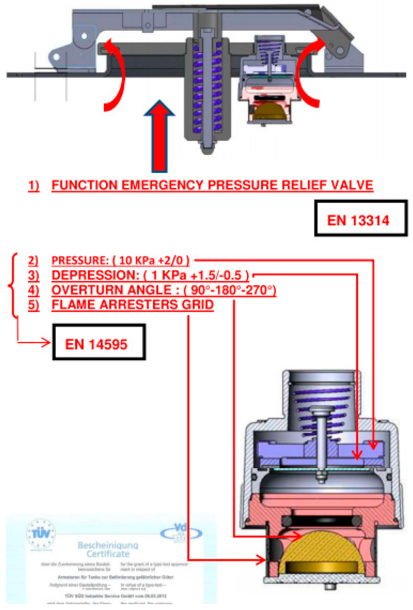
Article

Impact of Sloshing on Fossil Fuel Loss during Transport

by
Hafsa Mir
1,
Tahir Abdul Hussain Ratlamwala
2,
Ghulam Hussain
3,
Mohammed Alkahtani
4,5,* and
Mustufa Haider Abidi
5
1
Department of Mechatronics Engineering, SZABIST, Karachi 75600, Pakistan
2
Department of Engineering Sciences, National University of Sciences and Technology, Islamabad 44000, Pakistan
3
Faculty of Mechanical Engineering, GIK Institute of Engineering Sciences & Technology, Topi 23640, Pakistan
4
Industrial Engineering Department, College of Engineering, King Saud University, Riyadh 11421, Saudi Arabia
5
Advanced Manufacturing Institute, King Saud University, Riyadh 11421, Saudi Arabia
*
Author to whom correspondence should be addressed.
Energies 2020, 13(10), 2625; https://doi.org/10.3390/en13102625
Submission received: 26 April 2020 / Revised: 13 May 2020 / Accepted: 16 May 2020 / Published: 21 May 2020
(This article belongs to the Section E: Electric Vehicles)

Abstract

:
This study attempts to uncover the most common issue of fuel shortage faced by the oil and transportation industry worldwide. In Pakistan, petroleum is transported to the northern areas from the south coast. Currently, this is done using road tankers as a pipeline is still under construction. However, even after the pipeline becomes operative, road tankers would still be used for intra-city transport. Findings from this study can be used to determine the inter-city transport losses faced by oil companies. This study determines the hydrocarbons lost to the environment during inter-city road transport of petroleum. It takes nearly 2–3 days to complete a one-way trip with the fully loaded tank. Much work has been reported worldwide on hydrocarbon emissions, but nearly all of it has been done either for storage tanks/vessels or fuel tanks in rails/cars. The aim of this study was to investigate the actual amount of fuel lost to the environment due to the sloshing of liquid. Also, the results were expected to help in determining the extent of hazardous emissions resulting from road transport of petroleum. Hence, measures could be taken by the concerned authorities to mitigate the emissions if they exceeded the acceptable range. The sloshing was not found to contribute much in terms of vapor loss. Valve location was found to be important as no loss was obtained from the third compartment because the valve is to the right in this chamber. A negligible amount of fuel was lost from the first and second compartments per application of the brakes. Over a whole trip of 2–3 days, if the tanker braked 500 times, a total of 9–10 L would be lost to the environment.

1. Introduction

This study explicitly calculated the amount of fuel lost from a 48,000 L tank on a one-way trip from Karachi to Sheikhupura (Machike). The tank was comprised of three individual compartments of 16,000 L. Each compartment was fitted with a pressure/vacuum breather vent valve at the top of the tank to prevent the tank from creating overpressure/vacuum.
Besides the evaporation losses, the movement of the liquid inside the tank when it is subjected to harsh acceleration or brakes can also contribute to fuel loss. This is because the pressure exerted by the liquid on the tank walls can be substantial enough to reach the opening pressures of the P/V vent valve of the tank. The movement of the fluid after an impact produces large shifts of weight which build momentum and do not settle down easily. This movement of the liquid is termed ‘sloshing’.
A significant amount of work has been done on sloshing in tanks; particularly fuel tanks. Different kinds of road tanks have been taken into account. But nearly all of them investigate the impact of sloshing on the dynamics and stability of the vehicle. None of them have used the sloshing loads to determine vapor loss.
D’ Alessandro [1], mentions in his Ph.D. thesis that a lot of research has been done on sloshing because a statistical survey of the US Department of Transportation (US DOT) reported that each year 1300 tank truck rollovers occur, 56% of which occur on the straight road, 50% involve leaving the road, 98% occur on a dry road and only in 28% of the time was the driver driving too fast. Moreover, 31% of the fatalities in rollovers of commercial vehicles occur among tank trucks.
This study further investigates the effect of sloshing loads on the dynamic stability of the vehicle. To do so, the static rollover threshold is determined using the tilt table test. The least acceleration for wheel lift occurs at 70% volume fill i.e., the minimum static rollover threshold occurs at 70% fill. This highlights the effect of sloshing on the dynamic stability of the vehicle i.e., the minimum static rollover threshold occurs when the tank is not completely filled.
A lane-change maneuver is then studied to compare the lateral accelerations and roll angles of fluid and rigid cargo under the same testing conditions. The maneuver consists of lateral displacement of 3.5 m at a constant speed of 50 km/h and a steer-angle frequency of 0.5 Hz with a 50% fill volume. The difference between the results of fluid and rigid cargo is due to the sloshing loads in fluid cargo [1].
Seeing the effects of fluid slosh, many studies investigated methods of reducing slosh. Some have used computational fluid dynamics to come up with different solutions. Many have used the Finite Volume (FV) technique to solve the Navier Stokes equations using ANSYS. However, a disadvantage of FV is that mesh/grid calculation is a necessity. Some mesh-free methods like Smoothed Particle Hydrodynamics (SPH) or the Finite Pointset Method (FPM) have been widely used. Shadloo et al. [2] compared SPH with several methods requiring mesh. The authors concluded that SPH is an ideal choice for complex free-surface flows with very high deformations and moving geometry. However, they recommended using mesh-based methods in turbulence, slow flows without complex interfaces [2]. Lokman et al. [3] modeled the airflow inside a rotating machine using two CFD methods: FV and SPH. Since the SPH method does not require meshing, they save a lot of time. However, the authors pointed out that the FV method is quite robust yet expensive. The 3D SPH solver was found to represent well the overall flow pattern, but it failed to model the Taylor vortex flow inside the air-gap. Whereas, the FV method captured the Taylor vortex flow. The authors certainly felt that 3D SPH was not able to capture the Taylor vortex flow because of the limited number of particles used. The authors concluded that the SPH method could be used to model the flow inside rotating machines within a satisfactory accuracy [3]. Besides the mesh-free algorithms, the Lattice Boltzmann method (LBM) has also been used. Goodarzi et al. [4] compared FV and LBM for solving a natural convection problem. The natural convection on a laterally heated square enclosure filled with air was studied. The problem was solved using both the LBM and FV algorithm. The results were also compared with the experimental values and it was found that FV yields more accurate results compared to LBM. Also, FV was more time-efficient than LBM [4]. Sadeghi et al. [5] used LBM to study the phase transport in complex porous media. LBM was used to study the pore-scale level and the model was validated with analytical results. Hence LBM was recommended to be used in complex geometries such as porous media [5].
Besides, optimum baffle sizes and configurations to minimize sloshing loads on tank walls have been widely studied. Kuzniatsova and Shimanovsky analyzed baffle with and without perforations. A circular tank with a diameter of 2 m and a length of 4 m was taken into account. The fill-level was taken to be 60%. ANSYS CFX was used to simulate the scenario of emergency braking. A baffle with holes of 20 cm diameter was found to reduce the hydrodynamic pressures 4.5 times in comparison to the solid baffle [6].
Brar and Singh [7] analyzed an elliptical tank with various configurations of baffles. CFD simulation was used. The numerical analysis was validated using experiments and no significant variations were found. An elliptical tank carrying 15,000 L petrol was taken into account. A frequency of 1 Hz was used and sudden retardation was applied. The truck stopped after 6 s.
Three cases were considered:
  • No baffles
  • Three vertical baffles
  • One horizontal and two vertical baffles
Out of these, the most reliable i.e., the one with least slosh was with three vertical baffles [7].
Joshi et al., compared the average and maximum impact pressures of different fill levels using CFD. This was done for a chamfered LNG road tank. The dimensions of the chamfered tank were 1.3 m × 0.9 m with a 45 degree chamfer, 30 cm offset chamfer. The simulation was performed with and without baffles for each fill-level. Five different monitor points were selected each on the vertices of the tank to find the maximum impact locations. Fill levels of 30, 50, and 80 were used. Baffles seemed to mitigate the impact pressures at all points and fill levels. However, for low filling levels, baffles seemed to mitigate the impact pressures nearly by a factor of 10 [8].
Močilan et al. performed a CFD analysis on a fuel tank using ANSYS FLUENT. The proportion of fuel to air was 60:40 and time-varying acceleration was applied. The free surface was modeled. Also, the maximum stress in the tank was found. The research found that reduced amounts of stress levels were found with baffles as opposed to a tank without baffles [9].
In another study, Siddapureddy and Satapathy performed CFD on a rectangular tank with dimensions 5 × 4 × 4 m3. The software used was FLUENT. The tank was partially filled with water. The tank started from rest. In the first two seconds, it rose to 30 km/h and remained at 30 km/h for another 4 s. Then in the last two seconds, the velocity decreased from 30 km/h to 0 km/h. In the study, three different fill levels of 30%, 50%, and 70% were analyzed. The exercise of different fill levels was repeated for tanks without baffles, with horizontal baffles, with vertical baffles, and with multiple baffles. Also, the simulation results were validated by experiments. It also introduced a new concept of percentage reduction (PR) which was calculated using mean deviation (MD). MD is the mean of the deviations from the mean position i.e., the position of the free surface at the start of the simulation. Hence, PR can be used to assess the performance of different baffle designs. Results found that vertical baffles were more efficient in contrast to horizontal ones. However, multiple baffles showed better results than horizontal/vertical ones where minimization of the sloshing effect was more crucial than the complexity of the design of the tank [10].

2. Methodology

2.1. Valve Model

The tank is fitted with a Breather Vent Valve in each compartment to prevent overpressure/vacuum [11,12]. The tank is composed of three compartments each of 16,000 L capacity. Hence, three P/V Vent valves are present in total. The threshold absolute pressures of the valve are in compliance with EN 14595 [13,14] as shown in Figure 1:
  • In pressure: 111 kPa (+2/−0)
  • In vacuum: 100 kPa (+0.5/−1.5)
The valve is also fitted with a spill over protection which prevents the spillage of fuel when a rollover occurs.
The flow rate of the valve was modeled. The cracking pressure of the valve is 111,000 Pa. Hence, the model was divided into three regions:
  • Valve closed: This is when the pressure is below 111,000 Pa.
Q = 0
2.
Valve partially open: This is when pressure is between 111,000 and 131,323 Pa. Two data points were provided by the manufacturer [15] which are shown in Table 1 below:
These data points were used to form the equation of this region:
Q = 6.18025 × 10 47 e 0.0009 P
3.
Valve fully open: This is when the pressure is equal to or greater than 131,323 Pa. Hence,
Q = 132,000 L/h
The flow rates of each region are summarized in Table 2.
The below graph (Figure 2) shows the behavior of the valve in all three regions. A curve fit was done to determine the equation of region 2, however, flow rates of region 1 and region 3 were directly supplied by the manufacturer.

2.2. Computational Fluid Dynamics

Sloshing is the movement of the free surface when the tank is subjected to acceleration/deceleration. The CFD method solves Navier Stokes equations of momentum and heat and mass transfer. This was performed in ANSYS CFX. CFX uses the finite volume technique to solve these equations. In this technique, the area of interest is divided into smaller regions called control volumes. The equations are solved numerically for each control volume [16].
A multiphase sloshing simulation was set up to determine the hydrodynamic pressures generated. These pressures were then used to estimate vapor loss.

2.2.1. Sensitivity Analysis

A sensitivity analysis was performed on the elliptical tank to determine the spatial and temporal coordinates where the desired convergence was achieved. A general Gaussian waveform of acceleration with a peak of 2.6 m/s2 i.e., 0.265 g was applied as shown in Figure 3. An initial velocity of 0.2 m/s was applied. The period of the wave was kept at 5 s. Peak acceleration of 2.6 m/s2 was applied because it was obtained from the tracker report of the truck. The simulation was run for 1 s in each case.
The mesh was generated using a curvature size function. The curvature size function was used because of the curvature in the geometry. The function examines curvature on edges and faces and forms elements without exceeding the maximum element size and the curvature normal angle specified. The CFX solver calculates the curvature normal angle, growth rate, and minimum edge length based on the geometry. The remaining parameters (minimum face size, maximum face size, and maximum size) were decided from the results of the sensitivity analysis. Initially, the following values were used as shown in Table 3:
A length of 0.04 m was selected as the mesh size and 0.1 s as the time step size. The detailed results from the sensitivity analysis are shown in the results section.

2.2.2. Basic Set-Up

A multiphase simulation was setup in ANSYS CFX. For simplicity, one compartment of the tank was simulated. The geometry was imported from Solid Works. The multiphase homogeneous flow was modeled and gravitational acceleration was applied. A mesh sensitivity analysis was performed to determine the coordinates where convergence was achieved. These coordinates were then used in further simulations to analyze different scenarios. The velocities and accelerations against each time step for each case were recorded in an excel file. The excel file was then given as input to ANSYS CFX. Properties of air and octane [17] were used as shown in Table 4 and Table 5.
Air:
Table 4. Properties of air.
Density1.185 kg/m3
Molecular Weight28.96 (kg/kmol)
Dynamic Viscosity 1.831 × 10 5 (Pa s)
Thermal Expansivity0.003356 (K−1)
Specific Heat Capacity1004.4 (J/kg K)
Thermal Conductivity 2.61 × 10 2   (W/mK)
Octane:
Table 5. Properties of octane.
Density740 (kg/m3)
Molecular Weight114.2 (kg/kmol)
Dynamic Viscosity0.00051 (Pa s)
Thermal Expansivity0.00095 (K−1)
Specific Heat Capacity2240 (J/kg K)
Thermal Conductivity0.15 (W/mK)

2.2.3. Monitor Points

Pressures are measured at points beneath the vent valve. The location of the valve is slightly different for each compartment. Hence, pressures are monitored at all three locations of the vent valve. However, this is done on a single compartment. The following figure is of a 48,000 L tank with three chambers (Figure 4). The tank is comprised of three chambers each of 16,000 L capacity.
Three monitor points were selected (Figure 5):
  • This point was selected to be directly below the valve of the third compartment. The cartesian coordinates are [0, 1.92, −2.49].
  • This point was selected to be directly below the valve of the first compartment. The cartesian coordinates are [0, 1.92, −1.72].
  • This point was selected to be directly below the valve of the second compartment. The cartesian coordinates are [0, 1.92, −1.78].

2.2.4. Acceleration/Deceleration Function

Different cases were analyzed using various acceleration/deceleration functions. The acceleration/deceleration behavior of trucks and a truck-trailer combination was studied. This was done to develop realistic acceleration/deceleration functions to come up with accurate vapor loss generated through sloshing.
The Verizon Telematics [19] describes the minimum and maximum thresholds for hard braking and hard acceleration for light- and heavy-duty vehicles. For light-duty vehicles, it gives a minimum and maximum acceleration threshold of 0.36 g and 0.8 g respectively. For heavy-duty vehicles, it gives a minimum and maximum braking threshold of 0.22 g and 1 g respectively.
The Highway Safety Research Institute described the braking performance of trucks and tractor-trailer combinations by performing several tests [20]. It describes a test named ‘brake effectiveness test’. In one such test, the tractor-trailer was moving at 30 mph and the brakes were applied until the vehicle stopped. The deceleration was found to be −0.38 g and the stopping distance was 100 feet. The values from this test were used to form the normal acceleration/deceleration function because the deceleration and the cruising speed of our tractor-trailer are in close comparison to the parameters in this test.
The maximum values of deceleration from a test just before jack-knifing occurred were used to develop the abnormal case of deceleration/acceleration. The initial velocity was 30 mph and the maximum deceleration was −0.55 g with a stopping distance of 77 feet. The values from this test were used to form the abnormal acceleration/deceleration function because no wheel lock occurred at this value. The input functions were derived considering all the above information. Four cases were analyzed:
  • Acceleration—normal case: The values (acceleration, distance covered) were kept similar to the values of one of the tests of the brake effectiveness test [20]. The vehicle started from 0.2 m/s and rose to 12.96 m/s in 4.7 s after covering a distance of 29.5 m. The maximum acceleration was 0.4 g. Velocity and acceleration curves are shown below (Figure 6 and Figure 7):
2.
Acceleration—abnormal case: The values (acceleration, distance covered) were kept similar to the maximum values of one of the tests of the brake effectiveness test [20]. The vehicle started with an initial velocity of 0.2 m/s and rose to 13.24 m/s in 3.9 s after covering a distance of 27.9 m. The maximum acceleration was kept at 0.55 g. The acceleration and velocity graphs are shown below (Figure 8 and Figure 9):
3.
Deceleration—normal case: The values (acceleration, distance covered) were kept similar to the values of one of the tests of the brake effectiveness test [18]. The vehicle started from 13.5 m/s and came to rest in 5 s after covering a distance of 31 m. The maximum acceleration was −0.4 g. The velocity and acceleration curves are shown below (Figure 10 and Figure 11):
4.
Deceleration—abnormal case: The values (acceleration, distance covered) were kept similar to the maximum values of one of the tests of the brake effectiveness test [20]. The vehicle started from 16 m/s and came to rest in 4.4 s after covering a distance of 27 m. The maximum acceleration was −0.51 g. The velocity and acceleration curves are shown below (Figure 12 and Figure 13):

3. Results and Discussion

3.1. Slosh Calculation Validation

3.1.1. Comparison of Numerical Results with Theoretical Values

A simple model of a rectangular tank was designed to cross-check the simulation results. The dimensions of the rectangular tank were 4.164 m × 2.48 m × 1.94 m (LXWXH). Fluid heights of 0.25 m, 0.5 m, 1.5 m, and 1.74 m were analyzed.
The lowest mode slosh frequencies were calculated using the following formula [21]:
ω n 2 = π ( 2 n 1 ) g a tanh π h ( 2 n 1 ) a
Next, the frequency and time period were calculated:
f = ω 2 π
t = 1 f
Here, a is the length of the tank, and h is the height of fluid in the tank. Hence, four different frequencies were calculated for each fluid height. Corresponding periods were calculated for each height.
The sloshing simulation was set up. Exactly the same rectangular tank was used as in the theoretical calculation. A gentle Gaussian acceleration pulse of 0.1 g was applied for 1 s as shown in Figure 14 and the simulation was run for 10 s. It was run for a long enough duration so as to determine adequate wave periods to establish confidence in the simulation results.
From sloshing simulation, periods of the following three parameters were compared with the theoretical calculation for each fluid height:
  • The pressure at a fixed monitor point at the top of the tank just beneath the valve
  • Maximum height of the free surface
  • Minimum height of the free surface
The periods of these three parameters were compared with the calculated period. In the case of pressures, the period was measured conventionally i.e., the difference between two consecutive peaks/troughs was taken because it was measured at a fixed point. However, in the case of heights, the period completes between three consecutive peaks/troughs as it was a half-wave i.e., mode 1 [22] as shown in Figure 15. This was because heights were not measured at a fixed point, rather, the software showed the maximum/minimum height of the free surface.
The numerical results were found to be in close comparison to the theoretical calculation in all three cases—pressure, maximum, and minimum height (Figure 16, Figure 17 and Figure 18). The simulation and calculation were performed for four different fluid heights of 0.25 m, 0.5 m, 1.5 m, and 1.75 m. In Figure 16, Figure 17 and Figure 18, the calculated periods at each fluid height almost overlie the periods obtained from the simulation. These results were used to build confidence in the slosh simulation setup. The same setup was then used on the cases to be analyzed. Screenshots from the simulation are shown in Appendix A.

3.1.2. Sensitivity Analysis

Before analyzing the actual cases in the actual tank, a sensitivity analysis was performed to gain confidence in the mesh size being used along with an acceptable time step. Screenshots from the simulation can be seen in Appendix A.
Spatial: The spatial coordinate was varied by changing the maximum element size in the curvature size function while keeping everything else constant. These were varied between 0.1 m and 0.03 m. The desired convergence was achieved at 0.04 m as shown in Table 6. The maximum pressure generated for mesh sizes of 0.04 m, 0.035 m, and 0.03 m was 1.0136 × 10 5 Pa. Hence, 0.04 m was selected as the mesh size.
The maximum generated pressures inside the tank were recorded for each mesh size for 1 s with a time step size of 0.1 s in each case. Pressures generated at 0.04 m, 0.035 m, and 0.03 m almost showed the same trend. Therefore, 0.04 m was selected as the mesh size. The results are shown in Figure 19 below:
Temporal: The time step was varied between 0.05 s and 0.25 s. The desired convergence was achieved at higher step sizes of 0.2 s and 0.25 s as well, but 0.1 s was selected so as not to lose too much detail. However, 0.05 s was not selected because of time constraints. The maximum generated pressures vs. time step size are summarized in Table 7.
The maximum pressure was recorded for each time step size for the duration of 1 s. The pressure values with a step size of 0.1 s almost follow the same trend as the values with a step size of 0.05 s. Hence, 0.1 s was selected as the step size due to time and resource constraints. The results are shown in Figure 20.

3.2. Slosh

Hydrodynamic pressures were recorded. In the case of deceleration, much higher pressures were produced because the fluid hits the valve with greater pressure compared to the acceleration scenario. Also, the valve opening pressures were reached only for the first and second compartments. This is because the valve is located towards the front of the tank in these compartments.
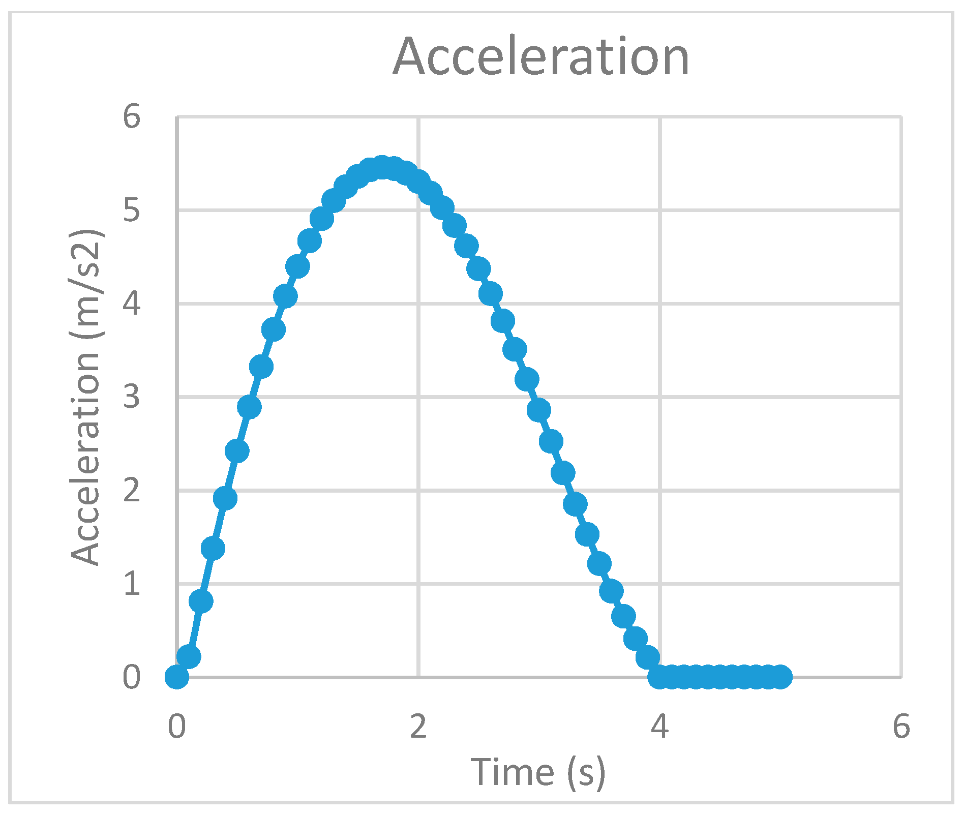
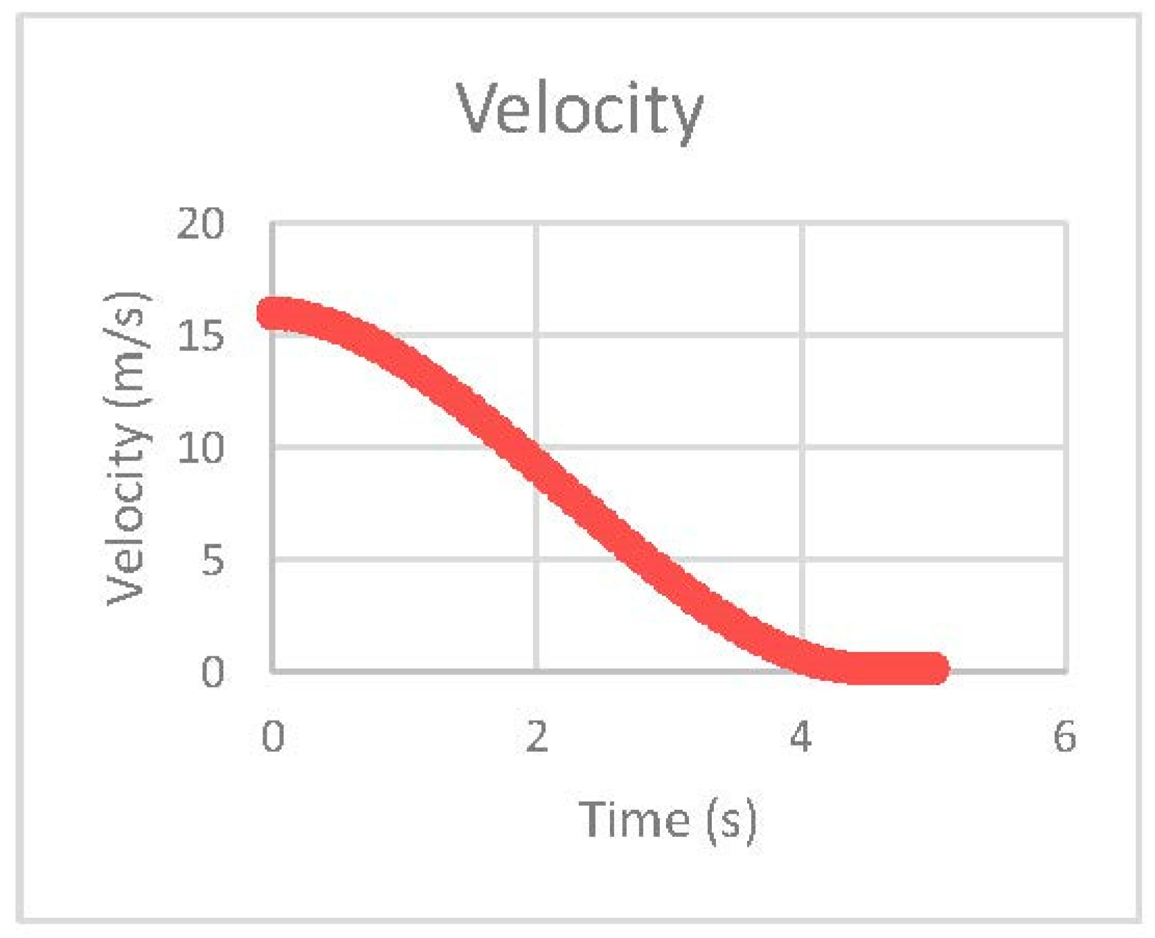
Case 1: Normal Acceleration
The slosh results i.e., the pressures generated with respect to time at all three monitor points for Case 1 are shown in Figure 21. The opening pressure of the valve i.e., 111 kPa was not reached at any monitor point. The least pressures were produced at Monitor Point 1 i.e., third compartment. The reason was its location i.e., it was placed farthest from the left and the tanker was moving towards the left. However, a similar trend of pressures was obtained for Monitor Points 2 and 3.
Case 2: Abnormal Acceleration
The slosh results i.e., the pressures generated with respect to time at all three monitor points for Case 2 are shown in Figure 22. In this case, as well, the opening pressure of the valve did not reach any monitor point. Similar to case 1, the least pressures were generated in the third compartment.
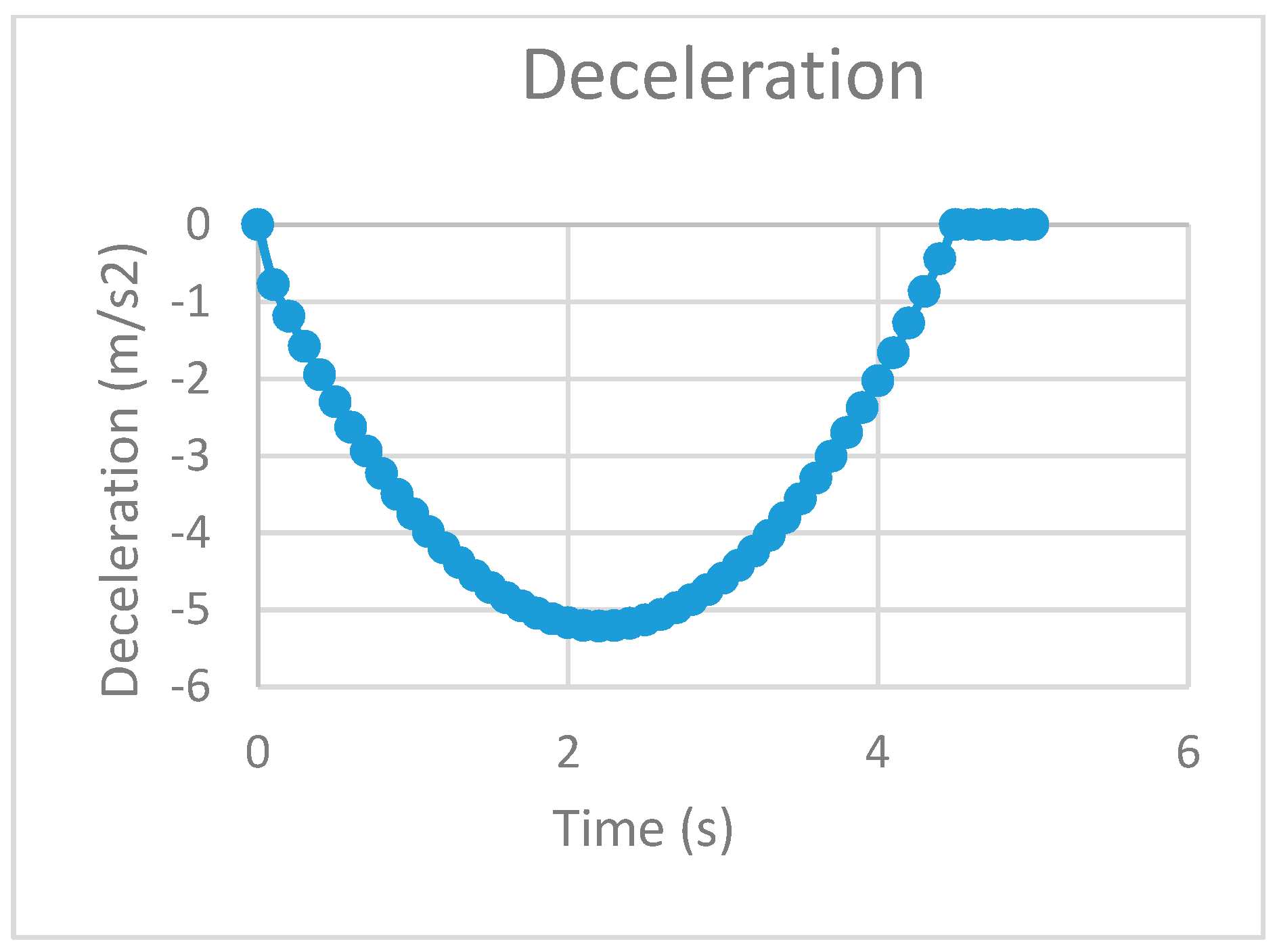
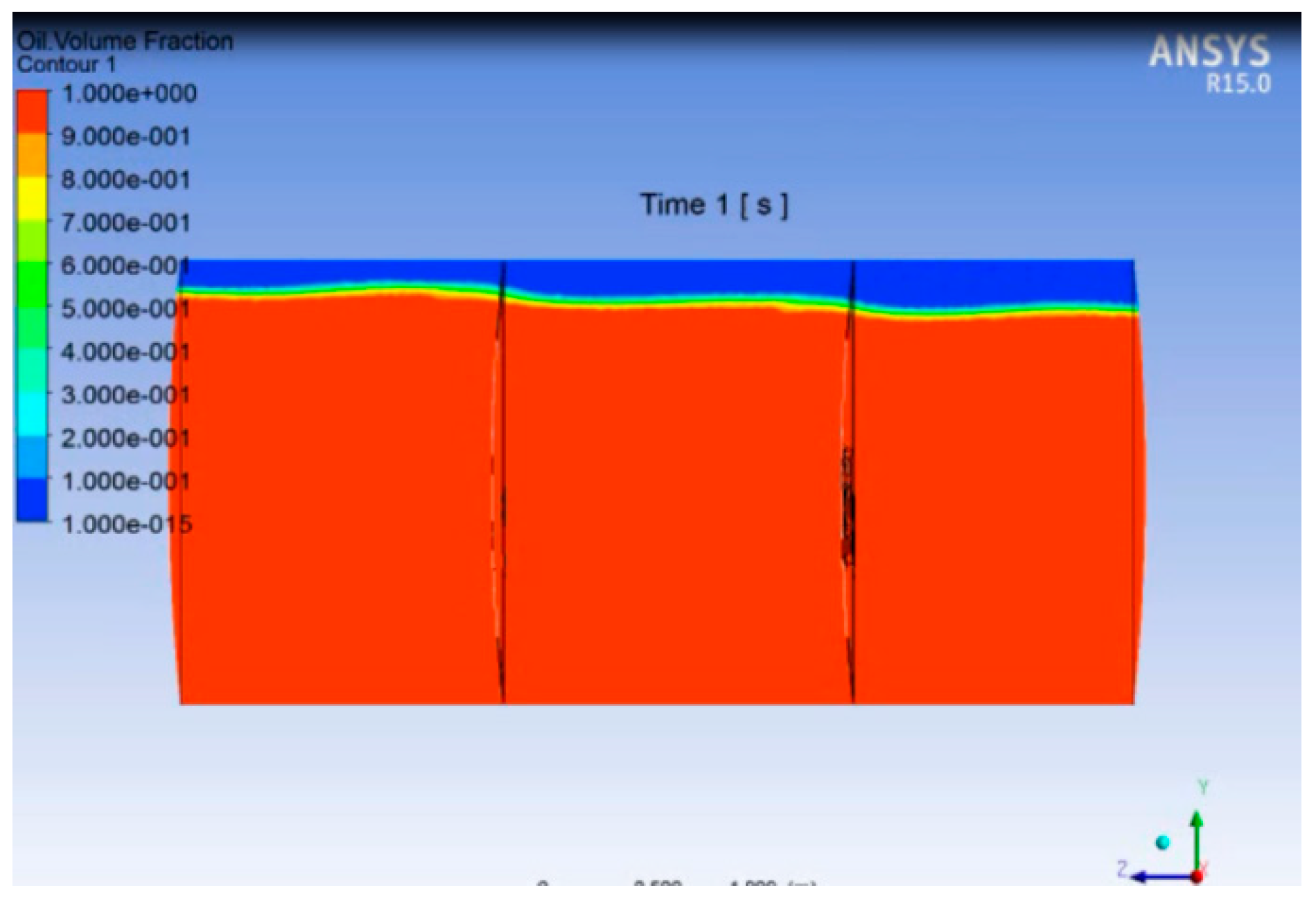
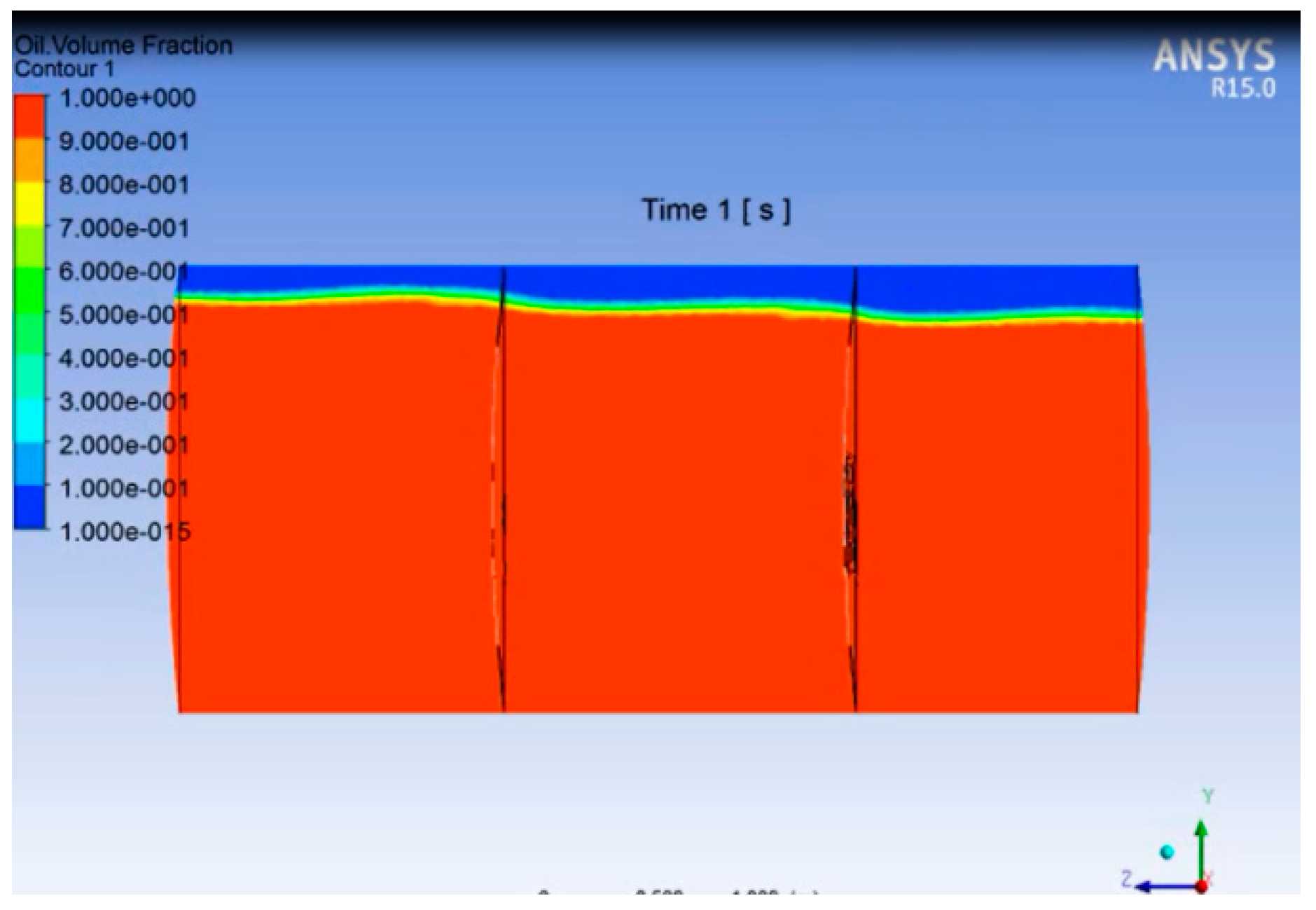
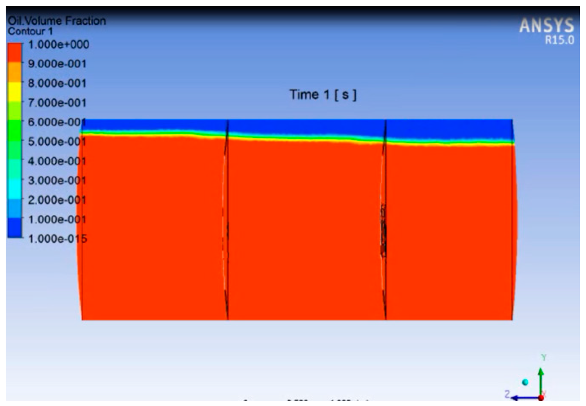
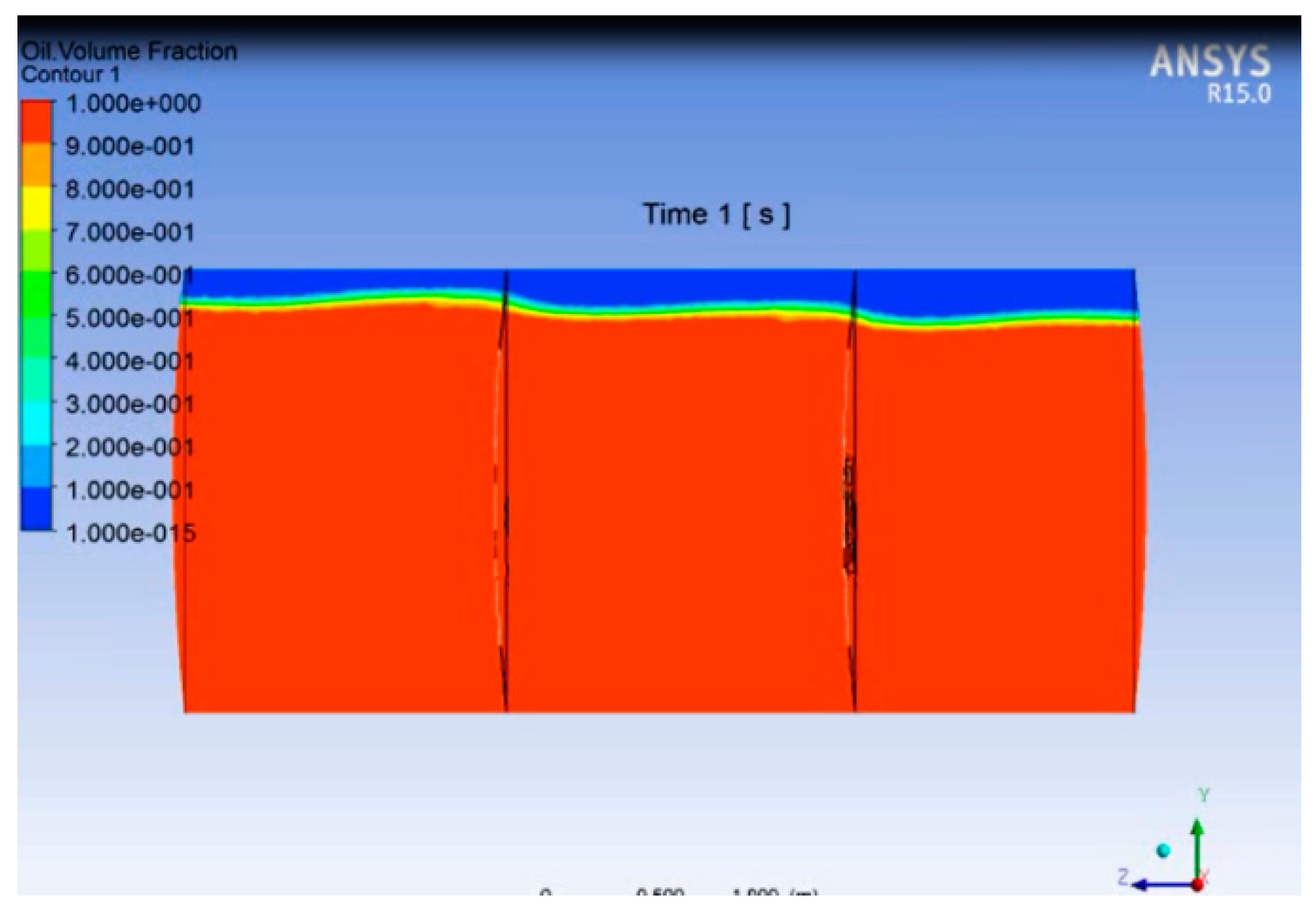
Case 3: Normal Deceleration
The slosh results i.e., the pressures generated with respect to time at all three monitor points for Case 3 are shown in 
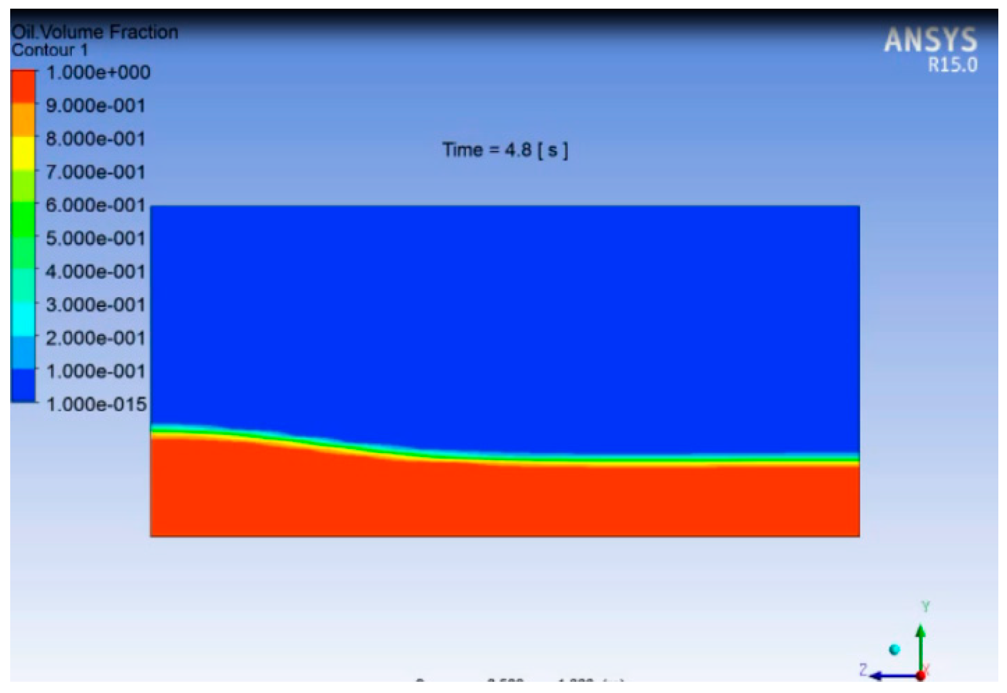
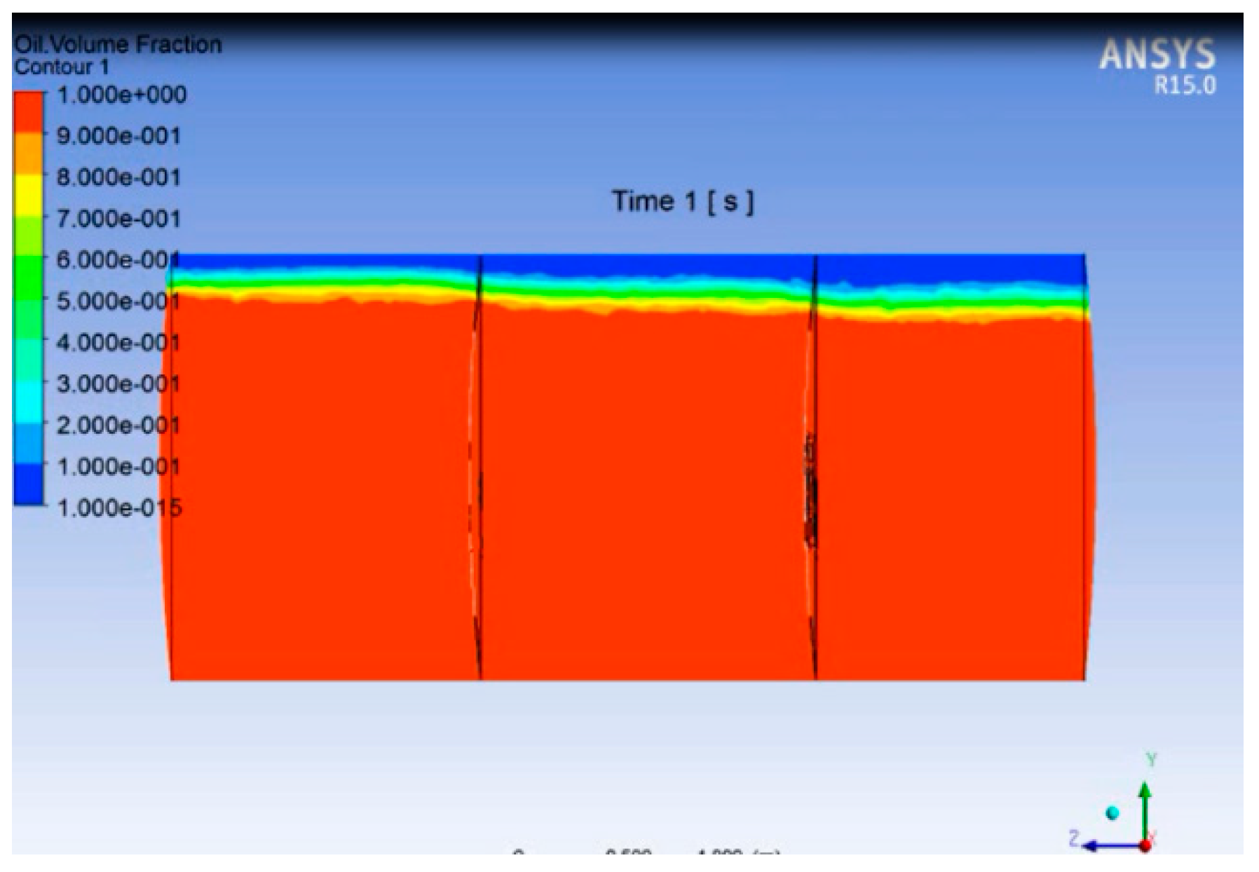
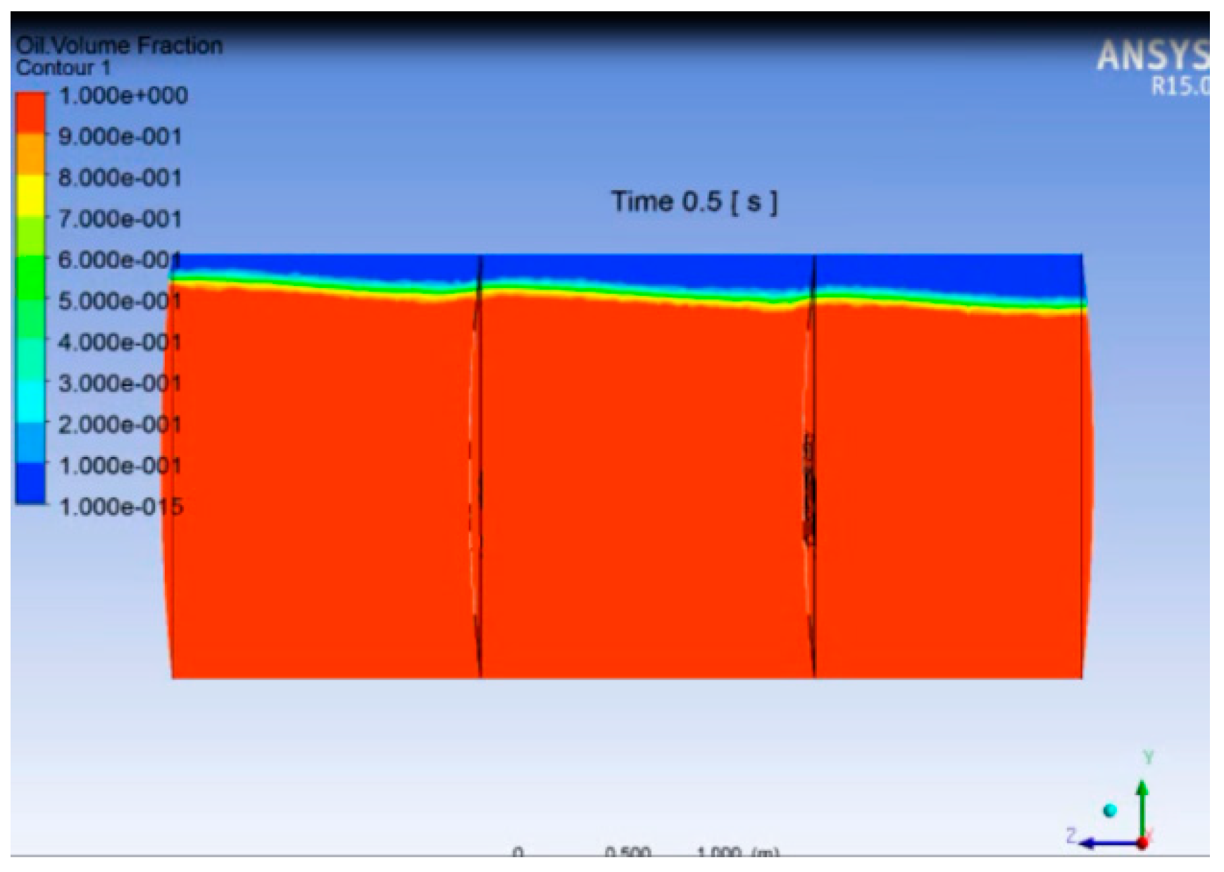
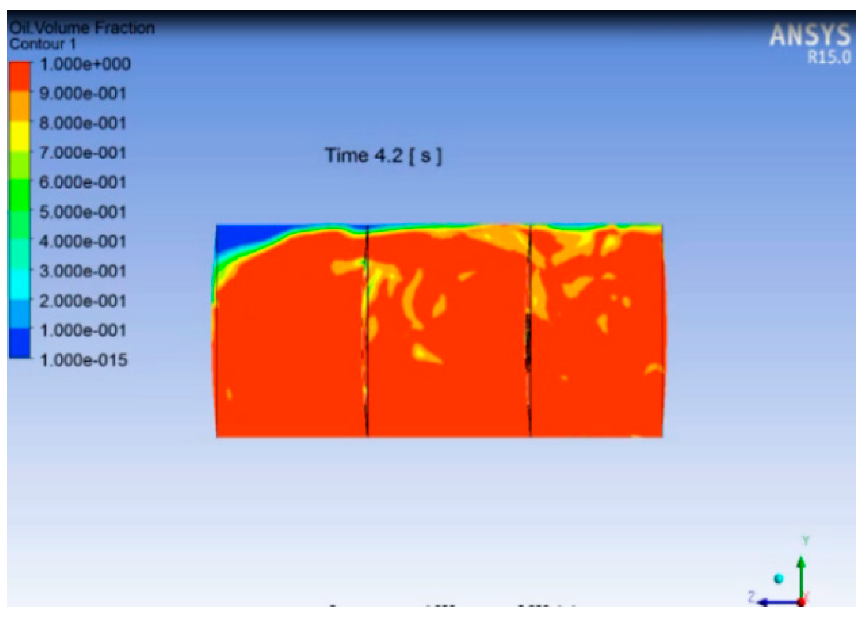
Figure 23. Opening pressures were exceeded for the first 0.2 s at point 2 and point 3. Also, an air pocket was found beneath the valve when the valve opens i.e., for the first 0.2 s (Appendix A, Figure A31). This confirms that the air/vapor mixture leaked out during that interval.
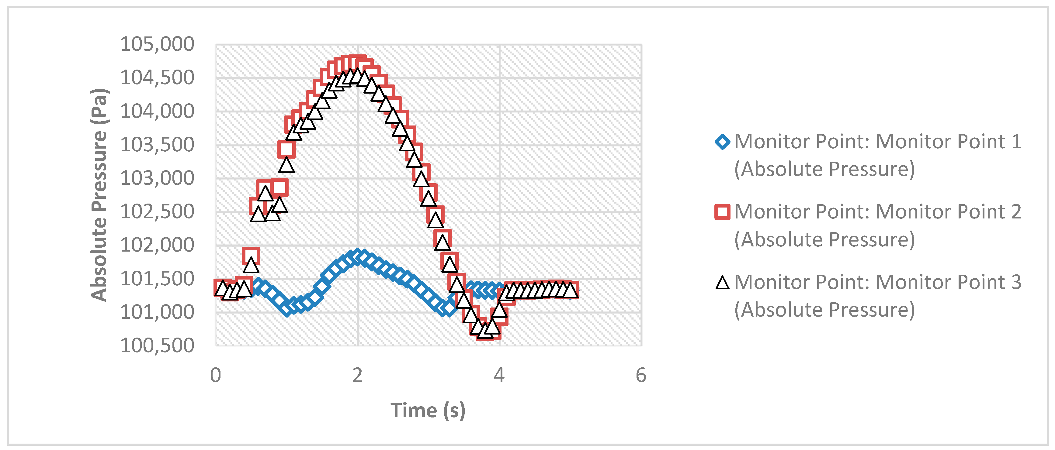
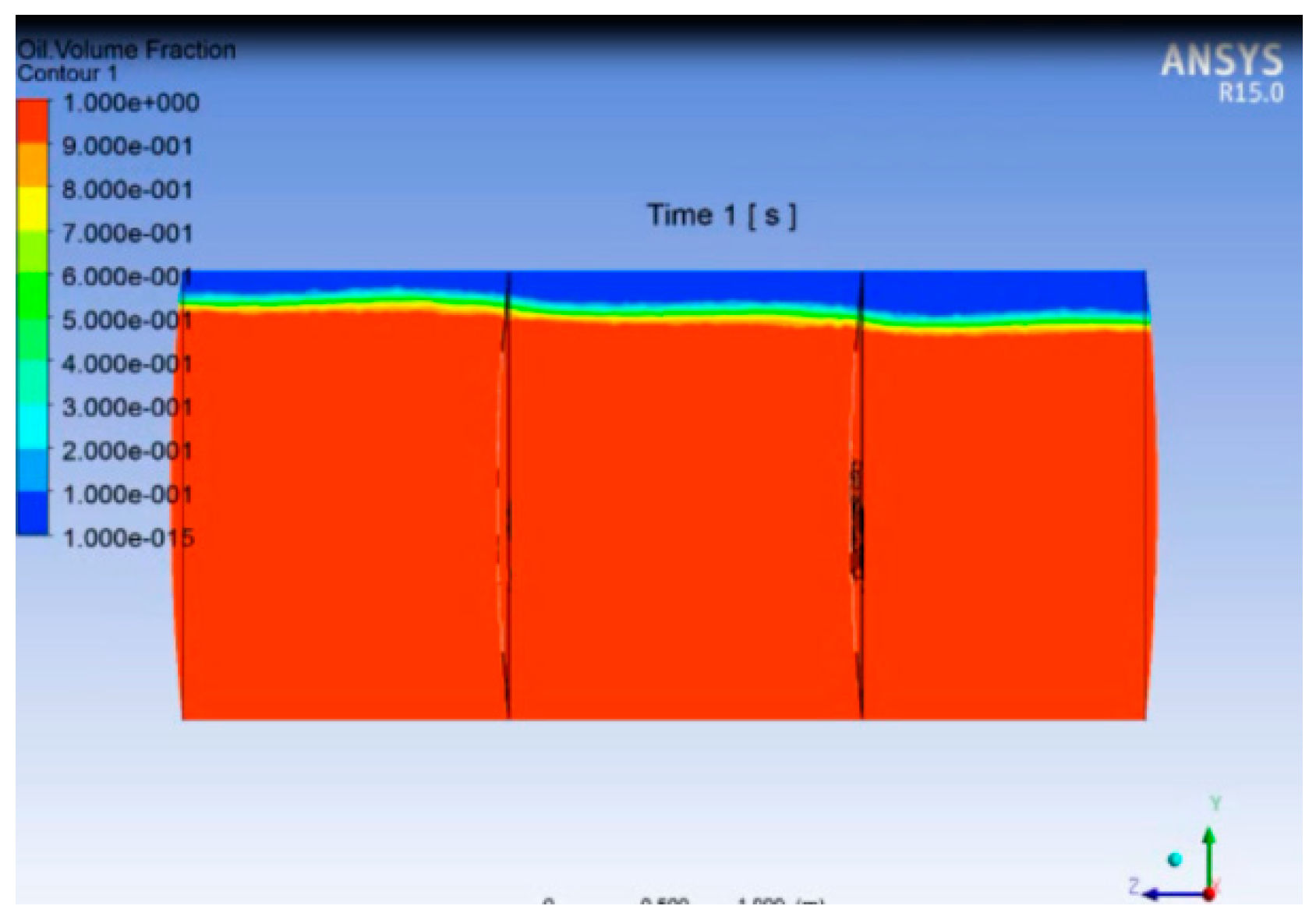
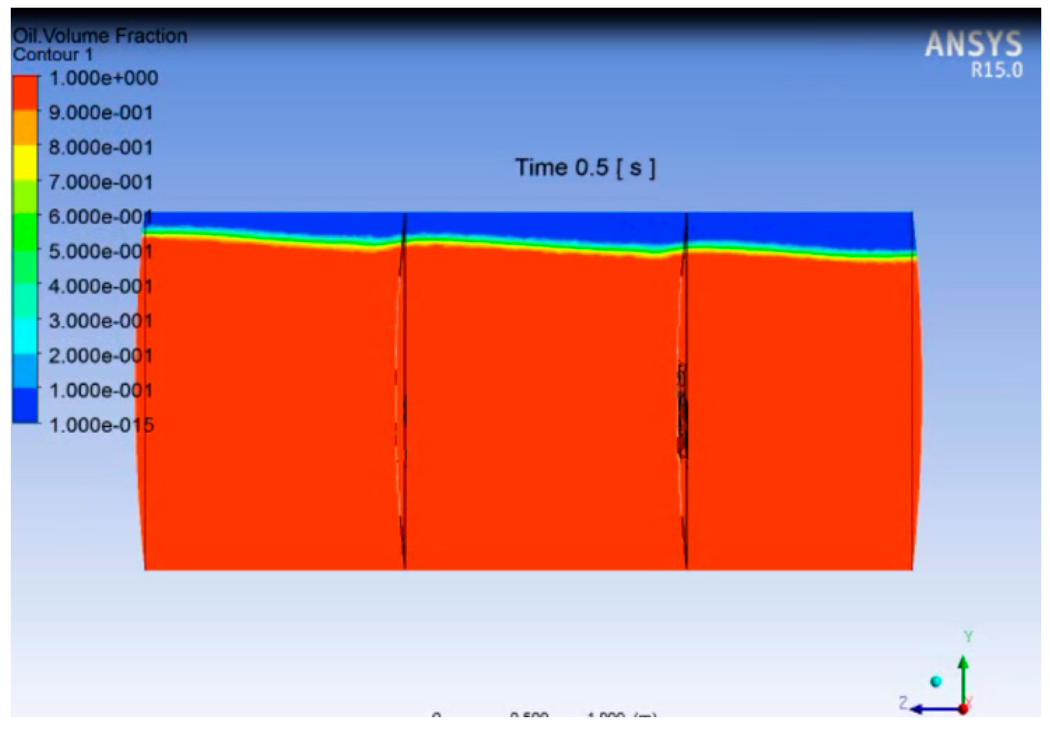
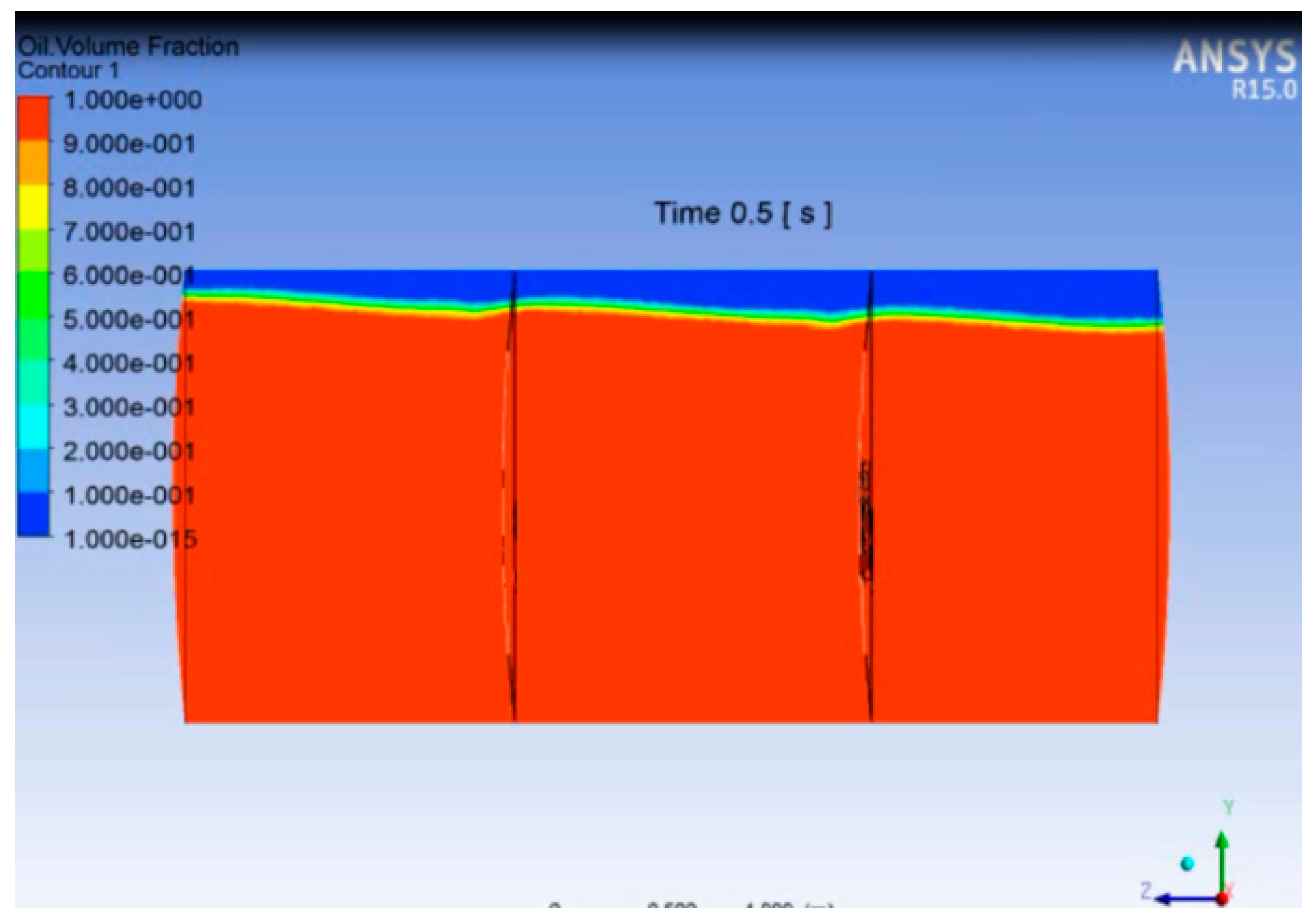
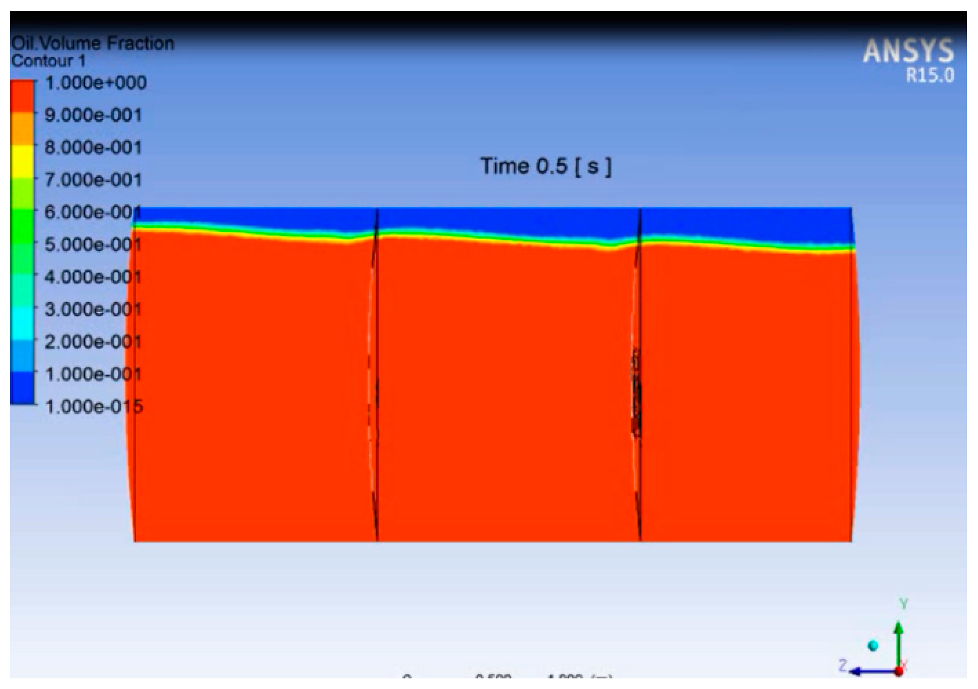
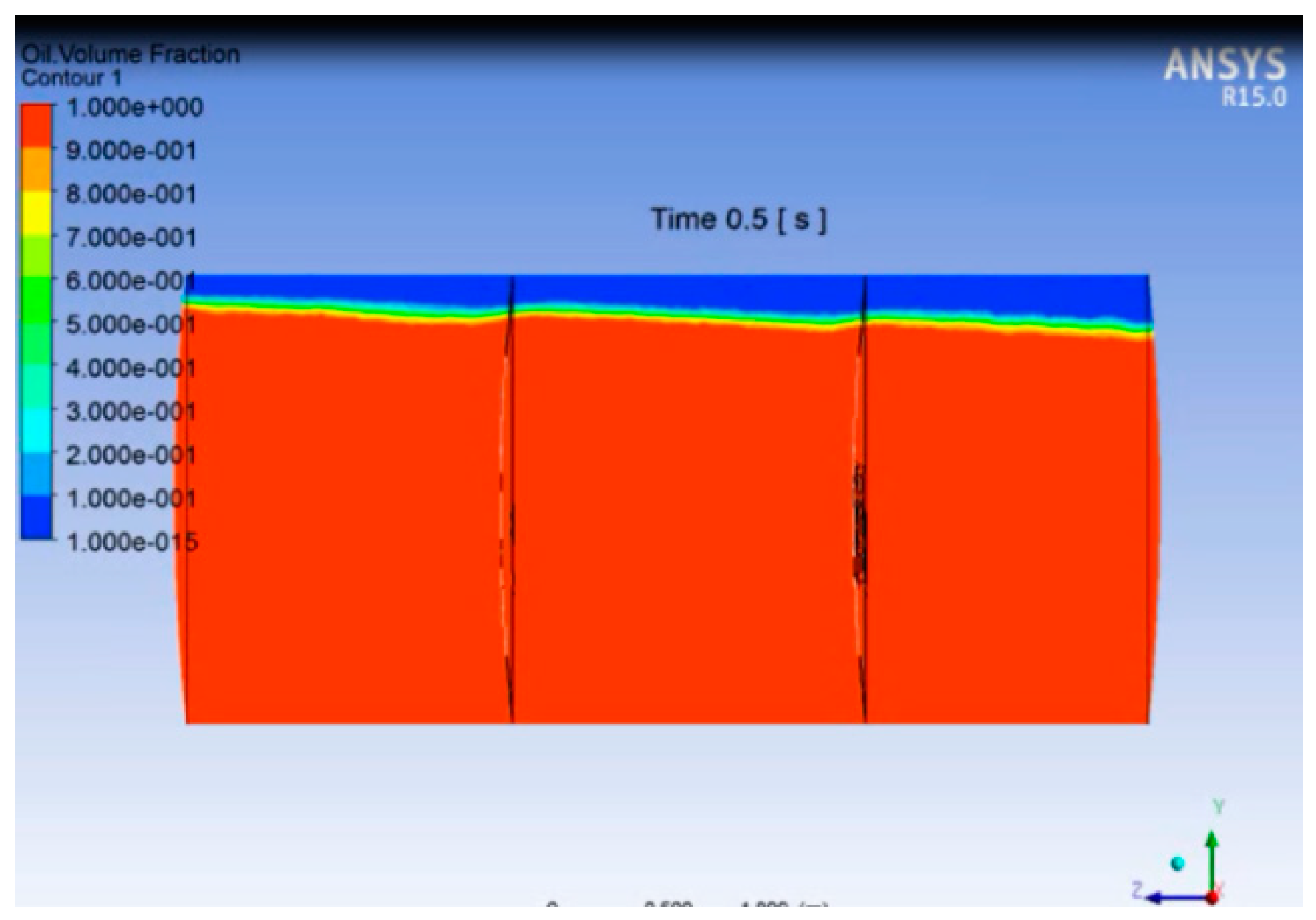
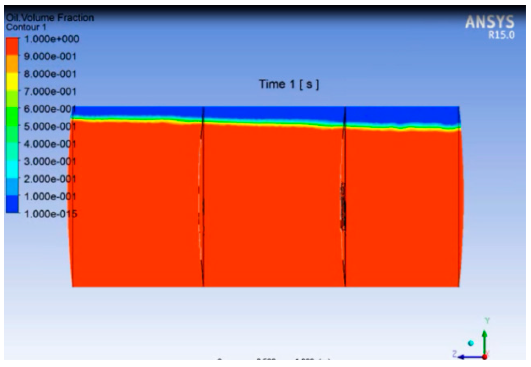
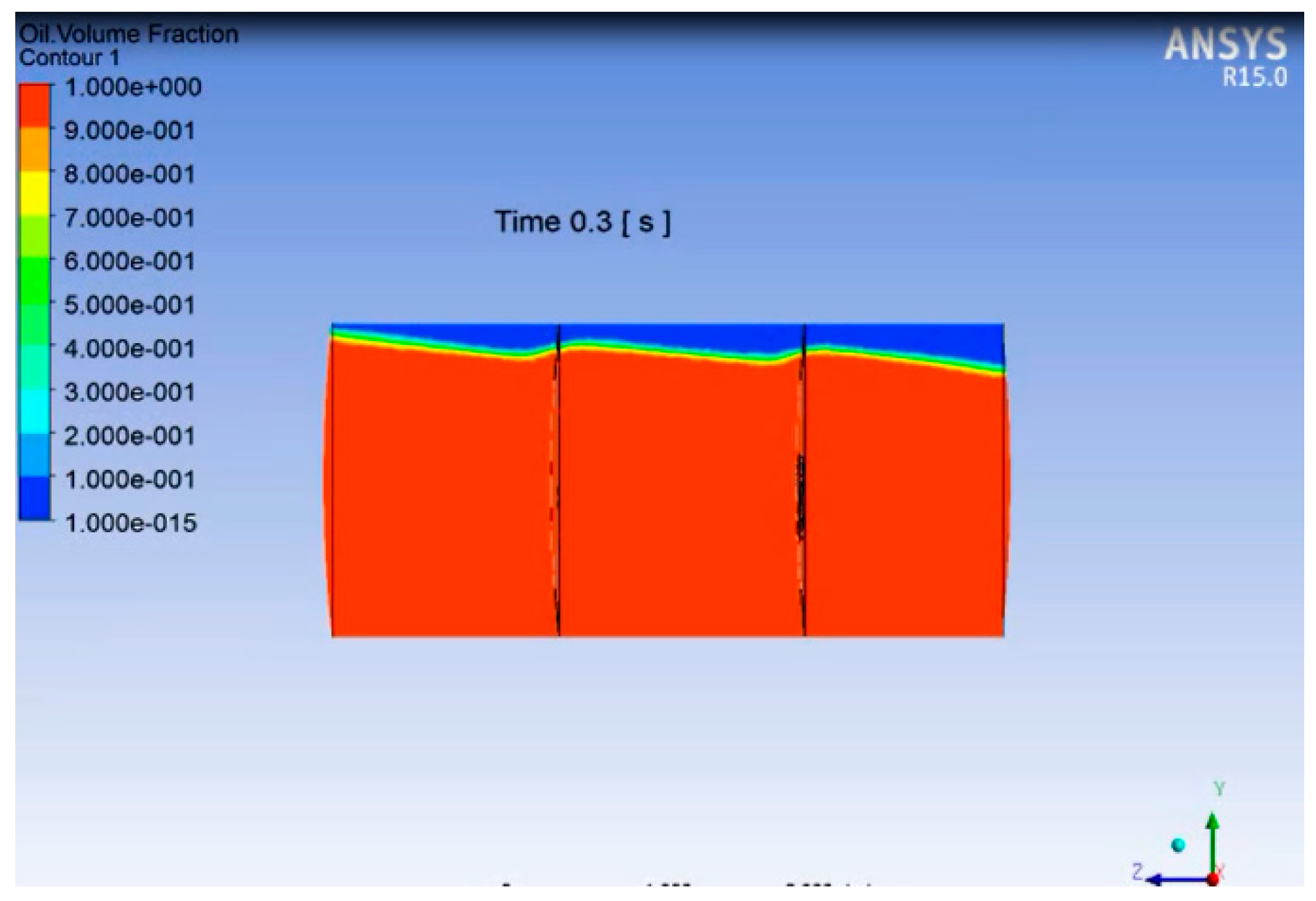
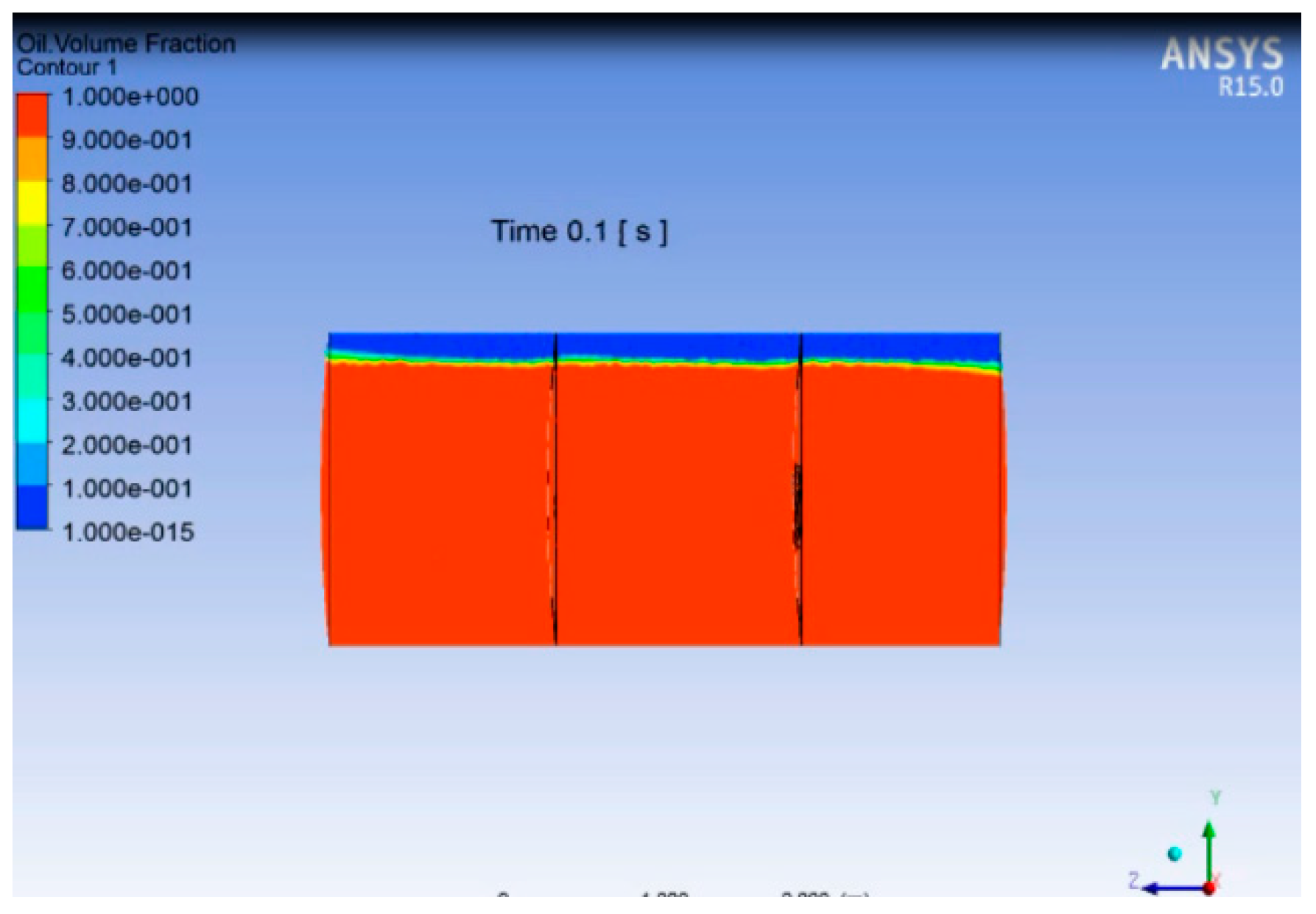
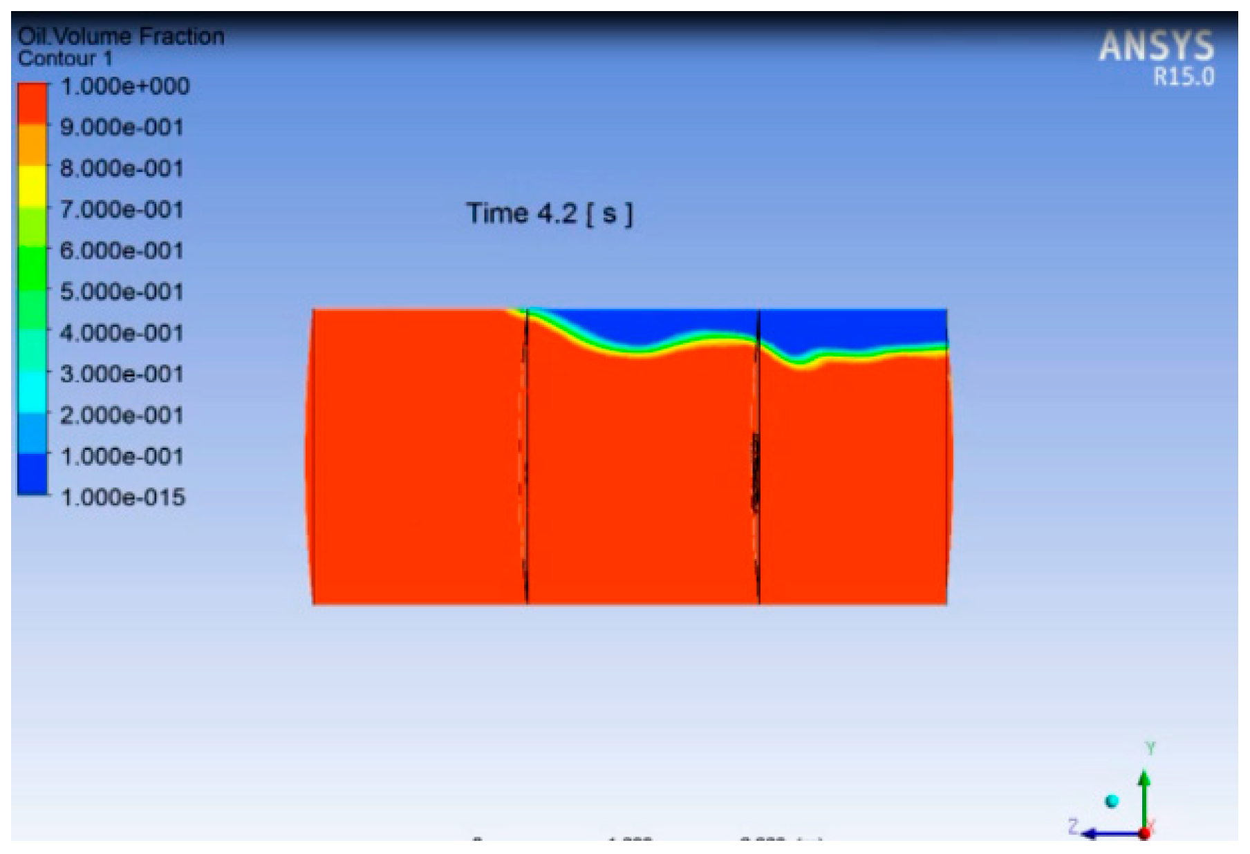
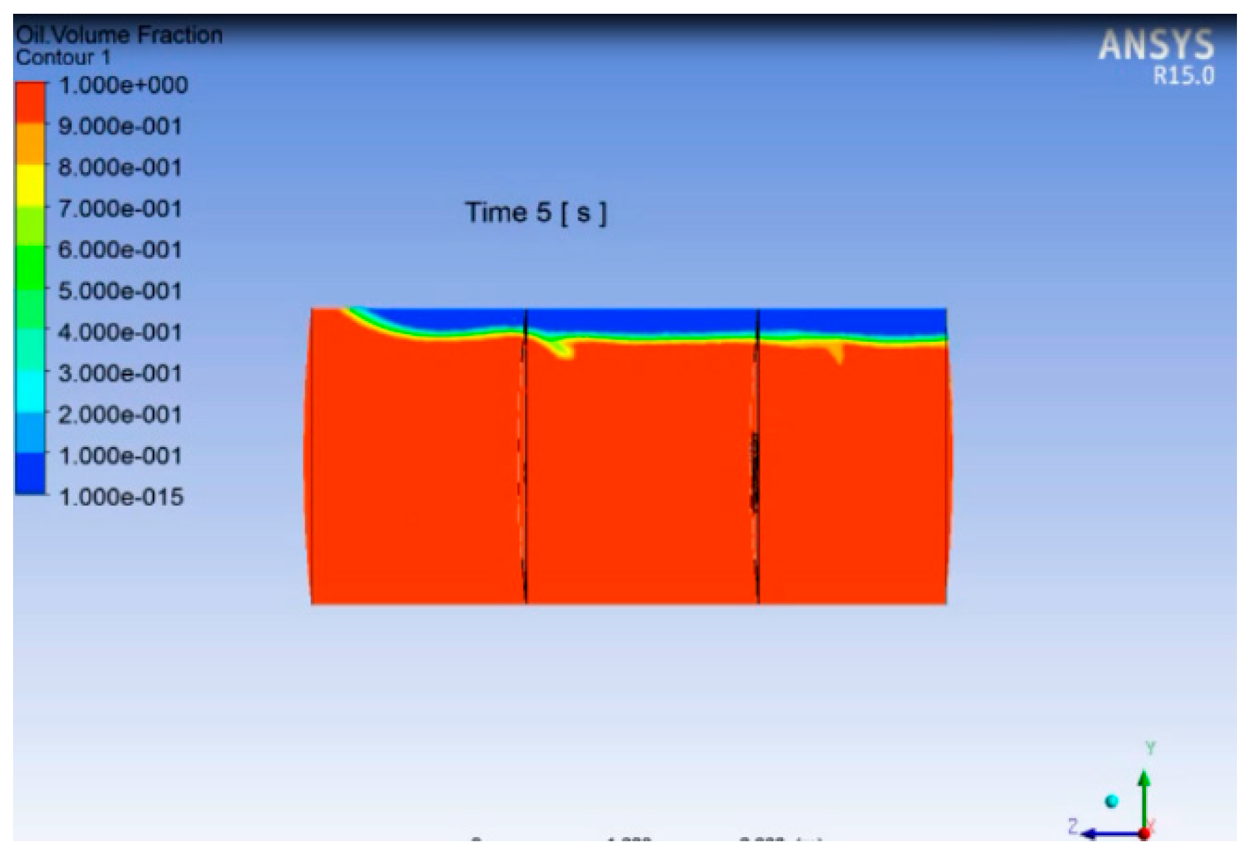
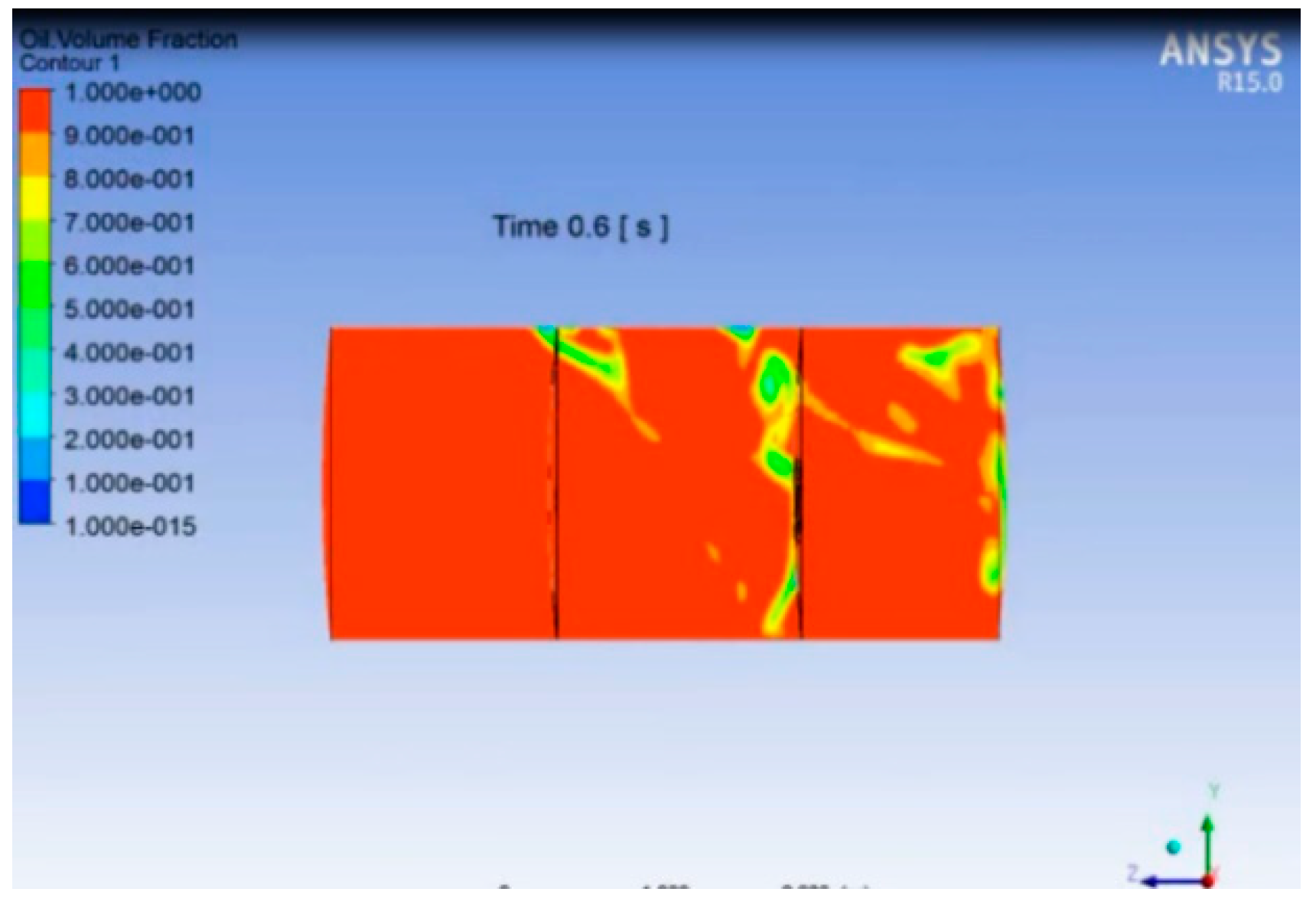
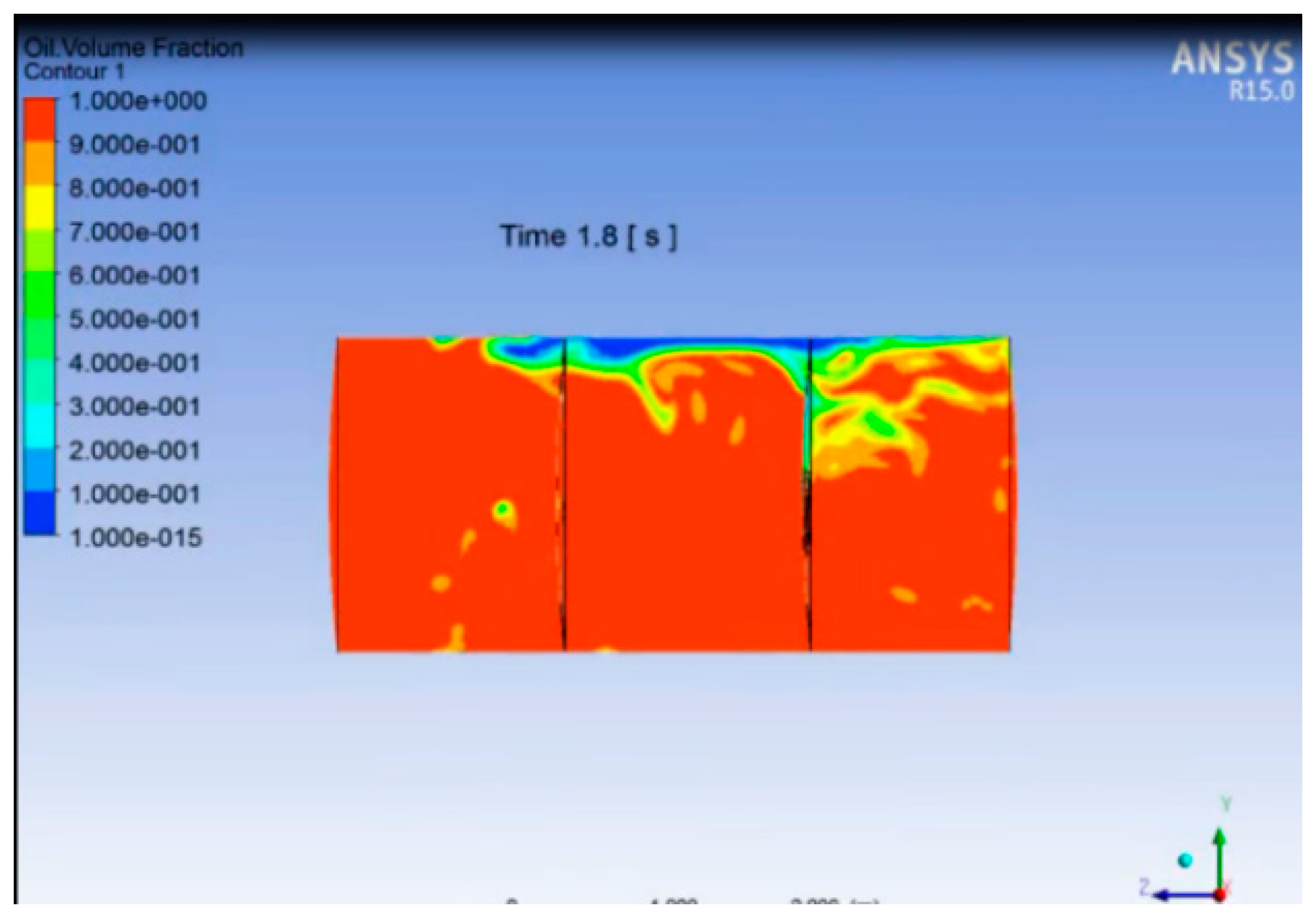
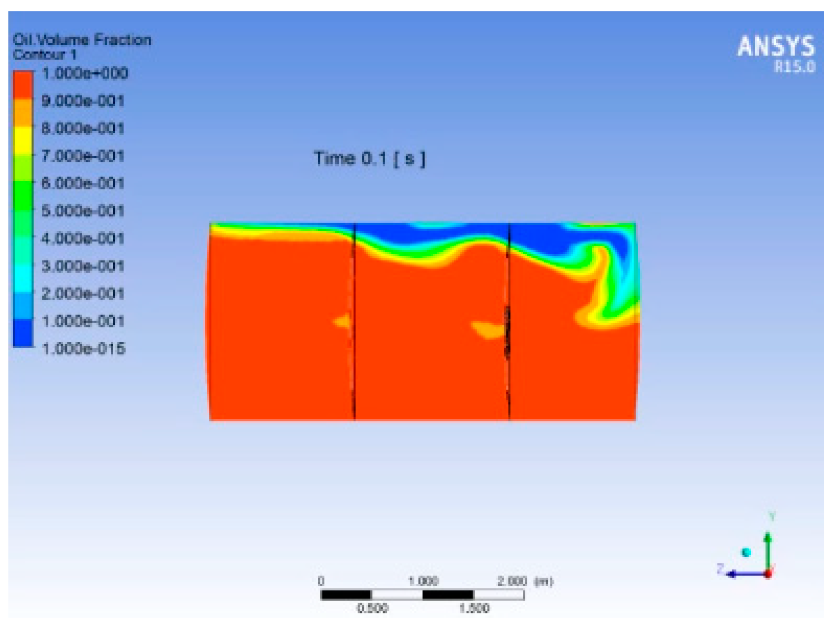
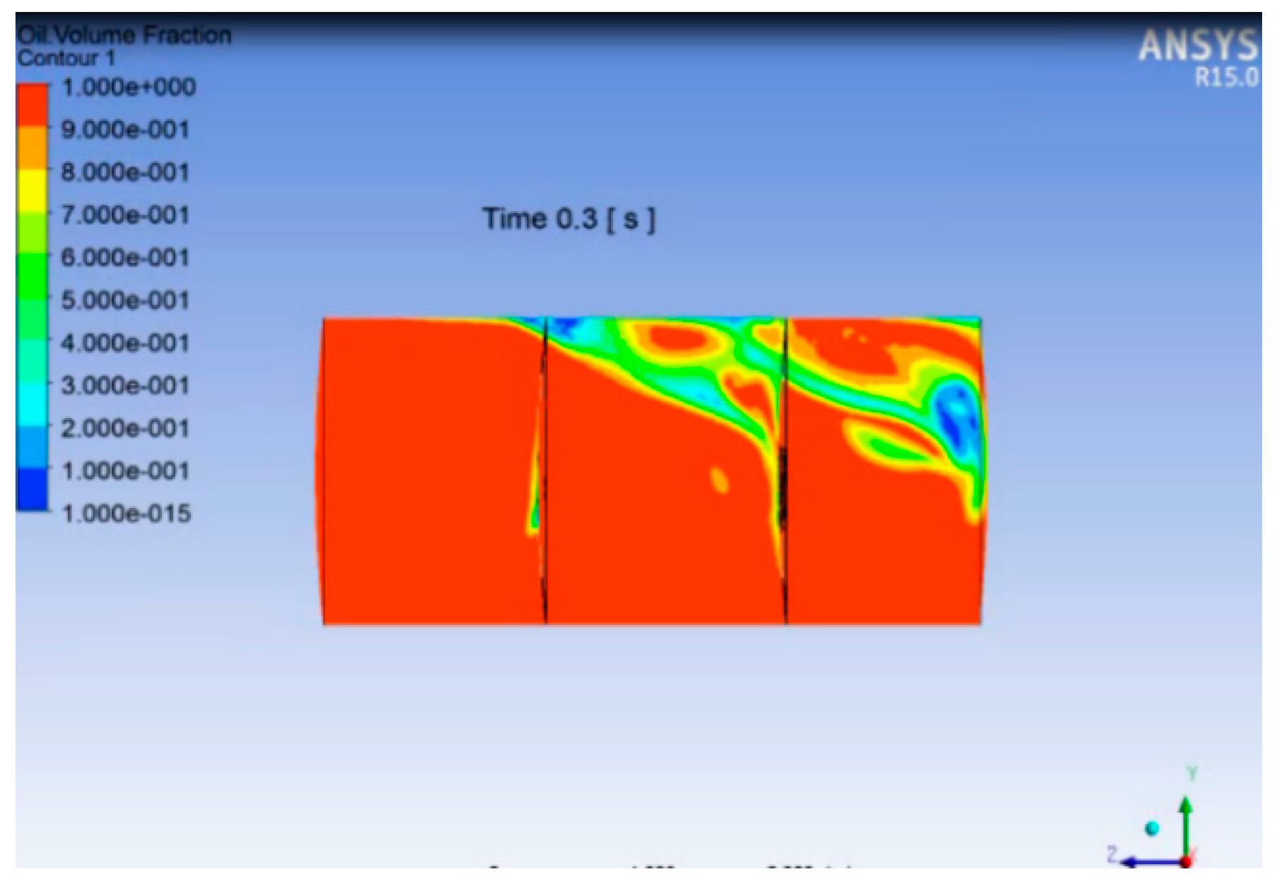
Case 4: Abnormal Deceleration
The slosh results i.e., the pressures generated with respect to time at all three monitor points for Case 4 are shown in 
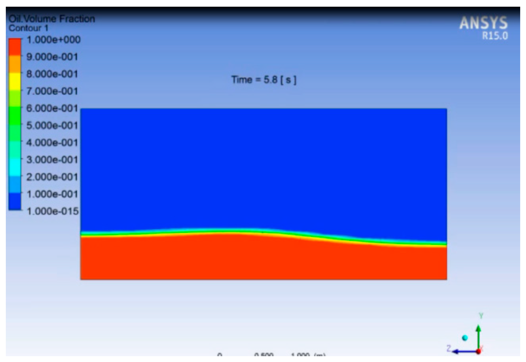
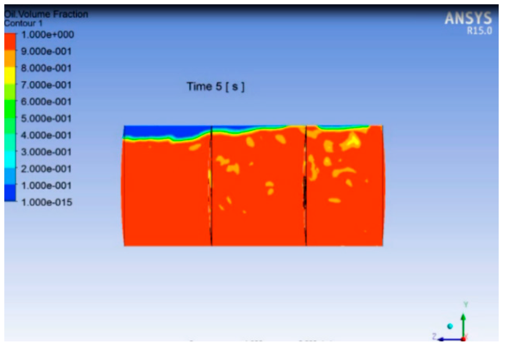
Figure 24. Similar to case 3, opening pressures were exceeded for the first 0.2 s at point 2 and point 3. However, the pressures reached in Case 4 were slightly higher than Case 3 due to the abnormal case. Also, an air pocket was found beneath the valve when the valve opened i.e., for the first 0.2 s (Appendix A, Figure A35). This confirms that the air/vapor mixture leaked out during that interval.
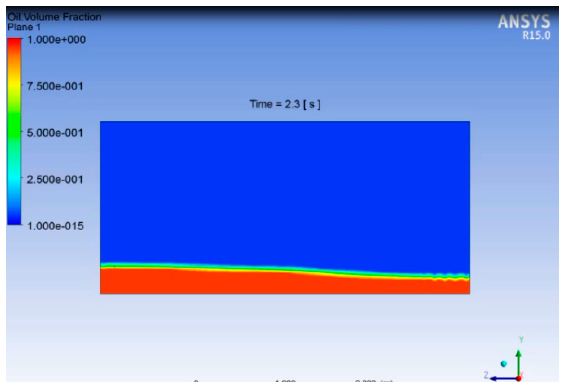
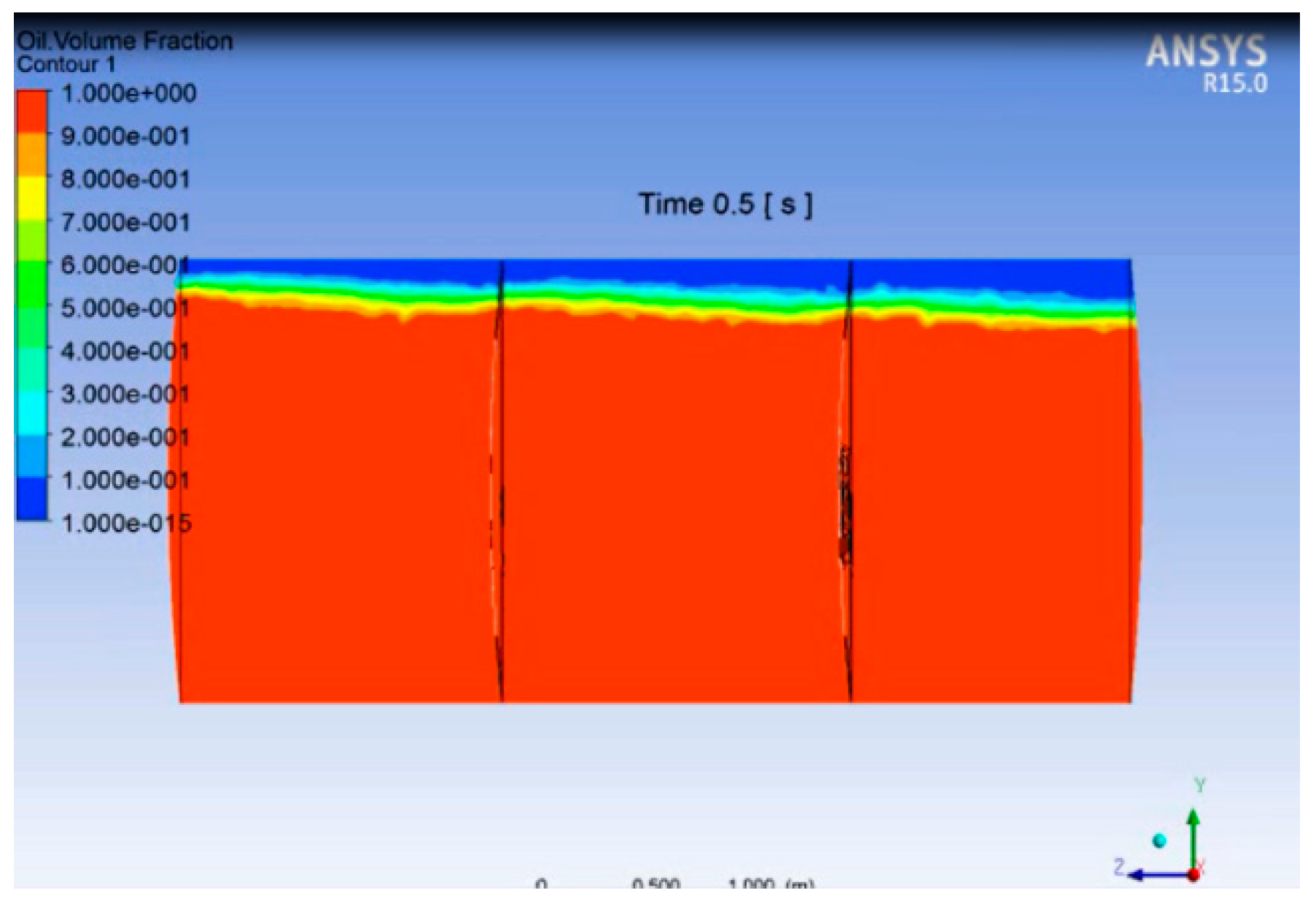
The slosh results showed that the valve of the last compartment did not open even in abnormal cases of acceleration and deceleration. However, the valve of the first and second compartments did open in both cases of deceleration. However, the duration in which the valve opened was less than 0.2 s. Screenshots from the simulation can be seen in Appendix A.
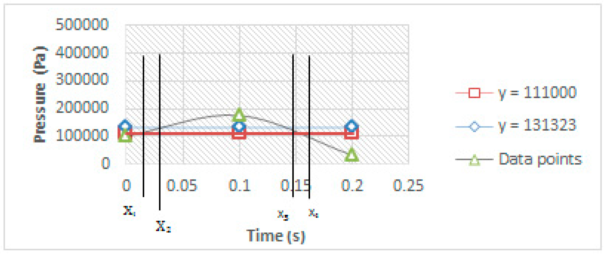
The pressure obtained from sloshing in the normal and abnormal cases of deceleration in compartment 1 and 2 exceeded the cracking pressure of the valve. At 0.1 s, the pressure was much higher than the cracking pressure. At 0.2 s, the pressure dropped down below atmospheric pressure. It rose to atmospheric pressure at 0.4 s and remained nearly at atmospheric pressure for the rest of the simulation time. Hence, to find the loss from the valve in the first 0.2 s, three data points were selected. One was atmospheric pressure at 0 s. The second and third were the pressures obtained from sloshing at 0.1 s and 0.2 s respectively. A curve fit was made to fit all three data points (Figure 25). Two more lines were plotted:
Y = 111,000
Y = 131,323
Both these lines intersect the curve at two points. Hence, all four points were found using simultaneous equations. To do so, the quadratic equation was set equal to 111,000 and 131,323. x1 and x4 were obtained by finding the roots of the equation when the right-hand side of the equation was set equal to 111,000. Similarly, x2 and x3 were obtained by finding the roots of the equation when the right-hand side of the equation was set equal to 131,323. The quadratic equations and its roots for points 2 and 3 in the deceleration cases are summarized in Table 8.
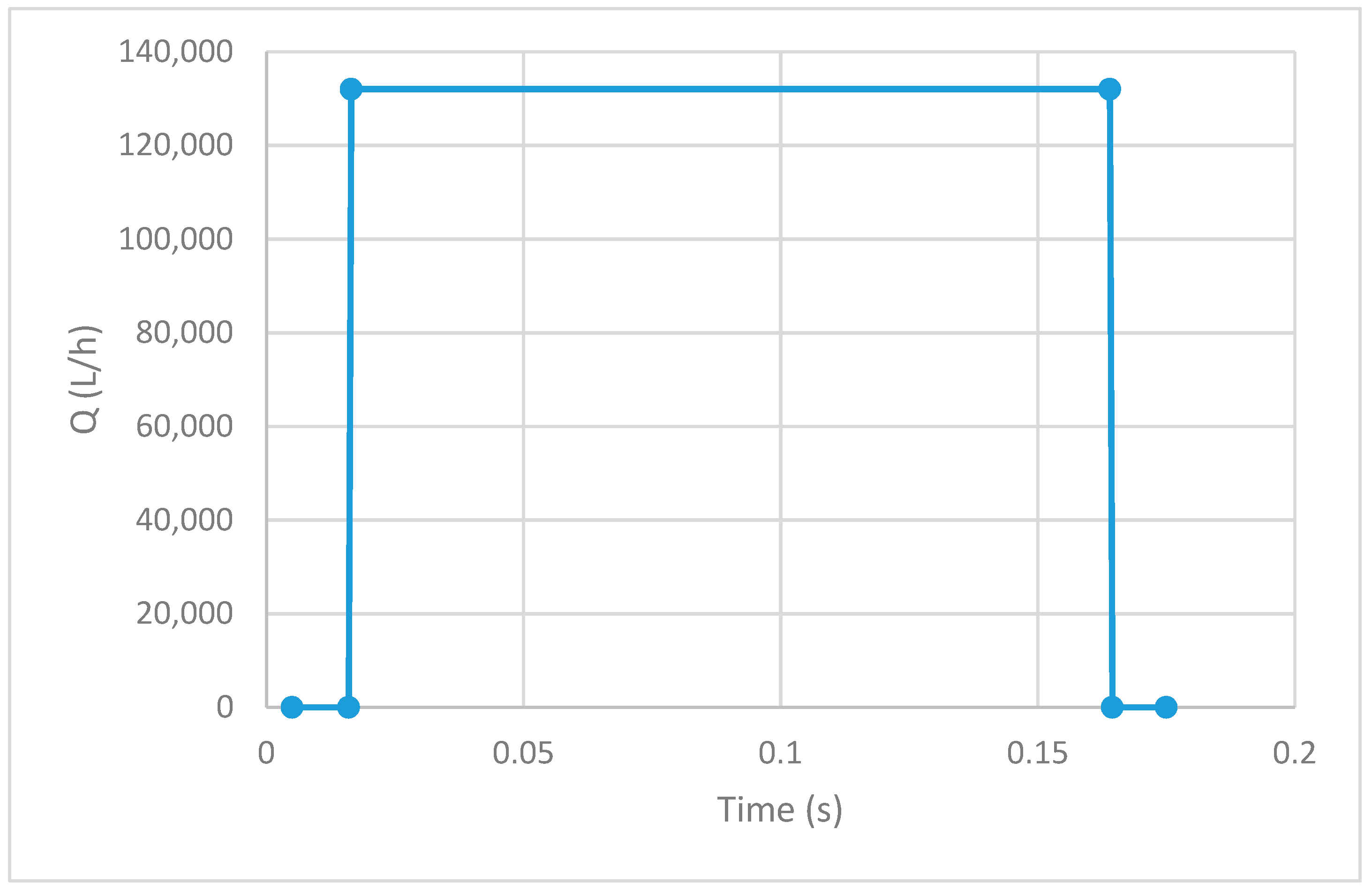
Figure 26 summarizes the flow rate in one case of deceleration between 0.1 s and 0.2 s. From x1 to x2, and from x3 to x4 the flow rate was found using the following equation of region 2:
Q = 6.18025E-47e0.0009*P
This was because x1 intersected the curve at the point where the valve opened i.e., at 111,323 Pa. x2 intersected the curve at the point where the valve was fully open i.e. when the pressure reached 131,323 Pa. x3 intersected the curve at the point where the pressure came back to 131,323 Pa. x4 intersected the curve at the point where the pressure dropped back to 111,323 Pa.
From x2 to x3, the flow rate was found using the following value of the flow rate i.e., region 3:
Q = 132000
As shown in Figure 26, the loss from x1 (0.0053 s) to x2 (0.018 s) and from x3 (0.152 s) to x4 (0.165 s) was calculated using the equation of the flow rate of region 2. Additionally, from x2 (0.018 s) to x3 (0.152 s) was calculated using the equation of the flow rate of region 3.
The loss obtained from all cases is summarized in Table 9 below. A maximum of 0.009 L occurred in a normal case of deceleration per application of brakes from compartment 1 and a maximum of 0.0088 L occurred in a normal case of deceleration per application of brakes from compartment 2. Hence, if the tanker is assumed to brake 500 times over the whole trip, then, a loss of 9 L is obtained due to slosh.
A maximum of 0.01 L also occurred in the abnormal case of deceleration per application of brakes from compartment 1 and a maximum of 0.0096 L occurred in the abnormal case of deceleration per application of brakes from compartment 2. Hence, if the tanker is assumed to brake 500 times over the whole trip, then, a loss of 10 L is obtained due to slosh.
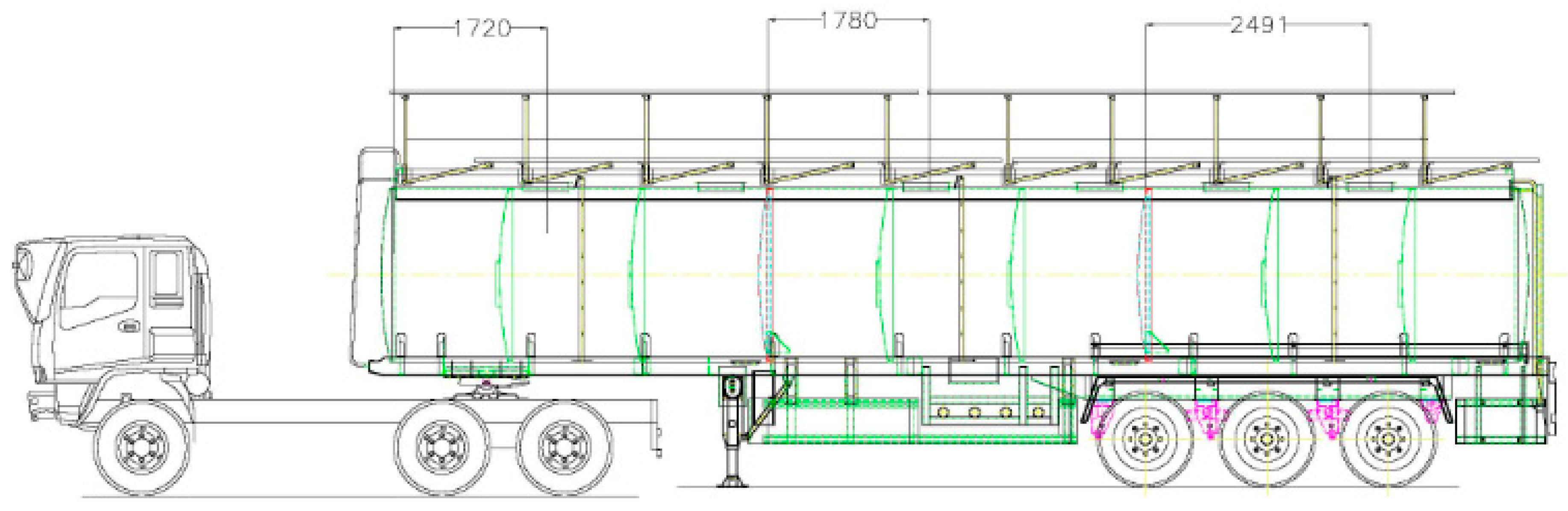
As shown in 
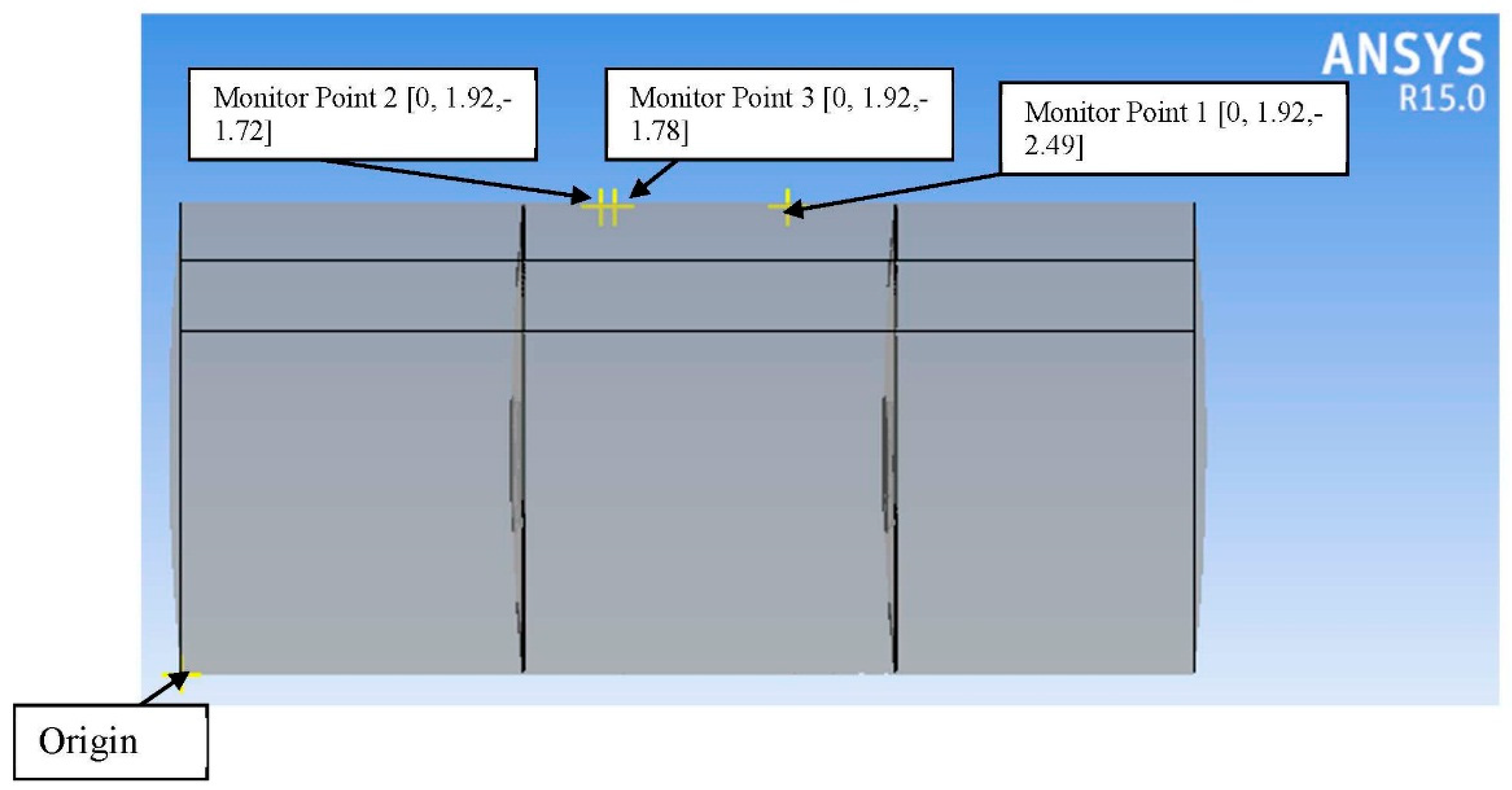
Table 9, no loss was obtained from compartment 3 even in cases of deceleration because of the location of the P/V vent valve. The reason was that the valve was located farthest from the front of the compartment i.e., 2491 mm from the start of compartment 3.
The valves of the first and second compartments were placed at a distance of 1720 mm and 1780 mm respectively from the start of the compartment. Hence, moving the valve slightly along the longitudinal axis may change the loss results drastically.

4. Conclusions

The slosh model was validated by performing various checks on a rectangular tank. All of them were found to be closely comparable with the theoretical values. After validation, slosh simulation was performed on the actual tank. A few acceleration and deceleration functions were given as inputs to the solver. These cases were constructed after reviewing the literature and actual truck driving data. The pressures were then used to calculate the vapor loss due to slosh. The valve location was found to be of considerable importance as pressures vary largely by moving the valve slightly along the longitudinal axis. No loss was found in the third compartment even in abnormal cases of acceleration and deceleration. The location of the valve of the third compartment was farthest from the front of the compartment i.e., 2491 mm from the front of the compartment.
The slosh was not found to contribute much in terms of vapor loss. However, a negligible amount of fuel is lost to the environment in deceleration cases from the first and second compartments. Hence, valve location serves as an important factor in vapor loss. Even if the tanker is assumed to brake 500 times, the tanker still only loses a total of 9 L, and if the tanker brakes 500 times abnormally, it still loses only a total of 10 L over the whole trip.

Author Contributions

Conceptualization, T.A.H.R., and G.H.; methodology and formal analysis, H.M.; software, validation, and resources, M.A. and M.H.A. All authors have read and agreed to the published version of the manuscript.

Funding

This research was funded by Deanship of Scientific Research, King Saud University, through research group number RG-1439-027.

Acknowledgments

The authors are thankful to SZABIST, PNEC-NUST, and GIK Institute for providing necessary technical assistance and resources. The authors also extend their appreciation to the Deanship of Scientific Research at King Saud University for funding this work through research group number RG-1439-027.

Conflicts of Interest

The authors declare no conflict of interest.

Appendix A

Appendix A.1. Slosh Calculation Validation

Figure A1. Free Surface at t = 4.8 s; height = 0.5 m.
Energies 13 02625 g0a1
Figure A2. Free Surface at t = 5.8 s; height = 0.5 m.
Energies 13 02625 g0a2
Figure A3. Free Surface at t = 2.3 s; height = 0.25 m.
Energies 13 02625 g0a3
Figure A4. Free Surface at t = 7.1 s; height = 0.25 m.
Energies 13 02625 g0a4

Appendix A.2. Sensitivity Analysis

Appendix A.2.1. Spatial Coordinates

Mesh = 0.1 m;
Figure A5. Free Surface at t = 0.5 s with a mesh size of 0.1 m.
Energies 13 02625 g0a5
Figure A6. Free Surface at t = 1 s with a mesh size of 0.1 m.
Energies 13 02625 g0a6
Mesh = 0.05 m:
Figure A7. Free Surface at t = 0.5 s with a mesh size of 0.05 m.
Energies 13 02625 g0a7
Figure A8. Free Surface at t = 1 s with a mesh size of 0.05 m.
Energies 13 02625 g0a8
Mesh = 0.04 m;
Figure A9. Free Surface at t = 0.5 s with a mesh size of 0.04 m.
Energies 13 02625 g0a9
Figure A10. Free Surface at t = 1 s with a mesh size of 0.04 m.
Energies 13 02625 g0a10
Mesh = 0.03 m;
Figure A11. Free Surface at t = 0.5 s with a mesh size of 0.03 m.
Energies 13 02625 g0a11
Figure A12. Free Surface at t = 1 s with a mesh size of 0.03 m.
Energies 13 02625 g0a12
Mesh = 0.035 m;
Figure A13. Free Surface at t = 0.5 s with a mesh size of 0.035 m.
Energies 13 02625 g0a13
Figure A14. Free Surface at t = 1 s with a mesh size of 0.035 m.
Energies 13 02625 g0a14

Appendix A.2.2. Temporal Coordinates

t = 0.1 s;
Figure A15. Free Surface at t = 0.5 s with a step size of 0.1 s.
Energies 13 02625 g0a15
Figure A16. Free Surface at t = 1 s with a step size of 0.1 s.
Energies 13 02625 g0a16
t = 0.2 s;
Figure A17. Free Surface at t = 0.6 s with a step size of 0.2 s.
Energies 13 02625 g0a17
Figure A18. Free Surface at t = 1 s with a step size of 0.2 s.
Energies 13 02625 g0a18
t = 0.25 s;
Figure A19. Free Surface at t = 0.5 s with a step size of 0.25 s.
Energies 13 02625 g0a19
Figure A20. Free Surface at t = 1 s with a step size of 0.25 s.
Energies 13 02625 g0a20
t = 0.05 s;
Figure A21. Free Surface at t = 0.5 s with a step size of 0.05 s.
Energies 13 02625 g0a21
Figure A22. Free Surface at t = 1 s with a step size of 0.05 s.
Energies 13 02625 g0a22

Appendix A.3. Slosh Simulation Result

Case 1:
Figure A23. Free Surface at t = 0.3 s (Case 1).
Energies 13 02625 g0a23
Figure A24. Free Surface at t = 0.5 s (Case 1).
Energies 13 02625 g0a24
Figure A25. Free Surface at t = 4.4 s (Case 1).
Energies 13 02625 g0a25
Figure A26. Free Surface at t = 5 s (Case 1).
Energies 13 02625 g0a26
Case 2:
Figure A27. Free Surface at t = 0.1 s (Case 2).
Energies 13 02625 g0a27
Figure A28. Free Surface at t = 0.5 s (Case 2).
Energies 13 02625 g0a28
Figure A29. Free Surface at t = 4.2 s (Case 2).
Energies 13 02625 g0a29
Figure A30. Free Surface at t = 5 s (Case 2).
Energies 13 02625 g0a30
Case 3:
Figure A31. Free Surface at t = 0.1 s (Case 3).
Energies 13 02625 g0a31
Figure A32. Free Surface at t = 0.6 s (Case 3).
Energies 13 02625 g0a32
Figure A33. Free Surface at t = 1.8 s (Case 3).
Energies 13 02625 g0a33
Figure A34. Free Surface at t = 4 s (Case 3).
Energies 13 02625 g0a34
Case 4:
Figure A35. Free Surface at t = 0.1 s (Case 4).
Energies 13 02625 g0a35
Figure A36. Free Surface at t = 0.3 s (Case 4).
Energies 13 02625 g0a36
Figure A37. Free Surface at t = 0.5 s (Case 4).
Energies 13 02625 g0a37
Figure A38. Free Surface at t = 4.2 s (Case 4).
Energies 13 02625 g0a38
Figure A39. Free Surface at t = 5 s (Case 4).
Energies 13 02625 g0a39

References

  1. Alessandro Vincenzo, D. Modeling of Tank Vehicle Dynamics by Fluid Sloshing Coupled Simulation. Ph.D. Thesis, Mechanical Engineering, Department of Mechanical Engineering, Politecnico Di Milano, Milan, Italy, 2011. [Google Scholar]
  2. Shadloo, M.S.; Oger, G.; Le Touze, D. Smoothed Particle Hydrodynamics Method for Fluid Flows, Towards Industrial Applications: Motivations, Current state, and Challenges, Computers & Fluids. Comput. Fluids 2016, 136, 11–34. [Google Scholar]
  3. Hosain, M.L.; Rönnberg, K.; Bel Fdhila, R. Air flow inside rotating electrical machines: A comparison between finite volume and SPH method. In Proceedings of the Conference Proceedings of NAFEMS World Congress 2017 (NWC17), Stockholm, Sweden, 11–14 June 2017. [Google Scholar]
  4. Goodarzi, M.; Safaei, M.R.; Karimipour, A.; Hooman, K.; Dahari, M.; Kazi, S.N.; Sadheginezhad, E. Comparison of the Finite Volume and Lattice Boltzmann Methods for solving natural convection heat transfer problems inside cavities and enclosures. Abstr. Appl. Sci. 2014, 2014, 762184. [Google Scholar] [CrossRef]
  5. Sadeghi, R.; Shadloo, M.S.; Hirschler, M.H.; Hadjadj, A.; Nieken, U. Three-dimensional lattice Boltzmann simulations of high density ratio two-phase flows in porous media, Computers & Mathematics with Applications. Comput. Math. Appl. 2018, 75, 2445–2465. [Google Scholar]
  6. Kuzniatsova, M.; Shimanovsky, A. Definition of Rational Form of Lateral Perforated Baffle for Road Tanks. Procedia Eng. 2016, 134, 72–79. [Google Scholar] [CrossRef] [Green Version]
  7. Brar, G.S.; Singh, S. An Experimental and CFD Analysis of Sloshing in a Tanker. In Proceedings of the 2nd International Conference on Innovations in Automation and Mechatronics Engineering, ICIAME 2014, Gujarat, India, 7–8 March 2014. [Google Scholar]
  8. Aditya, J.Y.; Akash, B.; Dibakar, R. Effect of baffles on sloshing impact pressure of a baffles tank. In Proceedings of the 11th International Symposium on Plasticity and Impact Mechanics, Implast 2016, New Delhi, India, 11–14 December 2016. [Google Scholar]
  9. Martin, M.; Milan, Z.; Peter, P. Dynamic analysis of fuel tank. In Proceedings of the 20th International Conference: Machine Modeling and Simulations, MMS 2015, Terchová, Slovakia, 7–9 September 2015. [Google Scholar]
  10. Sudheer, S.; Ashok, S. Liquid sloshing in a moving tank—CFD. In Proceedings of the 6th International and 43rdNational Conference on Fluid Mechanics and Fluid Power, MNNITA, Allahabad, India, 15–17 December 2016. [Google Scholar]
  11. United Nations Economic Commission for Europe. European Agreement Concerning the International Carriage of Dangerous Goods by Road; United Nations Economic Commission for Europe: Geneva, Switzerland, 2014. [Google Scholar]
  12. Government of Pakistan. Oil and Gas Regulatory Authority; S.R.O.900 (I)/2009; Government of Pakistan: Islamabad, Pakistan, 2009.
  13. European Standard. EN 14595—Tanks for the Transport of Dangerous Goods—Service Equipment—Breather Device; European Standard: Brussels, Belgium, 2005. [Google Scholar]
  14. Bureau Veritas. TUV NUMBER TȔ. AGG 414-07—ART. 41.63.50—European Standards Certifications AFNOR Norms; Bureau Veritas: Paris, France, 2009. [Google Scholar]
  15. Normec. 41.63.50—Pressure and Vacuum Internal EN Breather Vent; Normec: Castagnito, Italy, 2017. [Google Scholar]
  16. ANSYS CFX Tutorials, v12.0.1 and v13.0; ANSYS Inc.: Canonsburg, PA, USA, 2013.
  17. Cangel, Y.A. and Boles, M.A. Thermodynamics: An Engineering Approach, 7th ed.; McGraw Hill: New York, NY, USA, 2010. [Google Scholar]
  18. Automobile Corporation of Pakistan. 48000 Liter, 3C Tank Design—Shell Pakistan; Automobile Corporation of Pakistan: Sindh, Pakistan, 2019. [Google Scholar]
  19. Verizon Telematics Technical Information Bulletin. In Hard Brake and Hard Acceleration; Verizon Telematics: Georgia, GA, USA, 2019.
  20. James, M.W.R.B.E.; Christopher, W.B. A Computer Based Mathematical Model for Predicting the Braking Performance of Trucks and Tractor-Trailers; Highway Safety Research Institute, University of Michigan: Ann Arbor, MI, USA, 1972. [Google Scholar]
  21. Dodge, F.T. The New Dynamic Behavior of Liquids in Moving Containers; SouthWest Research Institute: San Antonio, TX, USA, 2000. [Google Scholar]
  22. Rao, S.S. Mechanical Vibrations, 4th ed.; Pearson: London, UK, 2004. [Google Scholar]
Figure 1. Valve manufacturer specification [15].
Energies 13 02625 g001
Figure 2. Flow rate model of the valve.
Energies 13 02625 g002
Figure 3. Input acceleration pulse.
Energies 13 02625 g003
Figure 4. Valve location in all compartments [18].
Energies 13 02625 g004
Figure 5. Monitor locations.
Energies 13 02625 g005
Figure 6. Velocity function (Case 1).
Energies 13 02625 g006
Figure 7. Acceleration function (Case 1).
Energies 13 02625 g007
Figure 8. Velocity function (Case 2).
Energies 13 02625 g008
Figure 9. Acceleration function (Case 2).
Energies 13 02625 g009
Figure 10. Velocity function (Case 3).
Energies 13 02625 g010
Figure 11. Deceleration function (Case 3).
Energies 13 02625 g011
Figure 12. Velocity function (Case 4).
Energies 13 02625 g012
Figure 13. Deceleration function (Case 4).
Energies 13 02625 g013
Figure 14. Input acceleration pulse (Slosh Validation).
Energies 13 02625 g014
Figure 15. Mode 1 wave shape.
Energies 13 02625 g015
Figure 16. Periods from the pressure data.
Energies 13 02625 g016
Figure 17. Periods from the maximum free surface height data.
Energies 13 02625 g017
Figure 18. Periods from the minimum free surface height data.
Energies 13 02625 g018
Figure 19. Slosh sensitivity analysis (spatial).
Energies 13 02625 g019
Figure 20. Slosh sensitivity analysis (temporal).
Energies 13 02625 g020
Figure 21. Pressure (Case 1).
Energies 13 02625 g021
Figure 22. Pressure (Case 2).
Energies 13 02625 g022
Figure 23. Pressure (Case 3).
Energies 13 02625 g023
Figure 24. Pressure (Case 4).
Energies 13 02625 g024
Figure 25. Curve fit between data points to determine vapor loss.
Energies 13 02625 g025
Figure 26. Flow rate of the valve vs. time for the curve fit.
Energies 13 02625 g026
Table 1. Valve data points provided by the manufacturer.
Pressure (Pa)Flow Rate (L/h)
120,0005
131,323132,000
Table 2. Valve Model.
RegionPressure (Pa)Flow Rate (Q) (L/h)Cracking Pressure (Pa)
1101,323–111,0000111,000
2111,000–131,322 6.18025 × 10 47 e 0.0009 P
3131,323 and above132,000
Table 3. Mesh Detail.
Curvature Normal Angle (Default)45 degree
Minimum Face Size0.029 m
Maximum Face Size0.03 m
Maximum Size0.03 m
Minimum Edge Length (Default) 1.1475 × 10 4 m
Growth rate (Default)1.85
Table 6. Sensitivity Analysis (Spatial).
Maximum Element Size (m)Number of ElementsMaximum Generated Pressure (Pa)
0.1823,300 1.0142 × 10 5  
0.051,645,183 1.0137 × 10 5  
0.042,608,066 1.0136 × 10 5  
0.0353,613,626 1.0136 × 10 5  
0.035,507,684 1.0136 × 10 5  
Table 7. Sensitivity analysis (temporal).
Time Step (s)Maximum Generated Pressure at Monitor Point (Pa)
0.05 1.014 × 10 5  
0.1 1.0136 × 10 5  
0.2 1.0133 × 10 5  
0.25 1.0132 × 10 5  
Table 8. Roots of the quadratic equation in deceleration cases to determine vapor loss.
CaseMonitor PointQuadratic Equationx1x2x3x4
3Point 2P = −10899999t2 + 1835000t + 1013230.00530.0180.1520.165
3Point 3P = −10899999t2 + 1835000t + 1013230.00540.0180.150.163
4Point 2P = −10999999t2 + 1989900t + 1013230.0050.0160.1640.175
4Point 3P = −10999999t2 + 1989900t + 1013230.00510.0170.160.172
Table 9. Vapor loss due to sloshing.
CaseCompartment 1Compartment 2Compartment 3
Maximum Pressure Compartment 1 (Pa)Fuel Lost (Liter) per Application of Brake/AccelerationMaximum Pressure Compartment 2 (Pa)Fuel Lost (Liter) per Application of Brake/AccelerationMaximum Pressure Compartment 3 (Pa)Fuel Lost (Liter) per Application of Brake/Acceleration
1 1.01 × 10 5   No loss 1.01 × 10 5   No loss 1.01 × 10 5   No loss
2 1.01 × 10 5   No loss 1.01 × 10 5   No loss 1.01 × 10 5   No loss
3 1.77 × 10 5   0.00903 1.73 × 10 5   0.008896 1.09 × 10 5   No loss
4 1.91 × 10 5   0.009974 1.86 × 10 5   0.009637 1.09 × 10 5   No loss

